Intuitive visualization of surface properties of biomolecules

(1)

Intuitive visualization of surface

properties of biomolecules

Raluca Mihaela Andrei

PhD Thesis in Molecular Biology 2012

Supervisor: Monica Zoppè

(2)

(3)

To my brother,

Ciprian

(4)

(5)

The greater the obstacle,

the more glory in overcoming it.

(6)

(7)

RM Andrei – PhD thesis CONTENTS

LIST OF ABBREVIATIONS

3D – three-dimensional aa – amino acid

APBS – Adaptive Poisson-Boltzmann Solver API – Application Programming Interface ATP – adenosine tri-phosphate

CG – computer graphics CPK – Corey-Pauling-Koltun CPU – central processing unit EP – electrostatic potential GE – game engine

GFP – green fluorescence protein GPU – graphics processing unit GUI – Graphic User Interface MD – Molecular Dynamics

MEL – Maya Embedded Language MLP – molecular lipophilic potential NMA – Normal Mode Analisys OS – oligosaccharide chains RGB – red, green, blue

RMSD – root mean square deviation

(12)

(13)

RM Andrei – PhD thesis ABSTRACT

ABSTRACT

In living cells, proteins are in continuous motion and interaction with the surrounding medium and/or other proteins and ligands. These interactions are mediated by protein features such as Electrostatic Potential (EP) and hydropathy expressed as Molecular Lipophilic Potential (MLP). The availability of protein structures enables the study of their surfaces and surface characteristics, based on atomic contribution. Traditionally, these properties are calculated by phisico-chemical programs and visualized as range of colours that vary according to the tool used and imposes the necessity of a legend to decrypt it. The use of colour to encode both characteristics makes the simultaneous visualization almost impossible. This is why most of the times EP and MLP are presented in two different images. In this thesis, we describe a novel and intuitive code for the simultaneous visualization of these properties.

For our purpose we use Blender, an open-source, free, cross-platform 3D application used for modelling, animation, gaming and rendering. On the basis of Blender, we developed BioBlender, a package dedicated to biological work: elaboration of proteins motion with the simultaneous visualization of their chemical and physical features.

Blender's Game Engine, equipped with specific physico-chemical rules is used to elaborate the motion of proteins, interpolating between different conformations (NMR collections or different X-rays of the same protein). We obtain a physically plausible sequence of intermediate conformations which are the basis for the subsequent visual elaboration.

A new visual code is introduced for MLP visualization: a range of optical features that goes from dull-rough surfaces for the most hydrophilic areas to shiny-smooth surfaces for the most lipophilic ones. This kind of representation permits a photorealistic rendering of the smooth spatial distribution of the values of MLP on the surface of the protein.

EP is represented as animated line particles that flow along field lines, from positive to negative, proportional to the total charge of the protein.

Our system permits EP and MLP simultaneous visualization of molecules and, in the case of moving proteins, the continuous perception of these features, calculated for each intermediate conformation. Moreover, this representation contributes to gain insight into the molecules function by drawing viewer's attention to the most active regions of the protein.

(14)

(15)

RM Andrei – PhD thesis INTRODUCTION

INTRODUCTION

1 General aspects of visualization

1.1 Visual perception

We are used to perceive information from the surrounding world through the five senses: sight, hearing, smell, touch and taste. The information we receive by sight, apparently without any effort, is the result of an elaboration process involving the eyes and the brain.

Visual perception is the sense which allows the brain to intercept and interpret visible light, creating the ability to see. Amongst the senses, Plato [Plato] considers sight the most noble; while in the other senses, the process implies two parts (a sensor and the sensed, like an ear and a sound), the sight involves three parts – the viewer, the seen and the light. “Of all the senses, trust only the

sense of sight”, said Aristotle [Aristotle], ranking sight the first of the five senses.

The primacy of the visual is emphasized also by the popular phrase “seeing is

believing”.

Several different processes are involved in visual perception. Physiological processes are the reactions of the cones and rods cells to different light waves, which convert photons into a signal that is delivered to the brain throughout the optic nerve. Neuro-psychological processes allow the brain to interpret the stimuli received.

Seeing can be described as the process of decoding the information

1 Figure 1. Examples of incomplete drawings. Our brain is capable to process the information received from eyes and fill the gaps so that we can recognize a triangle with a sphere on each tip, an S shape, a spiky sphere, a snake and a panda. This technique is also used for logos, for example IBM and CNR-IFC.

(16)

present in the acquired image. The Gestalt school of psychology [Koffka1935] believed that our perception is the result of the relation between stimuli, rather than the sum of the existing stimuli. Humans are able to form a complete mental image from incomplete drawings because our brains fill the gaps (Figure 1); thus, vision is not necessarily what we see but how our brain interprets the world around us. Therefore, it is through our own experiences that we shape how we perceive this world.

The fact that we humans are very good at extracting information through visual observation is well synthesized in the old adage “a picture is worth a

thousand words”. Psychological studies showed that humans process visual

information very effectively.

Visual perception is a complex process that cannot be treated in details here. As a short summary it includes [Sutaria1984]:

– colour perception and colour constancy – the ability to distinguish

different colours and to recognise different shades of colour in different light intensities;

– shape perception and shape constancy – the ability to distinguish

shapes and to recognise a shape regardless of size, colour or the angle from which it is viewed;

– spatial relations – interpreting the position of one object relative to

others;

– visual analysis and synthesis – the ability to differentiate between

parts and the whole object (e.g. letters that make up words);

– visual closure – the ability to complete an incomplete image (see

Figure 1);

– visual conceptualizing – the ability to make pictures in mind based

on observations, experiences and data;

– visual discrimination – the ability to interpret differences between

objects observed (e.g. b versus d);

– visual figure-ground distinction – the ability to focus on important

characteristics amidst many (e.g. selecting a blue pencil among many or focusing on a particular word among others);

– visual memory – the ability to store and recall information perceived

with the eyes (e.g. remembering where an object is situated);

(17)

pattern;

– visual sequence – interpreting images in a realistic order (e.g.

arranging pictures of events in the sequence in which they are presented).

1.2 Visualization

Visualization is the process of creating graphical representations such as diagrams, images, animations, maps, etc. from data. It reflects also creative ways of representing data visually. Even excluding highly codified visual elements (letters, words, numbers), there is no limit to what kind of information can be translated into an image.

Visualization is a human activity that arose thousands of years ago with cave paintings, in the attempt of people to transmit their ideas to the others. Since childhood, we use several types of graphical representations to describe things. At kinder garden we draw houses, animals, trees, flowers, people and we discover that images are a good way to communicate what we see. Then, at school, teachers use drawings, schemes, maps to help us understand more quickly concepts from physics, biology, chemistry, history etc.. We all normally draw an approximate map to show someone the indications to a specific location in town. All these are forms of visualization.

1.2.1 Symbols

Symbols surround us in our everyday life, from street signs to computer icons and marks in scientific disciplines (Figure 2). They are an important issue in our lives and are introduced to ease the communication of concepts and the description of phenomena. We all agree on their significance and use them to indicate precise things. Symbols are good instruments for communication, convey unequivocal concepts and they do not raise doubts when seen.

(18)

1.3 Scientific visualization

In 1987, a special issue of Computer Graphics on 'Visualization in Scientific Computing' published the formal definition of scientific visualization [McCormick1987]: “Visualization is a method of computing. It transforms the

symbolic into the geometric, enabling researchers to observe their simulations and computations. Visualization offers a method for seeing the unseen. It enriches the process of scientific discovery and fosters profound and unexpected insights”. The primary goals of Scientific Visualization is to provide insight into

scientific data and to allow scientists an easier way to improve and strengthen their understanding and share their data. The transformation of numerical data into a visual representation organizes them in a way that permits the brain to understand relationships within large amount of data.

The type of data usually visualized are numbers, abstract theoretical quantities or relationships, or reflect a gradation or a change in some quantity with respect to others. These datasets are often converted into contours and isosurfaces, glyphs, colour maps and image information. The main task of these figures is to convey as much information as possible about the dataset when they are observed by viewers, facilitating the recognition of patterns and/or the detection of exceptions.

Visualization represents a way to explore (to search for new things), to analyse (to verify existing hypotheses) and to present (to communicate results). Maybe the most important characteristic of visualization is its ability to go beyond the visual.

Traditional areas of Scientific Visualization are: engineering, medical imaging, biology, chemistry, physics, astrophysics, meteorology etc..

The necessity of computer-aided scientific visualization emerged as a Figure 2. Examples of symbols. Some symbols are commonly used, others are discipline-specific (mathematics-physics, music).

(19)

result of rapid advances in computing and electrical engineering technologies, especially high-performance computing during the mid-1980's. Since that time, scientists and engineers have been flooded with increasing amount of data from experimental equipments and computer simulators.

Complementary to the traditional hypothesis-test method of inquiry, data visualization brings together data from different fields, allowing understanding and processing of enormous amount of information quickly, as it is all represented in a simple image or animation. In this way new questions may arise and more discoveries can be made.

In the last years, the interest in biological processes visualization and divulgation increased enormously. David Goodsell, in the preface of “The machinery of life” wrote that his illustrations are meant to “allow us to look at the molecular structure of cells, if not directly, then in an artistic rendition”. In his books, the molecular drawings are in scale, which permits a comparison of various illustrations to understand the dimensions [Goodsell1998]. Recently, Nature Methods [Nature Methods2010] and Science Magazine [Science2011] dedicated special issues to visualization of biological data. Computer-based visualization is widely used in biology to help understand and communicate data, to generate ideas and to gain insight into biological processes especially with the advent of 'omics' studies. These journal issues present a collection of reviews that examine the methods used to visualize genomes, alignments and phylogenetics, macromolecular structures, system biology data and image-based data.

The huge amount of programs available is an indication that biologists still find that their exact requirements are not met by current tools and often prefer to create their own.

Part of the job of being a scientist is to explain the work to others; these might be colleagues, a wider scientific community or the general public. When a scientist is writing for other scientists he or she typically uses very specific scientific terminology, but when they explain complex cellular mechanisms to the general public they need to use metaphors related to human experience to better engage the imagination, and therefore the perception of the audience.

A more direct and very effective way to explain things is by drawing models. Beyond this basic means of visualizing an idea or an observation, 3D physical or virtual models are nowadays the most significant communication

(20)

method in Molecular Biology. The development of Computer Graphics made explanations of molecular processes even easier by means of animations.

1.3.1 Scientific visualization steps

The basic elements of scientific visualization follow a series of procedural steps, whose boundary is not always clear cut, but which can be roughly classified as:

– data acquisition — scientific data are obtained through an iterative

process which consist of observational processes (satellite, medical, microscopy imaging, genomics, proteomics), experiments and simulations;

– data processing — raw data require adequate transformation

processes to organize, extract and enhance information;

– computer graphics — scientific data is converted into a displayable

form through two or three-dimensional geometrical modelling, rendering and animation processes;

– observation and interaction — visible interaction with the data leads

the user to gain better understanding of the information.

Among the four elements described above, the choices pertaining to the modelling and rendering processes may have the most significant impact on how visualized images are perceived by viewers. In particular, good selection of rendering methods and parameters can produce striking photo-realistic images.

Designers of scientific visualization systems have to consider the influence of the human visual system on how such visual appearances are perceived. The selection of appropriate geometries and visual features for rendering holds the key to generating good information visualization. Colours and parameters of rendering and animations are important in effectively conveying information.

2 Proteins

2.1 Protein architecture

Proteins are polymers of long sequences of 20 different amino acids. Each aa consists of a chiral carbon atom (called α carbon) bonded to an amino group (NH3+), a carboxyl group (COO–), a hydrogen atom and a distinctive side chain

(21)

The specific chemical properties of each aa side chain determine the role of the amino acid in protein structure and function. Amino acids can be grouped in four categories according to the properties of the side chains:

– non-polar aa with hydrophobic side chains that tend to be located in

the interior of the protein, where contact with water is minimal;

– polar aa with hydrophilic side chains that tend to be located on the

surface of proteins and form hydrogen bonds with water;

– basic aa with positively charged and hydrophilic side chains located

on the surface of proteins;

– acidic aa with negatively charged and hydrophilic side chains

usually located on the outside of proteins.

Amino acids are chained together by peptide bond between the carboxyl group of one aa and the amino group of the successive one (Figure 4). They form polypeptide chains of variable length, up to thousands of aa, with two distinct ends: N terminus (the one terminating in an amino group) and C terminus (the one terminating in an carboxyl group).

Figure 4. Polypeptide chain structure. Proteins are formed by a sequence of aa connected by the planar peptide bond (represented here as a rigid plane). The bond length and the direction of rotation of the bonds (ϕ and ѱ rotational angles) are depicted.

Figure 3. Amino acid general structure. The structure of an aa consists of a fixed structure (the same for all aa) formed of an alpha carbon, an amino group, a carboxyl group, a hydrogen, and a variable side chain (residue).

(22)

Four distinct aspects define protein's structure (Figure 5) as described by K.U. Linderstrøm-Lang in 1952 [Linderstrøm-Lang1952]:

– primary structure is the sequence of aa in the polypeptide

[Sanger1951, Sanger1953], also called chain, from N terminus to C terminus;

– secondary structure is the local, regular arrangement of aa in the

polypeptide, stabilized by hydrogen bonds between CO and NH groups of the main chain; the most common are the α-helix and the β-sheet [Pauling1951a, Pauling1951b, Pauling1951c]. An α-helix is a coiled conformation with the CO group of one aa forming a hydrogen bond with the NH group of the aa located four residues downstream along the linear polypeptide chain. A β-sheet is formed by two or more segments of the polypeptide chain (that can be also distant in sequence) lying side by side and held together by hydrogen bonds. It can be composed of several strands, oriented either parallel or antiparallel to each other;

– tertiary structure represents the three-dimensional folding of the

polypeptide chain held by interactions between side chains from different regions of the primary structure [Kendrew1958]. Usually, α -helices and β-sheets are connected by loops and fold into compact globular structures called domains, with hydrophobic aa localized in the interior and hydrophilic aa facing the surface of the protein. The tertiary structure is also determined by the interactions between polar and charged aa side chains, forming hydrogen and ionic bonds. The structure of the proteins in the secretory pathway are further stabilized by S-S bonds between cysteines;

(23)

– quaternary structure consists of interactions between different polypeptides in proteins composed of more than one chain [Svedberg1927].

Additional levels of structural classification can be identified:

– super-secondary structures – proteins show patterns of interaction

between helices and sheets close together in the linear sequence, including α-helix hairpin, β-hairpin and β-α-β unit;

– domains – many proteins contain compact, independent units, called

domains. They are difficult to define precisely and at present the subdivision of structures into domains varies according to the classification used, which can be structural or functional;

Figure 5. Aspects of protein structures.

Primary structure is the sequence of aa. In blue

are coloured the aa that form an α-helix and a

β-sheet (secondary structure). Tertiary

structure represents the 3D organization of the

protein in space. The blue elements of secondary structure show that distant aa in the linear sequence may reside close in the 3D space. Quaternary structure defines the assembly of different polypeptides in multi-chains proteins, in red one domain.

(24)

– modular proteins – they are multi-domain proteins which often contain many copies of closely related domains: for example, fibronectin contains 29 domains including multiple repeats of 3 types of domains called F1, F2 and F3.

Analysis of the structures of proteins revealed similarities between proteins, an important issue of structural biology. A classification of proteins structures can be consulted on SCOP (Structural Classifications of Proteins) [Murzin1995] and CATH (Class, Architecture, Topology, Homologous superfamily) [Orengo1997] databases. Although based on different criteria, these two databases classify proteins structures into 4 categories: all-α (structures essentially formed by α-helices), all-β (structures essentially formed by β-sheets),

α/β (structures with α-helices and β-strands) and α+β (structures in which α -helices and β-strands are largely segregated).

2.2 Why it is important to see proteins

Proteins are essential components of cells and are involved in every aspect of biological activity. They have structural functions (actin, tubulin), mechanical function (myosin), act as transporters of small molecules (myoglobin, haemoglobin) or cellular vesicles (kinesin, dynein), transmit information within (kinases) and between cells (protein hormones), provide defence against infections (antibodies), act as enzymes, receptors, are involved in cell adhesion, cell cycle, DNA transcription and replication, RNA synthesis and the production of more proteins.

Molecular genetics research revealed that many diseases stem from specific protein defects [Alberts1998, Eisenberg2000]. Vast research activity is devoted to protein structures and functions, such as in the field of molecular biology or drug design. Seeing the proteins at work is crucial to understand their behaviour, the mechanisms they are involved in, to be able to create drugs and interfere where necessary. By being able to visualize proteins and other macromolecules in the cellular environment, we could get essential insights in the mechanisms of life.

To accomplish this, an important aspect is the information of the three-dimensional structure of proteins which allows understanding of protein fold and provides an insight into the way the proteins act in vivo. Understanding how particular amino acids residues are involved in protein function, especially when

(25)

combined with knowledge of the 3D structure of proteins, helps to grasp how particular sequences in proteins are involved in biological functions.

2.3 Historical overview of protein visualization

The solution of the 3D structure of myoglobin in 1958 by Kendrew [Kendrew1958] marked the beginning of the new era of structural biology. Since then, a wealth of protein structures has been solved by X-ray crystallography, NMR spectroscopy and cryo-electron microscopy and today the Protein Data Bank (PDB) [Berman2000, Protein Data Bank] counts over 67.000 proteins structures. These data provide much detailed information that help biochemists understand macromolecular functions. Protein structures are obtained and stored as atomic coordinates, which are impossible to interpret by the human brain, therefore they must be presented visually. After solving a protein's structure, its visual representation became the second preoccupation of scientists. Some representation methods are described below.

2.3.1 Physical representations

In 1958, the group of John Kendrew solved the myoglobin three-dimensional structure at 6 Å resolution [Kendrew1958]. Myoglobin is a heme-iron containing protein that carries and stores oxygen in muscle cells. Two years later the same laboratory obtained a map of the protein at 2 Å resolution [Kendrew1960]. For solving the structure of a protein, Kendrew was awarded the Nobel Prize for chemistry in 1962. The first model of a protein was a plasticine model of myoglobin (known also as the 'sausage model') made by Kendrew at Cavendish laboratory in Cambridge (UK). Its cylindrical shape, showing the track of the main chain and supported by wooden rods protruding from a pegboard base can be admired at the Science Museum in London (Figure 6).

(26)

2.3.1.1 All atoms representation Kendrew model

In 1969, Kendrew built the first atomic model of a protein (Figure 7 left); the structure, 1.8 x 2.5 m, looked like a 'forest of rods'.

For the interpretation of the 2 Å map of myoglobin with 1260 atoms (hydrogens excluded), Kendrew invented a new modelling technique inspired from the toy construction kit Meccano. About 2500 steel rods, 1.8 m high, were positioned on the pegboard; these were decorated with coloured clips to indicate the electron density, so that atoms could be positioned. After the insertion of atoms of the main chain, the densities related to the side chains could be seen at appropriate intervals. The scale of the model was chosen 5 cm/1 Å to allow human hand to reach and fix the clips. The positions of the atoms were continually adjusted as the structure was refined.

Figure 6. Myoglobin first physical model. The plasticine model of the main chain of myoglobin, made by Kendrew, is supported on wooden rods.

(27)

Most of the objects, that can be now admired at the Science Museum in London, originally were part of the laboratory where they were handled, discussed, measured, tested against data and corrected and refined.

A similar procedure was employed for the double-helical model of DNA, built of brass models and specially-cut metal bases (Figure 7 right) created by James Watson and Francis Crick from the same Cambridge laboratory.

The Richards Box (Fred's Folly)

In 1968, in a sabbatical year in David Phillips’s lab for structural biology at Oxford University, just after solving the structure of ribonuclease at Yale University, Fred Richards and co-workers introduced an optical comparator [Richards1968] that facilitated the building of Kendrew-style brass models (Figure 8). Electron densities resulting from crystallographic solutions were printed by computers on paper, and electron density contour lines were traced by connecting numbers of similar values on the paper. These contour lines were then traced onto transparent plates (1 x 1 m). The plates were mounted vertically, equally spaced, creating a sliced three-dimensional electron density map. Half-silvered (semi-transparent) mirrors were arranged between the map and the hand-made wire model to superimpose the electron density map upon the brass model and adjust the brass atomic pieces so that they fit the density. As larger molecules were solved, the scale was reduced from 5 cm/Å as used initially to 2.5 cm/Å, and then to 1.0 cm/Å.

The Richard's box remained an indispensable tool used by crystallography labs around the world for about 10 years, when it was finally replaced by Figure 7. First brass models. (left) Kendrew building the all-atom brass representation of myoglobin. The rods help building and stabilizing the complex brass model. (right) The brass model of DNA created by Watson and Crick.

(28)

computer graphics systems. The earliest computer systems were referred to as "electronic Richard's Boxes" and nowadays programs still use the same basic superposition of electron density maps and atomic models for structure building.

2.3.1.2 Backbone trace models

The physical models containing all atoms were large and cumbersome. Backbone trace models were used to simplify the polypeptide chain as a series of virtual bonds connecting the α−carbons. The protein fold is specified by the bend angles for each α−carbon and the torsion angles along virtual bonds. Two examples of this category were in use in the 1970's: Byron Rubin's wire-bender model and Blackwell Molecular Models.

Byron Rubin's wire-bender model

The wire-bender model consists in a 3 mm-diameter steel rod bent according to the pattern of α-carbon chain of a protein. The bending was accomplished by means of a machine (Byron's Bender [Rubin1972, Rubin1985]) Figure 8. Richard's Box device. Behind the half-silvered mirror at the top is a transparent plastic sheet with a trace of a section of the electron density map. Gazing directly into the mirror, one can see the electron density superimposed with the physical model (at bottom). Light boxes at the bottom sides illuminate the section of the physical model represented according to the electron density map. Multiple plastic sheets containing different sections of the electron density map are stored in a rack at the top right (out of view).

(29)

and a list of torsion and bend angles. The shortcoming is variability of the scale, since the α−carbon to α−carbon length is not fixed. For the first time, Byron Rubin introduces the ribbon representation of proteins: helices for α-helices and arrows for β-strands, a very common representation of proteins structures in nowadays software. The small backbone wire models from Byron's Bender were the most manipulable and portable models available at the time (Figure 9).

An example illustrating the importance of models occurred at a scientific meeting in the mid 1970's. David Davies brought a Bender model of an immunoglobulin Fab fragment, and Jane and David Richardson brought a Bender model of superoxide dismutase [Beem1977]. While comparing these physical models at the meeting, they realized that both proteins use a similar fold, despite having only about 9% sequence identity. This incident was the first recognition of the occurrence of what is now recognized as the immunoglobulin superfamily domain in unrelated proteins. The insight was published in a paper entitled "Similarity of three-dimensional structure between the immunoglobulin

domain and the copper, zinc superoxide dismutase subunit" [Richardson1976]. Blackwell molecular models

Blackwell Molecular Models [Fletterick1982, Fletterick1985] (Figure 10) are more complicated and provide more chemical information. It is a ball-and-stick model system representing α−carbon positions and the peptide link between adjacent alpha carbons.

Figure 9. Byron Rubin brass ribbon models. (left) rubredoxin and (right) human neutrophil collagenase (on permanent exhibition at the Smithsonian Institution, Washington DC USA, 28 cm)

(30)

They are made of plastic, in twenty different colours to code for amino acid type, which push-fit together at 1 cm/Å scale and the α-carbon to α-carbon bond length is 3.8 cm. The scales and indices observed on the balls and rods serve to mark the angle of bend and the angle of torsion of consecutive amino acids in the molecule. This system allows the attachment of specific side chains. Support rods are added after the model is built, to fix some of the distances between α -carbons and to stabilize the finished model.

Since then, various groups built protein models, a significant collection can be seen at http://3dmoleculardesigns.com/.

Figure 10. Blackwell representation. The 9 aa of an α −helix are identified by letters from a to i. Each element from the kit is identified by a number, to ease building of macromolecules. The spheres and rods are provided with verniers and scales to set atomic diameters and the bend, torsion and dihedral angles.

(31)

2.3.2 Computer representations

Physical and CG representations co-evolved in the early times of structural biology, both used to understand protein structure.

1960's – 1970's

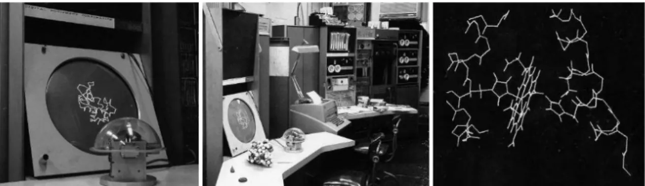
In 1966, Cyrus Levinthal and his colleagues at Massachusetts Institute of Technology developed the first system [Levinthal1966] to display what we call today a “wireframe” representation of molecules structures on a monochrome oscilloscope screen (the terminal display was named Kludge, and it was developed at Project MAC (Mathematics and Computation) [Stotz1963]), shown in Figure 11.

The three-dimensional effect was achieved by rotating constantly the structure on the screen. The rate of rotation was controlled by a globe-shaped device on which the user rested his/her hand (an ancestor of today's trackball). At that time, the full potential of such a set-up was not completely settled. The conclusion of Cyrus Levinthal's description of the system in Scientific American, indicated that there was no doubt that it was paving the way for the future: “It is

too early to evaluate the usefulness of the man-computer combination in solving real problems of molecular biology. It does seems likely, however, that only with this combination can the investigator use his 'chemical insight' in an effective way. We already know that we can use the computer to build and display models of large molecules and that this procedure can be very useful in helping us to understand how such molecules function. But it may still be a few years before we have learned just how useful it is for the investigator to be able to interact

Figure 11. First device for wireframe representation. (left) The screen with the globe that control the direction and speed of image rotation. (middle) Overview of the molecular modelling system, with the Kludge in the lower left corner. Notice the space-filling models in front of the screen. (right) Details of the structure of myoglobin, showing the heme group with two segments of the polypeptide chain surrounding it.

(32)

with the computer while the molecular model is being constructed.”

Levinthal's forecast slowly developed in the following decades. In 1965, Carroll K. Johnson, from Oak Ridge National Laboratory, released ORTEP (Oak Ridge Thermal-Ellipsoid Plot Program) [Johnson1965], a program written in FORTRAN, to produce stereoscopic drawings of molecular and crystal structures with a pen-plotter (Figure 12). The stereoscopic view aid the visualization of complex macromolecules. It rapidly became a favourite tool of crystallographers to produce illustrations of structures for conference presentations and publications. This program is still in use, and its latest version, ORTEP III, was released in 2000. The current version retains all features and functionality of the original, with the exception of the output which is now displayed on the screen, instead of being printed on paper.

These programs could not directly interpret the crystallographic data; the electron density maps were converted into Kendrew “sticks” models and the coordinates, measured by hand were introduced into the computer to build the virtual model. The next important step molecular visualization was the development of software tools able to interpret crystallographic data.

In the mid 1970's, superoxide dismutase [Beem1977] was the first protein solved crystallographically and visualized entirely with computers by David and Jane Richardson and colleagues. They used a density-fitting computer system called "GRIP" at the University of North Carolina [Tainer1982].

In the late 1970's, more and more crystallographers made the transition to building models for newly solved protein crystals with computers ("electronic Richards' boxes") rather than with physical Kendrew-style models. One of the major advantages was that the computer kept track of the atomic coordinates, Figure 12. ORTEP system. (left) ORTEP pen-plotter machine. The physical model of the same molecule drawn also by ORTEP can be seen in the image. (right) Example of stereoscopic drawing designed with ORTEP.

(33)

contrary to the Kendrew model where atomic coordinates had to be measured manually, atom by atom. Four systems were widely used: (1) MMS-X, developed at the Computer Systems Laboratory at Washington Univesity in St. Louis [Barry1974, Miller1981], (2) GRIP-75 at the Computer Science Department of the University of North Carolina at Chapel Hill [Tsernoglou1977, Brooks1977, Wright1981, Lipscomb1981, Pique1991], (3) BILDER developed at the Medical Research Council Laboratory for Molecular Biology in Cambridge, England [Diamond1981a, Diamond1981b], and (4) FRODO [Jones1978, Jones1981, Jones1985].

1980's

In 1980, TAMS (Teaching Aids for Macromolecular Structure) project [Feldmann1980] produced the first stereo views of macromolecules (Human Immunoglobulin G). The stereo projection was obtained by using two conventional slide projectors equipped with orthogonal polarizing filters, each viewer wearing polarized glasses. This technique is still in use today and to make easier the understanding of the three-dimensionality of the molecules on printed documents, the images are displayed side-by-side (Figure 13).

During the 1980's, the most popular computer system for crystallographers was manufactured by Evans & Sutherland. These computers displayed the electron density map and enabled an amino acid sequence to be fitted manually into the map. The colour display showed a wireframe rendering of the amino acid chain, and could be rotated in real time. These systems used scalable vector graphics. Rapid rotation was accomplished with three hardware Figure 13. Stereo slide pair from the TAMS project. The example shown here is a crossed eyes stereo of human IgG 'DOB', alpha carbons only; carbohydrate white, light chain yellow, heavy chains red and blue.

(34)

matrix multipliers (one for each dimension, X, Y, and Z). The software package most often used on E&S computers was FRODO (now evolved to Turbo-FRODO).

During the 1980's, David and Jane Richardson pioneered computer graphics representations of molecular structure with a series of programs developed at Duke University. In the late 1980's, this led to a program called CHAOS written in Evans and Sutherland PS300 function-net language [Richardson1989].

In 1981 Fermi and Perutz published the 'Atlas of Molecular Structures' with stereodiagrams of myoglobin and haemoglobin. To facilitate the viewing, the diagrams were printed in red and green and a foldable pair of red-green glasses was delivered with the book. This technique to provide images with stereoscopic 3D effect is called anaglyph.

The anaglyph images consist of two colour layers (red and green or cyan) superimposed with an offset with respect to each other and the 3D effect is perceived by wearing glasses with coloured lens: red for the left eye and green or cyan for the right eye.

1990's

With the gradual progress of Computer Graphics tools and techniques, the development of software for protein visualization increased. For example, Molscript program [Kraulis1991], by Per Kraulis and released in 1991, was the successor of ORTEP, developed in 1965. Molscript is one of the main programs currently used for plotting protein structures.

A team led by TA Jones, from Uppsala, Sweden wrote the program O [Jones1991], in 1991. The program is designed for scientists with a need to model, build and display macromolecules. O is mainly aimed at the field of protein crystallography, bringing into use several tools, which ease the building of models into electron density, allowing this to be done faster and more correctly.

In 1992, the Richardsons described the kinemage (from kinetic image), interactive animated images of molecules, and their supporting programs MAGE and PREKIN [Richardson1992]. By virtue of its implementation on the Macintosh, this was the first program which brought molecular visualization to a large number of scientists, educators, and students. The programs were described in the lead article in the first issue of the journal Protein Science (early 1992), and the program itself was provided on a diskette which accompanied that issue. This

(35)

article also included instructions for using the program PREKIN together with MAGE for authoring new kinemages. In the subsequent five years, over a thousand kinemages accompanied articles in Protein Science, the majority being authored or edited by Jane Richardson.

Software tools for general use

The first tools for visualization of macromolecular structures were used only by specialists. The increasing number of macromolecular structures solved contributed to the development of software tools for general use, easier to handle.

In 1992, Roger Sayle developed RasMol (Raster – the array of pixels on a computer screen – Molecules), an open-source, command-line and stand-alone program for macromolecular visualization [Sayle1992, Sayle1995]. The software included a ray-tracing algorithm that could shade solid objects as they rotated in space. The users explore the molecules structures via a scripting language which permits selection of proteins chains, different colouring and representations. RasMol is one of the most successful software due to an excellent compromise between rendering speed and image quality which permits even large molecules to be rotated in real-time. RasMol was the first program to run on personal computers. Before it, visualization software ran on graphics workstations only.

Since then a wealth of visualization tools have been created and now everybody can use them with minimum effort. Tools like Chimera [Pettersen2004, Chimera], MOLMOL [Koradi1996, MOLMOL], PMV [Sanner1999], PyMOL [DeLano, PyMOL software], Swiss-PDBViewer [Guex1997, Swiss-PdbViewer], VMD [Humphrey1996, VMD], Yasara [Krieger2002] are widely used. A full list of free molecular visualization programs can be consulted on The World Index of BioMolecular Visualization Resources web page [MolVisIndex].

Besides these stand-alone tools, web-based plug-ins were developed such as Chime MDL [Chime] and Jmol [Jmol viewer, Jmol website], integrated on Protein Explorer [Martz2002, Protein Explorer] and Proteopedia web-sites [Hodis2008, Proteopedia] respectively, and FirstGlance, PDBe, RSCB PDB.

Additionally to protein structure visualization, these programs provide also other important analysis tools for proteins characterization: alignment, side chains building, energy minimization, calculation of surface properties, such as electrostatic potential and hydropathy.

(36)

Shading Language (included in software such as VMD and PyMOL), which is used to write small programs, called shaders (described below in Rendering section), that produce sophisticated visual effects. QuteMol [Tarini2006] (Figure 14 left) goes a step further and uses GLSL to produce illustrative rendering effects, computing ambient occlusion to better display three-dimensionality of the molecules. ProteinShader [Weber2009] (Figure 14 right) is a Java-OpenGL molecular visualization tool that introduces pen-and-ink style rendering for ribbons to enhance the three-dimensionality and uses shaders to map text labels onto the surfaces of ribbons and tubes, shown in colours.

Animations

Using 2D images to show the structure of biomolecules, large part of the 3D information is lost. If images are worth a thousand of words, then animations are worth much more and scientists became aware of the power of molecular movies to communicate their results. Although animations are costly in terms of user effort and computing time (hundreds or thousands of individual images are needed for a rendered movie) they are useful to highlight important features by offering a 'guided tour' of structures and macromolecules interactions.

In 1978, Harrison's group at Harvard solved the first atomic resolution structure of a spherical virus [Harrison1978]. A movie was the way they chose to divulgate the assembly of the virus; they shot with a 16 mm film with a Bolex camera from a computer screen, frame-by-frame. Thus, the movie showing the virus assembly became self-explanatory.

The remarkable progress in computer power and software tools permitted the development of programs to include movie generation, for example Chimera Figure 14. Examples of protein representations. (left) space-filling representation using QuteMol and (right) ribbon representation using ProteinShader.

(37)

or eMovie [Hodis2007] (a plug-in for PyMOL) enabling scientists to create informative molecular animations about their research. The commands include rotations, zooms, fading, colouring and different representations.

2.4 Experimental visualization techniques

Humans curiosity to understand biology contributed to the development of sophisticated techniques and methods for biological investigation. The easiest way to understand the shape of things is to look at them, with the help of light. Visible light is part of the electromagnetic spectrum (Figure 15), which extends over a wide range of frequencies (or wavelengths) and includes also radiowaves, microwaves, infrared, ultraviolet, X-rays and γ-rays.

When the objects under investigation are too small to be seen by the naked eye, proper instruments are needed. By exploiting different regions of the electromagnetic spectrum and the interaction of atoms with radiation, important information can be acquired about the structure and dynamics of proteins. A wide range of techniques are available for studying proteins.

2.4.1 Microscopy data

The basic technique used by biologists is optical microscopy. With a Figure 15. Electromagnetic spectrum size scale. Electromagnetic spectrum frequencies and wavelengths and a comparison between the wavelength and the size of macro and micro scale objects.

(38)

resolution of 0.2 µm, cells and large subcellular organelles such as nuclei, chloroplasts and mitochondria can be observed. Usually, the cells are fixed in order to stabilize and preserve their structure (brightfield and darkfield microscopy) and then stained with dyes to increase the contrast between the different components (brightfield microscopy).

It is also possible the visualization of living cells, without staining (phase-contrast microscopy) or by labelling the molecules of interest using fluorescent markers (the most used is Green Fluorescent Protein – GFP) to study their intracellular distribution (fluorescence microscopy). A variety of methods have been developed to study the displacement (fluorescence recovery after bleaching – FRAP) and interactions (fluorescence resonance energy transfer – FRET) of GFP-labelled proteins in living cells.

2D images are very informative, but cells are three-dimensional entities. The introduction of laser and various complex arrangements of mirrors contributed to obtain 3D high-resolution images of the samples (confocal, multi-photon excitation, super-resolution fluorescence, stimulated emission depletion – STED, photo-activated localization – PALM, stochastic optical reconstruction microscopy – STORM) [Cooper2007].

To visualize components of the cell smaller than 100 nm, light microscope is not suitable due to its limited resolution. Using electrons with wavelength of 0.004 nm, electron microscopes can achieve a greater resolution than light microscope, down to 1-2 nm. Two distinct phenomena are involved in various EM techniques: electrons transmission (transmission electron microscopy – TEM) through the specimen and electrons scattering (scanning electron microscopy – SEM). The observation of samples in their native environment is possible at cryogenic temperatures (-195 °C) by means of cryo-electron microscopy and cryo-electron tomography, which creates 3D reconstructions from 2D images.

These are the classical microscopy techniques, included in textbooks. The high speed of technical development and newest scientific discoveries contribute to the continuous development of new microscopy techniques. Almost every week, a new and sophisticated technique is published.

2.4.2 Atomic data

To investigate molecular structures at atomic level (Ångström – 10-10_m),

(39)

magnetic resonance (NMR) spectroscopy [Wüthrich1995, Kai1997]. The interpretation of the results obtained by these techniques is not unambiguous and entails assumptions and approximations depending upon knowledge of the protein from other sources, including biochemistry.

X-ray crystallography [Drenth1994] is a technique that exploits the fact

that X-rays are diffracted by the crystals. X-rays (wavelength 0.5-1.5 Å) are scattered by the electron clouds of the atoms of the studied molecule. For good results, high-quality crystals are needed; the best crystals are pure, perfectly symmetrical, containing a vast number of three-dimensional repeating arrays of precisely ordered, identical molecules. The effect of ordering the molecules in crystals is to enhance the intensity of the scattered signal. The crystals are usually very small (< 1 mm) and can be of different shape, from perfect cubes to long needles, obtained by growing concentrated solutions of the molecule in different conditions, such as temperature, pH and concentration of salts and protein. The crystal is rotated while it is bombarded with X-rays, providing electron diffraction maps. From the intensity of each diffraction spot in the 2D maps for different angles, the value of electron density can be calculated in every point of 3D coordinates (xyz), using Fourier transform. Next, all values of electron densities are integrated and 3D maps are obtained. A model is then progressively built into the experimental electron densities, refined against the data until an accurate molecular model is obtained and the position of each atom in the crystal can be retrieved.

Although very important residues have been (and will be) obtained by X-ray crystallography, the technique has some limitations: for example hydrogen position is very difficult to retrieve, since they have only one electron. Some proteins are refractory to crystallization (membrane proteins or very dynamic loops of proteins, considered disordered parts). The accuracy of the structure determination is validated by the resolution, a measure of how much data was collected. More data acquired, more details are present in the electron-density map features. The resolution is expressed in Å, lower value meaning higher resolution. Values lower than 1.5 Å indicate less ambiguity in positioning the atoms. An index of the structural quality is the R-factor, a measure of how well the model reproduces the experimental data. It is expressed as a percentage of disagreement between the observed diffraction pattern and the calculated model. R-factors less than 20% indicate well determined structures.

(40)

Nucleic magnetic resonance spectroscopy [Wüthrich1995, Kai1997] is

a method used to obtain information about the structure and the dynamics of proteins by exploiting the magnetic properties of certain atomic nuclei (2H, 15N or

13_{C). NMR is performed on aqueous samples of highly purified proteins labelled}

with 13C and 15N and introduced in a magnetic field. The results are chemical shift spectra relative to a reference signal. From these chemical shifts, a set of distances between atomic nuclei that define both bonded and non-bonded close contacts in the molecule are retrieved. Using this information, the atoms positions are calculated, usually more conformations being solved, which may reflect structural dynamics. In general, more internuclear distances measured indicate a higher accuracy of the models. NMR spectroscopists report overall RMSD between the atoms in secondary structure elements in all coordinates sets in the ensemble of structures as a measure of structure quality. An RMSD value of 0.7 Å indicates high-quality structures. In contrast to X-ray crystallography, NMR has been limited to relatively small proteins, usually smaller than 35 kDa. New development allows for NMR study of large proteins as shown in reviews [Mittermaier2006, Tzakos2006, Foster2007].

Electron microscopy arose as a technique usually used to solve 3D

structures of large ensembles, such as viruses, nucleic pores, ribosomes; with a few Å resolution, it bridges the gap between the atomic information of single molecules and the micron size information of cellular data (between the molecular and cellular structure) [Studer2008, Zhou2011].

Interdisciplinarity

Biology is a discipline that encompasses many orders of magnitude in size and time. Even considering only the cell level, there is a difference of 6 orders of magnitude between the size of the cell and the dimension of an atom. In order to gain a deep understanding of biology it is necessary to combine data provided by different research fields like biochemistry, genetics, biophysics, molecular and cellular biology, structural biology, immunology, visualization techniques, etc.. Interdisciplinarity is key to build a rich image of cellular environments and processes. Cells are delimited by a lipid bilayer, the plasma membrane. The interior of the cell is a crowded ambient, with the cellular components (nucleus, endoplasmic reticulum, Golgi apparatus, proteins and small molecules) immersed in water solution. Here, the inhabitants are involved in a vast range of

(41)

processes (from responding to outside signals that induce muscle contraction or production of antibodies to synthesis of new proteins or cellular division). All these processes are part of the cellular activity that can be understood only merging knowledge from various research fields.

2.4.3 Databases

Atomic databases

Protein structures are deposited on the Protein Data Bank [Berman2000, Protein Data Bank], a freely accessible repository of experimentally determined three-dimensional structures of macromolecules. The majority, 85%, were solved using X-ray crystallography. These data are stored in .pdb files (identified by a 4-digits number), which contain several information: macromolecule's name and its organism of origin, experimental procedure used to obtain the structure and the detailed parameters, the authors and the related references, the primary and the secondary structure, specification of number of NMR models where the case, various structure refinement methods and their parameters, details about geometry and stereochemistry (covalent bonds length and angles, torsion angles, planar groups, cis-trans geometry etc.), list of heterogeneous atoms in the entry, connectivity between residues and other molecules (oligosaccharide chains, ligands, etc.). The largest part is dedicated to define the position (3D coordinates) of all atoms. Each line includes the atom identity, the corresponding amino acid, the chain identifier, the atomic x, y, z coordinates, occupancy parameters and thermal parameters (also called B-factor, an indication of the relative mobility of an atom). The file can also report the connectivity annotation (covalent bonds, disulfide bonds). The PDB file format can be read by humans. Each line in a .pdb file is self-identifying and consists of 80 columns.

A crystallographic PDB entry stores atomic coordinates of the crystal asymmetric unit (ASU), rather than of the biological assembly (also referred to as the biological unit) which is the functional form of a biomolecule. An ASU may contain one biological assembly, a portion of a biological assembly or multiple biological assemblies. Starting from ASU, several symmetry operations consisting in translations, rotations or their combinations may be needed to obtain the biological assembly. PDB entries contain two records that define the biomolecule: REMARK 300, which provides its subunit composition related to ASU and REMARK 350, which cites the matrices needed to build it from the

(42)

ASU. For example, if a homodimeric protein crystallizes with a monomer in the ASU, REMARK 300 mentions one chain and REMARK 350 two matrices. But if there is a dimer in the ASU, REMARK 300 cites two chains, and REMARK 350, only the identity matrix.

Raw data databases

The Protein Data Bank stores the final results of a molecular structure study: the 3D coordinates of each atom. The raw data, such as NMR spectra and electron microscopy density maps are stored in more specific data bases (NMRShiftDB [NMRShiftDB], nmrdb [nmrdb], EMDataBank [EMDataBank], Electron Microscopy Databank [Electron Microscopy Databank]).

Visualization databases

For human interpretation of structural data, visualization instruments are needed. Proteopedia is a powerful web tool to communicate 3D information about macromolecules structures. It is a wiki system that facilitates sharing among the scientific community and has an additional educational component. Proteopedia contains a page for every entry of Protein Data Bank and the Jmol window incorporated allows the user to explore the structure of interest by rotating, zooming, changing the representation (atoms, ribbon, surface) and colouring it (by atom, by amino acid, by secondary structure) etc..

Also the Protein Data Bank and its mirrors offer means of visualization and other ways to explore structural data.

2.5 Protein structure and properties representation

Despite the fact that pdb files are human readable, atomic coordinates sets are impossible to interpret by humans, therefore protein structures are presented visually. Several standard representations exist for proteins:

balls-and-sticks for atoms and bonds, to visualize covalent bonds, space-filling diagram

with the atoms visualized as spheres with van der Waals radii to visualize the space occupied, ribbons as helices or tubes for α-helices and strands or arrows for β-strands to capture the protein secondary structure and surfaces to visualize the interaction with the medium: solvent accessible surface (Lee-Richards [Lee1971]) and solvent-excluded surface (Connolly [Connolly1983]). The information about the atom identity is often delivered by a standard colour-code introduced by Corey, Pauling and Koltun in 1953 (known also as the CPK model):

(43)

red for oxygen, blue for nitrogen, grey for carbon, white for hydrogen, etc. [Corey1953, Koltun1965]. Not all visualization tools respect this code, adopting new ones (e.g. PyMOL uses green for carbon). When studying proteins, scientists choose the most appropriate of these representations to visualize their protein according to the interest of their study. When standard codes are used, it becomes easy to communicate biological information through images, transmitting to the viewers the author's message.

2.5.1 Protein surfaces

In structural biology, the surface of a protein can be defined in three ways: van der Waals, solvent accessible and solvent excluded (molecular), as shown in Figure 16.

The van der Waals surface, also called space-filling molecular model is obtained by the union of all atoms drawn as rigid spheres with van der Waals radii. It approximates the space occupied by the macromolecule.

The solvent accessible surface is the part of a molecule exposed to the solvent, is calculated by the rolling-ball algorithm (usually the water molecule with the radius of 1.4 Å) and is traced by the centre of the sphere as it rolls over the van der Waals surface.

The molecular surface is considered as a bulk in the solvent and it is Figure 16. Surface calculation. Three surfaces are commonly used: Van der Waals, solvent accessible and solvent excluded (Connolly).

(44)

traced by the contact points of the sphere rolling over the van der Waals surface. The rolling-ball algorithm was developed by Frederic Richards and independently implemented three-dimensionally by Michael Connolly in 1983 [Connolly1983] and Tim Richmond in 1984 [Richmond1984].

Several programs are available to calculate the solvent excluded surface, including MSMS (Michel Sanner's Molecular Surface or Maximal Speed Molecular Surface) [Sanner1996], NACCESS [NACCESS], Surface Racer [Tsodikov2002], ASC [Eisenhaber1993, Eisenhaber1995] and Molecular Surface Package [Connolly1993].

Since the surface of a protein is determined by the position of its atoms at any given moment, atomic motion implies that the surface can change in time. This concept applies both to the fast vibrational movements (bond vibrations, rotameric flipping and rotation of chi angles in long side chains) and to the slower conformational changes related to protein activities and intrinsic flexibility (such as disordered loops, or domain motion). For this reason, our system is set to calculate the surface of moving proteins on a frame by frame basis, showing in a visual manner the curvature properties of the molecule as they change in time.

Surface curvature is an important feature for the characterization of the shape of proteins and it is at the basis of shape complementarity; more concave surfaces are more favourable to binding of small molecules and ligands. In practice, the application of ambient occlusion during the rendering of images reveals the curvature feature of the surface.

Two surface properties, electrostatic potential and hydropathy, are usually visualized on the molecular surface.

2.5.2 Protein surface properties

In living cells, proteins are in continuous interaction with other macromolecules and the surrounding medium. In these interactions, two volumetric properties, electrostatic potential and hydropathy have a significant role. These physico-chemical properties are deployed locally along the surface, and understanding surface properties is important to understand proteins functions and interactions with other molecules. Protein-protein interactions are mediated by their molecular surfaces and are governed by the properties of the atoms that line the surfaces, such as hydropathy and electrostatic potential.

(45)

2.5.2.1 Hydropathy

Hydropathy is an important physico-chemical property of the protein surface, relevant to its propensity to establish molecular interactions. Hydrophilicity is the propensity of a surface to establish hydrogen bonds with water or polar solvents. On the opposite, hydrophobicity is the propensity to repeal water and preferentially associate with other hydrophobic surfaces. It can be estimated at the various levels: for example, in proteins it is considered that aliphatic and aromatic amino acids are non-polar and hydrophobic; O- and N-containing aa side chains are polar and hydrophilic. Hydropathy is usually expressed as numerical value calculated according to one of several formula, whereas hydrophobicity/hydrophilicity is a more practical measure of how strongly the molecule repeals water.

Walter Kauzmann introduced the term ‘hydrophobic bonding’ to describe interactions driven by exclusion of water [Kauzmann1959]. Hydrophobic interactions are important non-covalent forces that are responsible for different phenomena such as structure stabilization of proteins [Privalov1988, Hendsch1994, Wimley1996, Southall2002], folding of proteins [Dill1990], protein-protein interaction [Mueller2002] and maintenance of the lipid bilayer organization of membranes [Tanford1973]. The importance of hydrophobicity in protein stability, proposed theoretically by Kauzmann, was confirmed by the solution of first protein structure showing that hydrophobic residues are indeed preferentially buried in the protein interior [Kendrew1958].

Calculation of hydrophobicity is important in identifying various protein features such as membrane spanning regions and buried residues, which are highly hydrophobic or antigenic sites, exposed on the surface and which are hydrophilic domains. Usually, these calculations are shown as a plot along the protein sequence, making it easy to identify the location of potential protein features. The hydrophobicity is calculated by sliding a fixed size window (covering an odd number of aa) over the protein sequence. At the central position of the window, the average hydrophobicity of the entire windows is plotted (Figure 17).

(46)

Kyte-Doolittle scale [Kyte1982] is the most widely used for detecting hydrophobic regions in proteins. Additionally, several hydrophobicity scales have been published for various protein studies: Engelman [Engelman1986] for prediction of transmembrane regions, Hopp-Woods [Hopp1983] for identification of potential antigenic sites, Cornette [Cornette1987] for prediction of alpha-helices, Rose [Rose1985] and Janin [Janin1979] for determination of buried amino acid residues of globular proteins. All these scales assign hydrophobicity values to each aa (Figure 18).

The differences between the systems shown above, with respect to the Figure 18. Examples of hydrophobicity scales.

Figure 17. Hydrophobicity/hydrophilicity plot. The plot along the aa sequence, using Kyte-Doolittle scale.