URBAN FLOWS SIMULATOR BASED
ON COMPLEX SYSTEM OF QUEUES:
PROCEDURES FOR SIMULATOR
GENERATION
LEONARDO PASINI
ANDSAMUELE SABBATINI
Department of Computer Science, University of Camerino, Via del Bastione 1, Camerino, Italy
(received: 4 September 2015; revised: 13 November 2015; accepted: 23 November 2015; published online: 2 January 2016)
Abstract: In a previous work [Pasini L and Feliziani S 2013 TASK Quart. 17 (3) 155], we have defined an object library that allows the building of architectural models of urban traffic systems. In this work we illustrate the procedures that enable us to produce a system simulator starting from the architectural model of an urban vehicular traffic system.
Keywords: traffic systems, queuing networks, modeling and simulation
1. Introduction
In the scientific work that we are developing [1–4] we define a system of urban traffic as a system that consists of a street network and traffic flows that pass through it. In this context, the network nodes are represented by road intersections and the edges between the nodes are represented by urban roads. The intersections can be road intersections or roundabouts. In both cases there may be traffic light systems aimed at the regulation of traffic flows. The aim of the study is to understand the behavior of the traffic flow in the network. This study is done by building simulators of the corresponding traffic system. In a previous work [1] we have defined an object library that allows us to model a generic system of urban traffic. In this paper we describe a technique that allows a specific system of urban traffic to be associated to a description file system. We call this the Model.datfile.
The file contains a list of data objects that are contained in the library [1] and that form an architectural model of the traffic system. Given then a system of urban traffic by the procedure that we describe in section 3 of this paper, we can produce a Model.dat file that is associated to the system. The Model.dat
file describes the architectural model of the system which is realized by means of the objects in our library.
In section 4 of this paper we define the BuildMod procedure. This procedure automates the process of creating a traffic system simulator that we want to analyze. In fact, when it is executed, the BuildMod procedure reads the data from the Model.dat file of the system and generates the components of the architectural model of the system running their inter-connection. The product that comes from the execution of the BuildMod procedure is the simulator of the traffic system to be analyzed.
Figure 1. Process model of creation
2. An example of an urban system of vehicular traffic
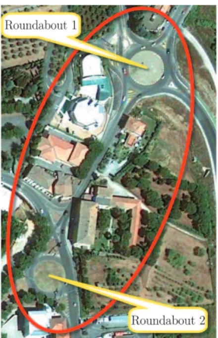
In this paper we consider an example of the urban road network described in Figure 2.This figure is extracted from Google Maps and represents an area north of the city of Siena, which is located in central Italy. This urban road network is shown in Figure 3.
This road system has been described in Section 2 of our previous work [1]. It consists of two roundabouts and two intersections without traffic lights. Figure 3 indicates, with green color, the streets of input to the system from the outside, with red roads outside the system and with yellow roads within the system. Each street is provided with a unique identifier, which is the integer shown in Figure 3. Grade intersections in the road network are identified by integer numbers that are shown in Figure 3. In our previous work [1] we used this system to illustrate the use of the objects of our library in the creation of an architectural model of the system. In this paper we continue the previous study. In Section 3 we describe the procedure to create the Model.dat file that lists the data of the architectural model of the traffic system. In Section 4 we describe the procedure called BuildMod that generates the system simulator based on the information contained in the Model.datfile.
Figure 2. Google maps – image of the Siena Nord system
3. Procedure for generating the Model.dat file
In this section we analyze the first step of the process described above in Figure 1. In the following pages we describe the structure of the Excel file. This file is used for the process of entry of data that characterize the urban traffic system that is the subject of the study.
The file consists of multiple sheets. Each sheet has a specific function for the creation of Model.dat. The Model.dat file is produced by activation of a Macro in this Excel file that allows the data to be transferred in each sheet within the Model.datfile. The file contains the following sheets:
• A sheet called “General data” used to enter the general data of the traffic system;
• A sheet used for the input of data relating to each intersection or roundabout that are present within the system of traffic;
• A sheet called “Traffic flows”. In this sheet surveys carried out by the local authority are inserted;
• A sheet called “Routing Probability” for calculation of the choice of routes to be taken by vehicles.
3.1. “General Data” Sheet
This sheet is used for the high-level definition of the model. This paper describes all the global information of the road system. The paper is divided into several sections for a clearer description of the model. Figure 4 represents the “General Data” sheet used for our study.
Figure 4. Example of “General Data” sheet
The first line of the file contains the following information: • NB_INT is the number of intersections in the system;
• NB_ROAD is the total number of streets;
• NB_MP is the number of crosspoint multiplexers; • NB_FL is the number of flows (traffic sources); • NB_MP_RO is the number of road multiplexers.
This information makes up the first section of the Model.dat file using a macro.
Section 1:
&NB_INT NB_ROAD NB_MP NB_FL NB_MP_RO 4 21 13 7 1;
The file continues to provide data on the streets identified in the traffic system. One record is specified for each road with the following fields that characterize the object ROAD library:
• ID_ROAD is an identification code of a street of the model;
• EXT is a flag that indicates whether the channel goes to the outside (EXT = 1) or whether it is internal (EXT = 0);
• LENG_RO is the length of the route in kilometers;
• R_NB_IN is the number of incoming vehicles detected in the road, if there are no detections the value is 0;
• R_NB_OUT is the number of outcoming vehicles detected in the road, if there are no detections the value is 0;
• INTERSEC is a flag that is set to 1 if the road ends in the crosspoint multiplexer or 0 if it ends in a road multiplexer;
• MP o MP_ROAD is the identifier of the road multiplexer or crosspoint multiplexer where the street ends.
These data is generated by running the macro to the following section in the Model.dat file.
Section 2:
&ID_ROAD EXT LENG_RO R_NB_IN R_NB_OUT INTERSEC MP o MP_ROAD NAME 1 0 0.3 77 0 1 1 " Via_Chiantigiana_Castellina"; 2 1 0.1 0 1 " Via_Aosta"; 3 0 0.3 135 0 1 2 " Via_Aosta"; 4 1 0.1 0 5 " Via_Montecelso"; 5 0 0.3 9 0 1 3 " Via_Montecelso"; 6 0 0.12 0 116 0 1 " Via_Chiantigiana_Stellino"; 7 0 0.15 196 0 1 4 " Via_Chiantigiana_Stellino"; 8 1 0.1 0 131 " Via_Fiume"; 9 0 0.3 55 0 1 5 " Via_Fiume"; 10 1 0.1 0 159 " Via_Chiantigiana_Castellina"; 11 0 0.024 0 0 1 12 " VIA11"; 12 0 0.02 0 0 1 6 " VIA12"; 13 0 0.3 155 0 1 7 " Via_Cassia_Nord"; 14 0 0.018 0 0 1 9 " VIA14"; 15 1 0.1 0 81 " Via_delle_Province"; 16 1 0.1 0 100 " Via_Fiorentina"; 17 0 0.3 103 0 1 10 " Via_delle_Province"; 18 0 0.3 65 0 1 11 " Via_Fiorentina"; 19 0 0.018 0 0 1 8 " VIA19"; 20 0 0.022 0 0 1 13 " VIA20"; 21 1 0.1 0 80 " Via_Cassia_Nord";
The sheet continues with the traffic flow identified. Each stream is added to a record composed by the following fields that characterize the Flow object in the library:
• ID_FLOW is the identifier of the flow in the traffic system;
• TIME_ROU is the interarrival time between two consecutive vehicles; • ID_ROAD is the identifier of the road connected to the flow.
This data is generated by running the macro to the following section in the Model.datfile.
Section 3:
&ID_FLOW TIME_ROU ID_ROAD 1 7.84 1; 2 4.53 3; 3 44.44 5; 4 12.00 9; 5 4.36 13; 6 6.90 17; 7 7.50 18;
The sheet continues with the data relating to the multiplexers that are present within the system of traffic. For each multiplexer one record is inserted with the following fields that characterize the multiplexer object in the library: • ID_MPX is the identifier of the multiplexer object in the model;
• NB_SEC_INP is the number of input sections to a crossing in which the multi-plexer may route vehicles;
• NB_INT is the identifier of the crossing of the input sections;
• Sec_In(n) identifies the nth input section accessible from the multiplexer; • Prob_(n) is the probability with which a vehicle is sent from the multiplexer
to the related input section.
By executing the macro these data generate the following section in the Model.datfile.
Section 4:
&ID_MPX NB_SEC_INP NB_INT Sec_In(n) Prob_(n) 1 1 1 1 1; 2 1 1 2 1; 3 1 1 3 1; 4 1 1 4 1; 5 1 1 5 1; 6 1 2 1 1; 7 1 2 2 1; 8 1 2 3 1; 9 1 3 1 1; 10 1 3 2 1; 11 2 3 3 0.36 4 0.64; 12 1 4 1 1; 13 1 4 2 1;
The last section of the “General data” sheet contains data on road multi-plexers that are present in the system. For each multiplexer of the model a record is specified that contains the following fields which characterize the MP_Road ob-ject in the library:
• ID_MP_ROAD is the identifier the object road multiplexer;
• NB_ROAD_OUT is the number of routes on which the road multiplexer can route traffic that passes through it;
• Road_(n) is the identifier of the nth road in which the multiplexer can send via vehicles;
• Prob_(n) is the probability of routing the vehicle on the nth road.
By executing the macro these data generate the following section in the Model.datfile.
Section 5:
&ID_MP_ROAD NB_ROAD_OUT Road_1 Prob_1 Road_2 Prob_2 1 2 11 0.43 12 0.57;
In addition to the description of the system models this sheet is used for insertion of some global parameters of the system. The following are the available parameters:
• The speed of the vehicles used to calculate travel times;
• The space occupied by the vehicles to calculate the number of vehicles that may contain a street;
• The time that the user wants to consider; • Some routing traffic parameters.
3.2. “Crossroad” Sheets
As previously specified the CreaModeldat.xls file contains a sheet for each crossing or roundabout of the system. In our case the sheets 2, 3, 4, 5 are dedicated to the insertion of crossings 1-2-3-4 in the previously described system. These sheets, using the macro, generate sections 6, 7, 8, 9 of the Model.dat file that are listed later. Figure 5 shows the data related to intersection 2 of the system. For this article we chose this crossroad for a better understanding of the various sections of the sheet.
The first section of the sheet shows the general data of the crossing of the system with reference to the library:
• ID_INT is the identification number of the crossing; • NB_SEM is the number of the traffic lights of the crossing; • NB_SEC_INP is the number of input sections;
• NB_SEC_INTER is the number of internal sections; • NB_SEC_OUT is the number of output sections;
• NB_PATH is the number of possible paths inside the crossing;
• D_SEM is the traffic-light cycle duration (i.e. the duration of the red-green-yellow cycle);
• ROUND this flag is set to 1 if the intersection is a roundabout, otherwise 0. For each internal section of the crossing a record is inserted with the following fields:
Figure 5. Example of sheet describing crossroads 2 shown in Figure 3
• TIME_SERVICE is the time required for a vehicle to the cross section (in seconds); • NB_VEHICLE is the number of vehicles that can simultaneously occupy the section. Its value is equal to 1 for the internal sections of the crossings and may be greater than 1 for the inner sections of the roundabouts.
Afterwards the input sections are listed. For each input section a record is inserted whose fields are the following:
• ID_SEC_INP is the identification number of the input section in the intersection; • NB_PATH is the number of crossing paths which a vehicle can follow;
• TIME_SERVICE is the travel time for a vehicle expressed in seconds (time required to cross the section calculated according to its size);
• SEM_FLAG is a flag that indicates the presence (0) or absence (1) of a traffic light;
• NB_VEHICLE is the number of vehicles that can be located simultaneously within the section.
The sheet continues with the specification of the output sections of the intersection. For each output section a record is shown whose fields are the following:
• ID_SEC_OUT is the identifier of the section in the intersection; • TIME_SERVICE is the time of service;
• LINK_SEC_INT is the identifier of the internal section immediately preceding; • LINK_EXIT_ROAD is the identifier of the street where vehicles are driving.
Afterwards paths are inserted in the sheet that a vehicle can cover within the intersection. For each path a record is shown whose fields are the following: • ID_PATH is the identifier of the pathway;
• L_PATH is the length of the pathway expressed in the crossing section number; • S_(n) is the identifier of the nth internal section of the crossing crossed by the
path;
• P_(n) is the priority level that a vehicle has in the nth section of the route; • INPSEC is the identifier of the input section of the path;
In the last part of the sheet, see example Crossing 2 shown in Figure 5 the data relating to the probability of vehicle routing in the paths of the crossing from each input section are shown. For each input section of this intersection a record whose is shown fields are the following:
• ID_INP is the identifier of each input section of the crossing;
• ID_PATH(n) is the identifier of the nth path that a vehicle can follow entering the section;
• PROB_(n) is the probability that a vehicle follow the nth path entering the section.
Below listed are sections 6, 7, 8, 9 of the Model.dat file relating to intersections in our system. In particular, Figure 5 generates section 7 presented below.
Section 6:
&ID_INT NB_SEM NB_SEC_INP NB_SEC_INTER NB_SEC_OUT NB_PATH D_SEM ROUND
1 0 5 20 5 19 0 1;
&ID_SEC_INTERNAL TIME_SERVICE NB_VEHICLE 1 1 1; 2 3 5; 3 1 1; 4 2.4 4; 5 1 1; 6 2.4 4; 7 1 1; 8 2.4 4; 9 1 1; 10 1.8 3; 11 1 1; 12 2.4 4; 13 1 1; 14 2.4 4; 15 1 1; 16 1.8 3; 17 1 1; 18 2.4 4; 19 1 1; 20 2.4 4;
&ID_SEC_INP NB_PATH TIME_SERVICE SEM_FLAG NB_VEHICLE 1 4 1.2 1 2;
2 3 2.4 1 4; 3 4 1.8 1 3; 4 4 1.8 1 3; 5 4 1.2 1 2;
&ID_SEC_OUT TIME_SERVICE LINK_SEC_INT LINK_EXIT_ROAD 1 1 3 2; 2 1 7 4; 3 1 11 6; 4 1 15 8; 5 1 19 10;
&ID_PATH L_PATH ... S_(n) P_(n) ... INPSEC OUTSEC 1 3 1 5 2 10 3 10 1 1; 2 5 1 5 2 10 4 10 6 10 7 10 1 2; 3 7 1 5 2 10 4 10 6 10 8 10 10 10 11 10 1 3; 4 9 1 5 2 10 4 10 6 10 8 10 10 10 12 10 14 10 15 10 1 4; 5 5 5 5 6 10 8 10 10 10 11 10 2 3; 6 7 5 5 6 10 8 10 10 10 12 10 14 10 15 10 2 4; 7 9 5 5 6 10 8 10 10 10 12 10 14 10 16 10 18 10 19 10 2 5; 8 3 9 5 10 10 11 10 3 3; 9 5 9 5 10 10 12 10 14 10 15 10 3 4; 10 7 9 5 10 10 12 10 14 10 16 10 18 10 19 10 3 5; 11 9 9 5 10 10 12 10 14 10 16 10 18 10 20 10 2 10 3 10 3 1; 12 3 13 5 14 10 15 10 4 4; 13 5 13 5 14 10 16 10 18 10 19 10 4 5; 14 7 13 5 14 10 16 10 18 10 20 10 2 10 3 10 4 1; 15 9 13 5 14 10 16 10 18 10 20 10 2 10 4 10 6 10 7 10 4 2; 16 3 17 5 18 10 19 10 5 5; 17 5 17 5 18 10 20 10 2 10 3 10 5 1; 18 7 17 5 18 10 20 10 2 10 4 10 6 10 7 10 5 2; 19 9 17 5 18 10 20 10 2 10 4 10 6 10 8 10 10 10 11 10 5 3; &ID_INP ... ID_PATH(n) PROB_(n) ...
1 1 0.39 2 1.98 3 45.85 4 51.78; 2 5 28.57 6 32.27 7 39.16; 3 8 28.50 9 32.19 10 39.07 11 0.24; 4 12 44.26 13 53.72 14 0.34 15 1.68; 5 16 56.58 17 0.36 18 1.78 19 41.28; Section 7:
&ID_INT NB_SEM NB_SEC_INP NB_SEC_INTER NB_SEC_OUT NB_PATH D_SEM ROUND
2 0 3 2 2 3 0 0;
&ID_SEC_INTERNAL TIME_SERVICE NB_VEHICLE 1 1 1;
2 1 1;
&ID_SEC_INP NB_PATH TIME_SERVICE SEM_FLAG NB_VEHICLE 1 1 1 1 1;
2 1 1 1 1; 3 1 1 1 1;
&ID_SEC_OUT TIME_SERVICE LINK_SEC_INT LINK_EXIT_ROAD 1 1 1 20;
2 1 2 14;
&ID_PATH L_PATH ... S_(n) P_(n) ... INPSEC OUTSEC 1 2 1 5 2 10 1 2;
2 1 2 5 2 2; 3 1 1 10 3 1;
&ID_INP ... ID_PATH(n) PROB_(n) ... 1 1 1;
2 2 1; 3 3 1; Section 8:
&ID_INT NB_SEM NB_SEC_INP NB_SEC_INTER NB_SEC_OUT NB_PATH
D_SEM ROUND
3 0 4 16 4 9 0 1;
&ID_SEC_INTERNAL TIME_SERVICE NB_VEHICLE 1 1 1; 2 1.2 2; 3 1 1; 4 2.4 4; 5 1 1; 6 1.8 3; 7 0.9 3; 8 0 1; 9 1.2 2; 10 0 1; 11 0 1; 12 4.2 6; 13 2.1 6; 14 0 1; 15 0 1; 16 2.4 4;
&ID_SEC_INP NB_PATH TIME_SERVICE SEM_FLAG NB_VEHICLE 1 3 1.2 1 2;
2 3 2.4 1 4; 3 2 3 1 5; 4 1 3 1 5;
&ID_SEC_OUT TIME_SERVICE LINK_SEC_INT LINK_EXIT_ROAD 1 1 3 15;
2 1 7 16; 3 1 14 19; 4 1 15 7;
1 3 1 5 2 10 3 10 1 1; 2 5 1 5 2 10 4 10 7 10 8 10 1 2; 3 7 1 5 2 10 4 10 6 10 9 10 13 10 15 10 1 4; 4 3 5 5 7 10 8 10 2 2; 5 5 5 5 6 10 9 10 12 10 14 10 2 3; 6 5 5 5 6 10 9 10 13 10 15 10 2 4; 7 3 10 5 12 10 14 10 3 3; 8 5 10 5 12 10 16 10 2 10 3 10 3 1; 9 3 11 5 13 10 15 10 4 4;
&ID_INP ID_PATH1 PROB_1 ID_PATH2 PROB_2 1 1 28.51 2 34.84 3 36.65;
2 4 9.21 5 30.67 6 60.12; 3 7 27.03 8 72.97;
4 9 100; Section 9:
&ID_INT NB_SEM NB_SEC_INP NB_SEC_INTER NB_SEC_OUT NB_PATH D_SEM ROUND
4 0 2 1 1 2 0 0;
&ID_SEC_INTERNAL TIME_SERVICE NB_VEHICLE 1 1 1;
&ID_SEC_INP NB_PATH TIME_SERVICE SEM_FLAG NB_VEHICLE 1 1 1 1 1;
2 1 1 1 1;
&ID_SEC_OUT TIME_SERVICE LINK_SEC_INT LINK_EXIT_ROAD 1 1 1 21;
&ID_PATH L_PATH ... S_(n) P_(n) ... INPSEC OUTSEC 1 1 1 5 1 1;
2 1 1 10 2 1;
&ID_INP ... ID_PATH(n) PROB_(n) ... 1 1 1;
2 2 1;
In the sheets relating to crossings some tools are used that help us in some calculations. The first tool (Figure 6) of the sheet refers to the calculation of the size of the length of the internal sections of the roundabout. To do this, the user enters the data with the general measures of the roundabout in the first line and then specifies the size in the other lines, and the system will calculate the exact length and the resulting travel time.
Figure 7 is the second tool. This tool allows us to calculate the probability of selection paths formed in the “Routing Probability” sheet which will then be read on the left side of the intersection sheet. The example refers to the crossroad 3 of the system, denoted by “Roundabout 2” in Figure 3 and represents, for each input section, the probability that the determined reference path to be followed by the input vehicle.
Figure 6. Tool to calculate section travel times
Figure 7. Selection pathway tool
3.3. “Traffic flows” Sheet
After the list of crossroads we proceed to analyze the sheet called “Traffic flows”. This worksheet is used to enter real data of surveys on traffic flows in order to insert the values measured into the model (Figure 8). Figure 9 shows the estimated arrival rate of vehicles for every single flow into the system. In Figure 9 the arrival rate is denoted by “R”, whereas “I” is the inter-arrival time expressed in seconds.
Figure 9. Flow generation calculation
3.4. “Routing Probability” Sheet
The last sheet to be analyzed “Percentages Routing” (Figure 10) is used to calculate the probability with which the vehicles, entering a roundabout will choose the paths to be carried out. The aim is to compute the probability by which a vehicle entering a roundabout by a given street A will leave the roundabout by a given street B. We suppose that B must be different from A. In this context we use the following formula.
Nvehicle= Nvehicle leaving the roundabout− Nvehicle left in A (1)
Thus, for each of the exits of the roundabout, with the exception of the output relative to the street A that we are considering, we will use the following formula to calculate the probability of selection of the output road B:
P =Nvehicle left from road B Nvehicle
(2)
4. The procedure BuildMod
The BuildMod procedure is responsible for reading the Model.dat file instantiating objects required by the traffic system model. The procedure code is written using the Qnap2 [5] programming language.
The next box shows the initial part of the BuildMod procedure. The procedure has all the variables declared in the file objects as parameters [1]. These variables are passed to the procedure by reference and not by value.
The presentation of the procedure will be divided into sections correspond-ing to the sections presented in the previous section about the Model.dat file structure.
The following code allows us to read the information included in Section 1 of the Model.dat file.
Variables Declaration:
/DECLARE/ PROCEDURE BuildMod(NB_INT, NB_FL, NB_ROAD, NB_SEM, NB_INP, NB_SEC, NB_OUT, NB_PAT, NB_MP, NB_MP_RO);
& ************variable*********
INTEGER I, ID, J, K, IDR, APP, S, G, M, ID_MP, ID_MP_RO; INTEGER COUNTER, ID_INT;
VAR INTEGER NB_INT, NB_FL, NB_ROAD, NB_SEM, NB_INP, NB_SEC; VAR INTEGER NB_OUT, NB_PAT, NB_MP, NB_MP_RO;
REF ROAD R_APP; REF MP_INT M_INT; BEGIN NB_INT := GET(INTEGER); NB_ROAD := GET(INTEGER); NB_MP := GET(INTEGER); NB_FL := GET(INTEGER); NB_MP_RO:= GET(INTEGER); NEWLINE;
After processing global data of the system, the BuildMod procedure pro-ceeds with generation of objects. The first objects that are generated are streets that connect various crossroads within the model. In the case where the path ends in an intersection the variable INTERSEC will be set to 1, in this case the street is connected to a crossroad multiplexer which will have ID_MP as the identifier; otherwise it will be connected to a road multiplexer that will have id ID_MPRO.
Roads Generation:
IF (NB_ROAD>0) THEN BEGIN
FOR I:=1 STEP 1 UNTIL NB_ROAD DO BEGIN ID:=GET(INTEGER);
WITH ROAD#(ID) DO BEGIN LENG_RO:=GET(REAL); MAX_VEIC :=(LENG_RO / 0.0045); R_NB_IN:=GET(INTEGER); R_NB_OUT:=GET(INTEGER); IF (EXT = 0) THEN BEGIN INTERSEC:=GET(INTEGER); IF (INTERSEC=1) THEN ID_MP:=GET(INTEGER) ELSE ID_MP_RO:=GET(INTEGER); END; NAME:=GET(STRING) END; NEWLINE; END; END;
The next step of the procedure concerns generation of flows. The procedure reads from the Model.dat file all the parameters needed for the creation of flows. The following code allows you to read the information included in Section 3 of the Model.dat file.
Flows Generation: IF (NB_FL>0) THEN BEGIN
FOR I:=1 STEP 1 UNTIL NB_FL DO BEGIN ID:=GET(INTEGER);
FLOW#(ID):=NEW(FLOW, ID, GET(REAL)); WITH FLOW#(ID) DO BEGIN
ID_ROAD:= GET(INTEGER); ENTRY:=ROAD#(ID_ROAD).STRETCHR; END; NEWLINE; END; END;
The BuildMod procedure continues with the generation of the crossroad multiplexer. In this section, the procedure for each multiplexer reads from the Model.dat file the following values: the identifier, the number of input sections where the multiplexer can distribute the traffic which crosses it, the number of the intersection where the multiplexer is located, the identification code of the input sections that are linked to the multiplexer with relative probability of access.
The following code inside the BuildMod procedure allows reading the data to Section 4 of the Model.dat file.
Multiplexer Generation: IF (NB_MP>0) THEN BEGIN
FOR M:=1 STEP 1 UNTIL NB_MP DO BEGIN ID:=GET(INTEGER);
MP#(ID):=NEW(MP_INT, ID, GET(INTEGER)); WITH MP#(ID) DO BEGIN
ID_INTER:=GET(INTEGER);
FOR G:=1 STEP 1 UNTIL NB_INP DO BEGIN NCI(G):=GET(INTEGER); PRI(G):=GET(REAL); END; END; NEWLINE; END; END;
The procedure continues with the generation of the road multiplexer object. In order to handle this object the procedure reads from the Model.dat file the identifier, the paths outgoing from the multiplexer and the relative probability that a vehicle has to be routed on each route.
The following BuildMod procedure code allows you to read information included in Section 5 of the Model.dat file.
Road Multiplexer Generation: IF (NB_MP_RO>0) THEN BEGIN
FOR M:=1 STEP 1 UNTIL NB_MP_RO DO BEGIN ID:=GET(INTEGER);
MP_R#(ID):=NEW(MP_ROAD, ID, GET(INTEGER)); WITH MP_R#(ID) DO BEGIN
FOR G:=1 STEP 1 UNTIL NB_R_OUT DO BEGIN ID_RO(G):=GET(INTEGER); PRI(G):=GET(REAL); END; END; NEWLINE; END; END;
The next step of the BuildMod procedure is the generation of all the crossroads of the system. Unlike the previous objects, the object intersection is a complex object composed of a set of objects that must be created in this phase together with the intersection itself. To generate all the crossroads the NB_INT variable is used that will be used in a FOR loop to create all the crossings of the system. The steps taken during the generation of a cross are in the following order: • read global variables of the crossroad
• create internal sections • create input sections • create output sections • create paths
• connect the path to the input section • process the percentages for routing • create semaphores
At the end of the steps the counter variable is incremented and the procedure continues with the building of the second intersection and the objects related to it. When the variable COUNTER has reached the NB_INT value it means that all the crossroads have been generated, then the cycle is completed and the BuildModprocedure continues its processing.
The following code allows capturing any data relating to the sections concerning crossroads in the Model.dat file. In our case the sections in the file Model.datthat are read by this code are the following: 6, 7, 8, 9.
Crossings Generation:
FOR COUNTER := 1 STEP 1 UNTIL NB_INT DO BEGIN ID_INT := GET(INTEGER);
INT#(ID_INT):=NEW(INTERS, ID_INT); WITH INT#(ID_INT) DO BEGIN
NB_SEM := GET(INTEGER); NB_INPS := GET(INTEGER); NB_SEC := GET(INTEGER); NB_OUT := GET(INTEGER); NB_PAT := GET(INTEGER); D_SEM := GET(REAL); ROUND := GET(INTEGER); END; NEWLINE;
WITH INT#(ID_INT) DO BEGIN IF (NB_SEC>0) THEN BEGIN
FOR I:=1 STEP 1 UNTIL NB_SEC DO BEGIN ID:=GET(INTEGER);
SE#(ID_INT, ID):= NEW(SECTION, ID); WITH SE#(ID_INT, ID) DO BEGIN
SERV:=GET(REAL); NB_V:=GET(INTEGER); END; NEWLINE; END; END;
IF (NB_INPS>0) THEN BEGIN
FOR I:=1 STEP 1 UNTIL NB_INPS DO BEGIN ID:=GET(INTEGER);
INP#(ID_INT, ID):=NEW(INPSEC, ID, GET(INTEGER), GET(REAL)); WITH INP#(ID_INT, ID) DO BEGIN
SEM_FLAG:=GET(INTEGER); NB_VE:=GET(INTEGER); END; NEWLINE; END; END;
IF (NB_OUT>0) THEN BEGIN
FOR I:=1 STEP 1 UNTIL NB_OUT DO BEGIN ID:=GET(INTEGER);
OUT#(ID_INT, ID):=NEW(OUTSEC, ID);
WITH OUT#(ID_INT, ID) DO BEGIN SERV:=GET(REAL);
APP:=GET(INTEGER);
SE#(ID_INT, APP).EXIT:=OUT#(ID_INT, ID); ID_ROAD:=GET(INTEGER); EXIT:=ROAD#(ID_ROAD).STRETCHR; END; NEWLINE; END; END;
IF (NB_PAT>0) THEN BEGIN
FOR K:=1 STEP 1 UNTIL NB_PAT DO BEGIN ID:=GET(INTEGER);
PAT#(ID_INT, ID):=NEW(PATH, ID, GET(INTEGER)); WITH PAT#(ID_INT, ID) DO BEGIN
FOR I:=1 STEP 1 UNTIL L DO BEGIN DESTI(I):=SE#(ID_INT, GET(INTEGER)); PRIO(I):=GET(INTEGER); END; INP_SEC:=INP#(ID_INT, GET(INTEGER)); OUT_SEC:=OUT#(ID_INT, GET(INTEGER)); END; NEWLINE; END; END;
IF (NB_INPS>0) THEN BEGIN
FOR K:=1 STEP 1 UNTIL NB_INPS DO BEGIN IDR:=GET(INTEGER);
WITH INP#(ID_INT, IDR) DO BEGIN FOR S:=1 STEP 1 UNTIL NDIRECT DO BEGIN
NCP(S):=GET(INTEGER); PR(S):=GET(REAL); END; END; NEWLINE; END; END;
FOR J:=1 STEP 1 UNTIL NB_PAT DO BEGIN WITH PAT#(ID_INT, J) DO BEGIN
INP_SEC.REQRT(J) := DESTI(1).RQ; INP_SEC.VHERT(J) := DESTI(1).VQ; INP_SEC.PRIORITY(J) := PRIO(1); IF L > 1 THEN
FOR K:=1 STEP 1 UNTIL L-1 DO BEGIN DESTI(K).REQRT(J) := DESTI(K+1).RQ; DESTI(K).VHERT(J) := DESTI(K+1).VQ; DESTI(K).PRIORITY(J) := PRIO(K+1); END; DESTI(L).REQRT(J) := OUT_SEC.RQ; DESTI(L).VHERT(J) := OUT_SEC.VQ; DESTI(L).PRIORITY(J) := 1; END; END;
IF (NB_SEM>0) THEN BEGIN
FOR K:=1 STEP 1 UNTIL NB_SEM DO BEGIN ID:=GET(INTEGER);
SEMCOMP#(ID_INT, ID):=NEW(SEMCOMP, ID); WITH SEMCOMP#(ID_INT, ID) DO BEGIN RF(ID):=INP#(ID_INT, ID).SEMAPH; TR1:=GET(REAL); TR2:=GET(REAL); TG1:=GET(REAL); TG2:=GET(REAL); TOT:=TR1+TR2+TG1+TG2; FR1:=GET(INTEGER); FR2:=GET(INTEGER);
FG1:=GET(INTEGER); FG2:=GET(INTEGER); RSC:=SEMCOMP#(ID_INT, ID); D:=D_SEM; END; NEWLINE; END; END; COUNTER:=COUNTER+1; END; END;
Reading the data relating to crossroads with the BuildMod procedure completes the generation of the architectural model of the system. The program thus obtained is the system simulator of the traffic system that has been described using the Model.dat file. Before the end of the procedure all the CODA_INT objects are also generated, the only purpose of which is to speed viewing the results in the testing procedures, making them more streamlined and efficient.
CODA INT object Generation: I:=1;
FOR R_APP:=ALL ROAD DO WITH R_APP DO BEGIN IF (INTERSEC=1) THEN
BEGIN
FOR G:=1 STEP 1 UNTIL MP#(ID_MP).NB_INP DO BEGIN Q_INT#(I):=NEW(CODA_INT, I);
WITH Q_INT#(I) DO BEGIN R:=R_APP; M_INT:=MP#(ID_MP); INT:=MP#(ID_MP).ID_INTER; INP:=INP#(INT, MP#(ID_MP).NCI(G)); P:=MP#(ID_MP).PRI(G); END; I:=I+1; END; END; END;
The following code closes the procedure body. End Procedure:
END;
5. Conclusions
In our previous works, which are listed in the references of this paper [1–4], we introduced a new technique for modeling systems of vehicular traffic. In fact we
have shown that a system of vehicular traffic can be modeled by complex queuing networks.
Specifically in the previous work [1] we have presented an object library which we use for constructing simulators of urban vehicular traffic flows. Such systems are formed by street intersections mutually connected by urban streets. The operation of street intersections can be controlled by means of traffic lights. A particular type of street intersection is a roundabout.
In the present work we illustrate how, basing on the above approach to specification, it becomes possible to construct a file describing a street system. Thus, given a street system we will be able to associate a description file called Model.dat. Subsequently we have defined a procedure, called BuildMod, that will automatically generate a simulator of the traffic system in question. In fact, when executed, the BuildMod procedure reads the data from the Model.dat description file generating the architectural model that simulates the traffic system.
In a future work we will present a case of study simulating vehicular flows inside the system. This allows us, for examples, to trace the length of queues at the entrance to crossroads.
References
[1] Pasini L and Feliziani S 2013TASKQuart. 17 (3) 155 [2] Pasini L and Feliziani S 2010,TASKQuart. 14 (4) 405 [3] Pasini L, Feliziani S and Giorgi M 2005TASKQuart. 9 (4) 397
[4] D’Ambrogio A, Iazeolla G, Pasini L and Pieroni A 2009 Simulation Modelling Practice and Theory 17 (4) 625