17- EFFICIENCY OF A CROSS-FLOW TURBINE

A study on the efficiency of a Cross-Flow Turbine based on

experimental measurements

NUNO H. C. PEREIRA

Department of Mechanical Engineering

Setúbal School of Technology, Polytechnic Institute of Setúbal

Campus do IPS, Estefanilha, 2910-761, Setúbal

PORTUGAL

nuno.pereira@estsetubal.ips.pt

JOÃO E. BORGES

Department of Mechanical Engineering, IDMEC

Instituto Superior Técnico, University of Lisbon

Av. Rovisco Pais, 1049-001 Lisbon

PORTUGAL

joao.teixeira.borges@tecnico.ulisboa.pt

Abstract: - An experimental investigation about some aspects related to the efficiency of Cross-Flow turbines

and its variation is the objective of the present paper, including the development of a theoretical analysis for the prediction of the efficiency as a function of the blade-jet velocity ratio and its experimental validation. Typical curves for the measured efficiency are shown, demonstrating that a peak efficiency of 84.8% is attainable with the Cross-Flow turbine, using new geometric relations. The analysis of the experimental results suggested that one of the assumptions traditionally accepted for the direction of the flow leaving the rotor does not represent the flow physics adequately. The consequences of this new physical insight are explored here, leading to new theoretical relations for the efficiency evolution. It is demonstrated that the new theory describes the reality better than previous analysis by comparing some of its predictions with experimental data.

Key-Words: - Renewable energy; Turbomachinery; Hydraulic turbines; Small hydropower plants; Cross-Flow

turbine; Loss models.

1 Introduction

In recent years there has been a renewed interest in the development of small or even micro hydropower plants, where it is essential to have low values of initial investment and the peak efficiency values are not of great importance and relevance. An inexpensive hydraulic turbine that has been proposed frequently for use in these cases is the Cross-Flow turbine. This turbine is considered an impulse turbine with partial admission, where the water leaves the nozzle in the form of a rectangular cross-section jet. This jet then crosses twice the region of the rotor with blades, the first time from the outside to an empty space surrounded by the blades, and a second time from this space to the outside of the rotor. The rotor looks like a drum, with the cylindrical blades mounted parallel to the axis between two end disks. The deflections of the water jet during the two passages are accompanied by an exchange of mechanical energy, which is the ultimate aim of the turbine. The main advantages of

this type of turbine are its low cost of manufacture and operation, easy maintenance, and its favourable performance at part load conditions. This last feature is important for run-of-the-river plants, as most of the small hydropower schemes tend to be. The main disadvantage of the Cross-Flow turbine is the small values of peak efficiency that are attainable, which are typically lower that those achievable with the more conventional types of hydraulic turbines (like the Pelton, Francis and Kaplan turbines).

This drawback justifies a fresh look at all aspects related to the efficiency of this machine, namely, typical experimental peak efficiency values, together with a detailed theoretical analysis of the losses that take place in it. Ideally, this sort of study may provide clues to an attempt at reducing the losses, leading to improvements of the turbine peak efficiency value.

Experimental measurements of efficiency values are reported in a number of different references, see,

as mere examples, Mockmore and Merryfield [1], Varga [2], Nakase et al. [3], Johnson et al. [4], Dixhorn et al. [5], Khosrowpanah et al. [6], Desai and Aziz [7], Totapally and Aziz [8], and Olgun [9]. The peak efficiency values presented in these references show a very large scatter, ranging from a low value of 68% (in reference Mockmore and Merryfield [1]), to a high value of 92% presented in Totapally and Aziz [8], suggesting that it would be difficult to reconcile all these different results, and simultaneously extract some meaningful information from them. In the present paper some experimental results are presented, demonstrating a 84.8% peak efficiency value, a value which does not depend on the applied head.

Traditionally the evolution of the efficiency as a function of the blade velocity has been calculated using a very simple model (see [1] and [2]) which assumes that the relative flow angle at exit of the rotor is the supplementary of the relative flow angle at rotor inlet (

β

4 =

π

−

β

1). However, it has not been recognized previously in the open literature that this theoretical model predicts that the flow angle at exit of the rotor,

β

₄, changes quite a lot when the blade-jet velocity ratio, U₁ V₀ , varies from zero to the run-away value, a fact that clearly contradicts a common assumption made in the field of Turbomachinery, when analysing the exit flow from a blade row. In fact, in this case it is usually considered that the exit flow angle should remain approximately constant and equal to the blade angle at exit, if the flow is well guided by the blade row (see Csanady [10] and Dixon [11]). Using our nomenclature, it should be

β

4 ≅

β

4′ ≠

π

−

β

1 (in the remaining of the paper, blade angles will be denoted by an apostrophe, to distinguish them from flow angles). Recent experimental results presented in Borges et al. [12] suggest that, indeed, the exit flow angle,

β

4, remains relatively constant as the blade velocity varies, and has a similar value to the rotor exit blade angle,

β

₄′. In the present paper, it was decided to explore this contradiction, by developing new theoretical relations where instead of assuming

1

4

π

β

β

= − , one would impose a constant value for the rotor exit angle,

β

4 ≅

β

4′. It turns out that this assumption leads to a set of results and conclusions which are quite different from the predictions of previous theories, chiefly for conditions far from the best-efficiency point. It also has some consequences on the most appropriate geometric relations to use in the design phase of this type of machine. A comparison with some experimental results,

presented later on, give support to the results and conclusions obtained with the new physical insight.

2 Cross-Flow rig and instrumentation

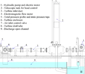
The experimental results to be presented later on were obtained at a facility for testing hydraulic turbines located at the Turbomachinery Laboratory, Instituto Superior Técnico, University of Lisbon, and shown in schematic form in Fig. 1, while Fig. 2 is a photograph of part of the installation. A detailed description of the test rig can be found in Pereira and Borges [13], while Pereira [14] reports some alterations introduced in the experimental set-up, since the completion of the work presented in [13]. For completeness’ sake, a brief summary of the information available in these two references will be presented in the following. In this rig, the water is pumped from a reservoir located below the laboratory floor, to the turbine, passing by a telescopic tank, whose function is to control and maintain constant the head applied to the turbine. After leaving the turbine, the water discharges into an open channel, located again below the laboratory floor, which conducts the water to the underground reservoir from where it was pumped at the beginning.

Fig. 1 – Schematic view of the Cross-Flow turbine

experimental rig.

The power generated in the turbine is absorbed in a DC motor-generator. An inductive torque transducer with a built-in photo-electric speed pick-up is mounted on the turbine axis, allowing the direct measurement of the turbine torque and rotational speed, and so, the measurement of the power generated by the turbine. The turbine enclosure has a valve to control the amount of air that is let in, permitting in this way the creation of a

vacuum pressure inside the enclosure. The value of this vacuum pressure was measured using a pressure transducer. The alterations introduced in the test rig included the modification of the turbine enclosure and some improvements in the instrumentation used to perform the measurements. Indeed, the new turbine enclosure, shown in schematic form in Fig. 3, is larger than the previous one, and is made of stainless steel, with one side panel and the top panel made of perspex, to allow easy visualization of the turbine flow. In terms of instrumentation, the volume flow rate is now measured using an electromagnetic flow meter, located in the inlet duct of the turbine, and some static taps were introduced at inlet to the turbine, to measure the inlet pressure in an alternative way.

Fig. 2 – Photograph of the Cross-Flow turbine

experimental rig.

The pressures are measured using pressure transducers more accurate than the older ones they replace, and the acquisition system was also completely upgraded. In fact, the signals from the several sensors are logged using a personal computer of the type “Pentium IV Celeron”, working at 2.4GHz, with a National Instruments data acquisition board, model PCI-6024E, with a 12-bit resolution, and a maximum sampling rate of

kHz

200 . The data acquisition process was

controlled by a program written in the language “LabView 6.1”. The permissible maximum flow rate and maximum head that can be used in the present test rig, is around 0.1m3 s, and 5.5m, respectively, resulting in a maximum power obtained during the tests to be reported of about

kW 5 .

3 . The tests were performed using turbine rotors with an outside diameter of 300mm, an inside diameter of 200mm, and an internal width of

mm

215 . Most of the results to be presented were

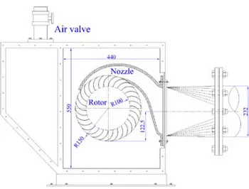
obtained using rotor blades with 1.5mmthickness, although some of the data shown was obtained with a thickness of 3mm for the rotor blades. The nozzle used has an inside width of 210mm, an exit angle of 13°, and an entry arc of 80°. Other dimensions of the turbine are displayed in Fig. 3.

Fig. 3 – Schematic view of the Cross-Flow Turbine.

The results displayed in Fig. 4 show the variation of the turbine efficiency as a function of the blade/jet velocity ratio variation, and were obtained with the turbine configuration that achieved the best performance in all the experimental tests carried out by the authors. The results demonstrate that it is possible to obtain a peak efficiency of 84.8% with a well designed Cross-Flow turbine.

Fig. 4 – Influence of blade-jet velocity ratio on

efficiency.

This peak efficiency was reached for a blade-jet velocity ratio of 0.464, and it should be noted that the geometric parameters of the turbine do not satisfy the relation tan

β

₁=2tan

α

₁, which result from the traditional theoretical model of describing the turbine efficiency.

3 New theory for the turbine

efficiency evolution

As explained in the introductory section, one of the objectives of the present paper is the presentation of new theoretical relations for the efficiency evolution, which is based on a set of approximations similar to the ones traditionally used, with one important exception, that concerning the direction of the flow leaving the rotor. In fact, while in the traditional loss model it is considered that the direction of the flow at the exit of the rotor is a function of the inlet angle,

β

₁, and changes quite a lot when the blade jet velocity ratio, U₁ V₀, varies, in the new theory proposed here, the direction of the flow at rotor exit is assumed constant, independent of U₁ V₀, and equal to the angle of the rotor blades at exit, i.e., for the rotor outside diameter (

β

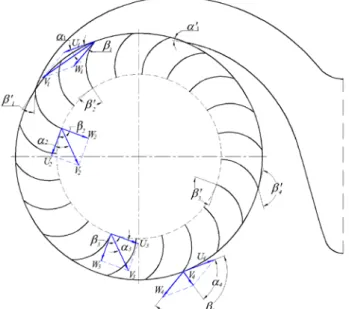
4′).

The explanation of the new theory will be started by a clear enunciation of the approximations that will be assumed to apply to the flow through the turbine. In the present study, the flow is considered one-dimensional passing through a geometry that is schematically shown in Fig. 5, which also displays the assumed velocity triangles at the various stages along the flow (which are the inlet to the first passage, exit of the first passage, inlet to the second passage and exit of the second passage).

Fig. 5 – Cross-Flow turbine geometry and velocity

triangles.

As shown in the figure, the velocity triangles at exit of the first passage and inlet to the second passage are assumed equal, because there is no flow deflection in the rotor inside space and the pressure is constant there. Therefore, the contributions of

these velocity triangles cancel exactly, and, traditionally are not further considered, so that the only velocity triangles analyzed are those at inlet to the first passage and at the exit of the second passage. This conclusion also applies to the case where a fraction of the water never crosses the inside region (never leaves the rotor region with blades). The water flow at exit from the nozzle and from the rotor is also assumed to be well guided by, respectively, the nozzle solid walls and the rotor blades, implying that the angle of the flow issuing from the nozzle is equal to the angle of the nozzle walls at exit (

α

₁ =

α

₁′), and the angle of the relative flow leaving the rotor is equal to the angle of the rotor blades at the rotor outside diameter (

β

4 =

β

4′). In addition, the turbine is considered to be a pure action or impulse turbine, meaning that the pressure only varies inside the nozzle, and is constant at all points of the rotor, similarly to what happens in a Pelton turbine.

The two last conditions fix completely the two relevant velocity triangles (shown in Fig. 6 in detail), and, therefore the energy exchange taking place in the rotor.

Fig. 6 – Detailed velocity triangles.

Indeed, the magnitude of the absolute velocity at the exit of the nozzle (which is coincident with the rotor inlet) is given by:

gH k

V₁= _n 2 (1)

where 2gH =V₀ is the velocity that would exist at nozzle exit if losses were negligible, and k_n is a coefficient smaller than unity, that accounts for the losses occurring inside the nozzle, together with any eventual departures of the flow from the assumption of one-dimensional flow. The magnitude of the relative velocity at exit of the rotor may be estimated using the equation of energy applied to the relative flow, between conditions at inlet and at exit of the rotor, assuming there are no losses (see Vavra [15]), equation that states that:

4 2 4 2 4 4 1 2 1 2 1 1 2 2 g z U W g p z g U W g p + − + = + − + ρ ρ (2)

Realizing that U₁ =U₄ (the exit radius is equal to inlet radius), neglecting the elevation term

(

z1−z4

)

, and invoking again the approximation

that the turbine is an impulse one which implies that 4

1 p

p = , one can conclude that it should be 4

1 W

W = . In order to take into account losses that occur inside the rotor, it will be considered that:

1

4 k W

W = _r (3)

where

k

_r is a coefficient smaller than unity, that accounts for the losses occurring inside the rotor, during the overall passage through the rotor, from point 1 to point 4.

Now, if one applies the Euler’s turbine equation to the present case, it can be said that the energy exchange taking place in the rotor is given by:

θ θ

θ

α

η

gH=U1V1 −U4V4 =U1knV0cos 1′−U4V4 (4) The analysis of the velocity triangles at the exit of the rotor, shown in Fig. 6, enables one to write:

(

4

)

4 4 4

4 4

4θ U W cos

π

β

U W cos

β

V = − − = + (5)

and, since U1 =U4 and W4 =krW1, Eq. (4) leads to:

(

1 1 4

)

1 1 0 1 cos

α

cos

β

η

gH=knUV ′−U U −krW (6)

At this point, the traditional loss model says that 1

4

π

β

β

= − . Instead of that approximation, in the new analysis being proposed, it is considered that

1 1

4

4

β

π

β

π

β

β

= ′ = − ′≠ − (it should be noticed that 1

1

β

β

≠ ′, in general, the difference between these two values being equal to the incidence angle, at inlet to the first passage through the rotor). Fig. 7a) and b) compare the velocity triangles assumed in the traditional and new analysis, for a blade jet velocity ratio of U₁ V₀ =0.9, evidencing the great differences that exist between both theories, chiefly for conditions removed from nominal ones.

While traditionally it is considered that there is a kind of symmetry for the flow angles between inlet and exit of the rotor, in the present analysis no such symmetry exists, since at exit the flow is imposed by the blade geometry near the exit, while at inlet the angle is imposed by the flow. The assumed exit velocity triangles relative to the blade geometry are presented in Fig. 7b), showing that the new proposed approximation considers a plausible exit relative velocity aligned with the blade, while the

traditional model consider an unrealistic exit relative velocity leaving the blade inclined at an appreciable angle relative to the blade.

Fig. 7a) – Comparison of exit velocity triangles for

9 . 0 0 1 V = U .

Fig. 7b) – Comparison of exit velocity triangles for

9 . 0

0 1 V =

U , indicating the rotor blade geometry.

Accepting the approximation

β

₄=

β

₄′ =

π

−

β

₁′, Eq. (6) is transformed into:

(

)

[

0 1 1 1 1

]

1 cos

α

cos

π

β

η

gH =U knV ′−U −krW − ′ (7) The velocity triangles at inlet to the rotor, shown in Fig. 6, allow one to conclude that:

1 0 1 2 1 2 0 2 1 = k V +U −2U k V cosα′ W _{n n} (8)

Substituting this value in Eq. (7), the following expression is obtained:

(

)

1 0 1 2 1 2 0 2 1 1 1 0 1 cos 2 cos cos α β α η ′ − + ′ + + − ′ = V k U U V k k U V k U gH n n r n (9) which, finally, leads to:

    ′ − + ′ +    + − ′ = 1 0 1 2 0 2 1 2 1 0 1 1 0 1 cos 2 cos cos 2 α β α η n n r n k V U V U k k V U k V U (10)

taking into account that V02 =2gH.

Comparing this result with the corresponding expression obtained using the traditional theory and approximations which is:

(

)

_      − + = 1 1 1 1 1 2 cos 1 2 V U V U k kn r α η (11)

several differences become evident. The first one is the fact that the new expression for the efficiency is a lot more complex than the previous one, and now depends on five variables

(

U₁ V₀,

α

₁′,

β

₁′, k_n, k_r

)

while previously there were only four independent variables

(

U₁ V₀,

α

₁, k_n, k_r

)

. This implies that the study of the new expression is much more complex, and, namely, the value of U₁ V₀ that optimizes the efficiency is now given by the solution of the following equation:

(

)

0 cos 2 cos 3 2 cos 2 4 cos 2 1 0 1 2 0 2 1 2 1 0 1 2 0 2 1 2 1 0 1 1 = ′ − +       ′ − + ′ + + − ′ α α β α n n n n r n k V U V U k k V U V U k k V U k (12)

The solution of this equation is not as simple as the result obtained with the traditional model. As a consequence, it is not viable to reach a simple closed algebraic expression for the peak efficiency as was the case with the traditional model which predicts a value of:

(

)

2 cos 1 1 2 2 max α η =kn +kr (13)

However, it is a simple matter to calculate numerically the peak efficiencies as a function of both

α

₁′ and

β

₁′ (instead of only α₁

)

, and the values of blade-jet velocity ratio, U1 V0, at the best

efficiency point. These results are presented in Fig. 8a) and Fig. 8b), respectively. For comparison purposes, in these two figures it is also plotted the curve resulting from the traditional theoretical relation, Eq. (13). In addition, Fig. 8c) shows the

values of the incidence angle at inlet to the rotor, given by

β

₁−

β

₁′, for the best efficiency point.

The study of these graphs indicates that the new theory predicts that the efficiency is more influenced by the value of β ′ than 1 α′ , and in the 1

range of α′ normally used, the predicted peak ₁ efficiency by the new model is greater than the values obtained with the traditional model, and is not limited by the curve defined by Eq. (13). Note also that the new model predicts that for a constant value of α′ , the efficiency increases when the value ₁ of β ′ decreases. This prediction is in clear 1

contradiction with the traditional model that state that the efficiency does not depend on β ′, and ₁ anticipate that for maximum efficiency (obtained by a mathematical optimization, done by differentiating Eq. (11)), the relation:

1 1 2tg

tg

β

=

α

(14)

should apply.

Fig. 8a) – Theoretical peak efficiency, function of α₁′

and β₁′.

Fig. 8b) – Theoretical blade-jet velocity ratio at best

efficiency point.

In order to quantify this contradiction some typical values can be advanced. In fact, it can be

seen in Fig. 8a) that the new analysis predicts an increase of 2.8% in efficiency when the angle β ′ is 1

decreased from a value of 30° to a value of 20°, for an angle at exit of the nozzle equal to α1′ 13= °

(assuming loss coefficients of k_n =k_r =0.9), while the traditional model predicts that the maximum efficiency occurs when

β

₁=arctan

(

2tan

α

₁

)

=24,8° (given by Eq. (14)), and does not depend on β ′ . 1

Fig. 8c) – Theoretical incidence angle at inlet to the rotor,

at best efficiency point.

A comparison between these theoretical predictions and experimental results could help us identify the analysis that best describes the reality. This comparison is done in Fig. 9a), where the measured efficiency curve obtained with two Cross-Flow turbines which only differ in the value of β₁′ used in the rotors is presented - for one rotor it is

° = ′ 30

1

β , and for the other is β1′ 20= °, and the

nozzle is the same, with a nozzle exit angle,

α

₁

′

, of °

13 . Fig. 9b) shows a similar example, where this time the angle β₁′ was varied between the values of

°

20 and 15°, using thinner blades than in the rotors considered in Fig. 9a) (in the rotors of Fig. 9a) the thickness of the blades is equal to 3 mm, while in Fig. 9b) the blade thickness is 1.5 mm). In both tests, the head used was equal to 3.1 m.

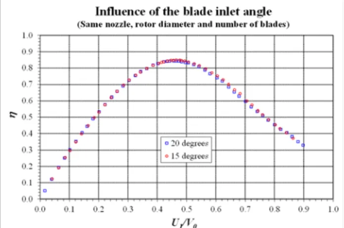
Fig. 9a) – Influence of the inlet rotor angle, β₁′, on the measured efficiency (blade thickness of 3 mm).

The difference in peak efficiency detected in Fig. 9a) is 1.4%, and in Fig. 9b) is 0.5%. These two plots clearly show that the value of β ′ does 1

influence the efficiency curves and the peak efficiency values. In accordance with the theoretical predictions of the new model, the value of peak efficiency increases as the angle β ′ decreases, ₁ although for the smaller values of β ′, the gains ₁ achieved in the peak efficiency are quite small and marginal. Perhaps, more significant that the previous conclusion is the fact that the predictions of the traditional model are not borne out by the experimental data, since the peak efficiency value does show a clear dependency on the value of the rotor inlet angle, β ′, and the best performance does 1

not occur for a value of β ′ between ₁ 20° and 30° as Eq. (14), anticipates based on a “mathematical optimization” (

β

₁=arctan

(

2tan

α

₁

)

=24,8°), but, rather, for the smaller value of β₁′ that was tested

(

β1′ 15= °

)

. This result, besides clearly showing the

shortcomings of the traditional theoretical relations, also means that the turbine designer that would accept the constraint expressed in Eq. (14) (and it should be noted that most authors do accept this constraint) would necessarily end up with a turbine that has a peak efficiency which is not as high as it could have been. Based on the arguments presented herewith, it seems safe to conclude that the inlet rotor angle, β ′ , should be chosen as small as 1

physically possible, and Eq. (14) should be discarded. This is a radical departure from what has been the traditional wisdom when designing Cross-Flow turbines.

Fig. 9b) – Influence of the inlet rotor angle, β₁′, on the measured efficiency (blade thickness of 1.5 mm).

When doing the above recommendation, it is recognized that the use of rotor inlet angles, β ′, that 1

do not obey Eq. (14) lead to incidence angles at inlet to the rotor that are in absolute value larger than zero, as is clearly displayed in Fig. 8c). These larger incidence angles should imply larger incidence losses, which are not taken into account in the present analysis. However, the experimental results seem to suggest that this increased level of incidence losses is not of sufficient magnitude to declare invalid or change significantly the above conclusions and recommendations.

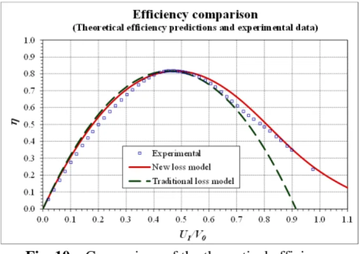
Another comparison carried out between the theoretical predictions and the experimental data done with the intention of assessing the validity of the new analysis is presented in the next figure, Fig. 10, where the predictions of the traditional and the new efficiency relations are plotted against a typical set of experimentally measured points, obtained with a Cross-Flow turbine that have a nozzle exit angle, α′ , equal to ₁ 13°, a rotor inlet angle,β ′ , equal to ₁ 30°, and 30 blades. Both analyses depend on two parameters (loss coefficients k and n k ), which need to be r estimated, before being able to draw the curves representing them. The value of k was chosen _n

based on an estimate of the energy losses inside the nozzle and non-uniformity of the flow at the rotor inlet, and was considered equal to 0.938 for both models. The values of the loss coefficient k were _r

adjusted so that the predicted peak efficiency value was equal to the experimental value (81.8%). This procedure resulted in a loss coefficient, k , of 0.956 r for the traditional model and a value of 0.998 for the new model.

Fig. 10 – Comparison of the theoretical efficiency

predictions with experimental data.

Comparing both theoretical curves, it is seen that the biggest differences occur for the larger values of

the blade-jet velocity ratio, U₁ V₀, with the curve for the new analysis showing a large asymmetry around the best efficiency point, while the curve representing the traditional theoretical relation is symmetric. It should also be noticed that the traditional theory predicts that the efficiency goes to zero (situation corresponding to the run-away speed) for a blade-jet velocity ratio, U₁ V₀ smaller than 1.0 (see Fig. 10), in clear contrast with the expectations of the new analysis, and the experimental results, since for the measured point with the largest blade-jet velocity ratio (U1 V0 roughly equal to 1.0) the measured efficiency is near 20%. This indicates that the run-away speed occurs for values of the blade-jet velocity ratio, U₁ V₀, greater than 1.0, according to the predictions of the new theory. The graph also shows that the curve describing the new theoretical relation fits better the experimental results than the curve representing the traditional model, specially for the larger values of the blade-jet velocity ratio,

0 1 V

U . It is also significant that the new analysis always indicates values of efficiency slightly greater than the measured points, a fact that can be explained with the extreme simplicity of the new proposed theoretical analysis, which neglects some losses that may be important in reality. One of these losses is the possible additional loss due to a large angle of incidence at inlet to the rotor, that may cause some local perturbations and separations because the rotor blades are very thin and the leading edges are quite sharp. This fact may account, at least partially, for some of the differences seen in Fig. 10 between the curve of the new theoretical analysis and the experimental results, see also Fig. 8c).

Other effects not considered in the present analysis result from the approximations accepted at the start of the present analysis that may be not exactly satisfied. This is the case with the assumption that the turbine is a pure action or impulse turbine, which is known not to be true for some combinations of the geometric parameters, and for the larger values of blade-jet velocity ratio,

0 1 V

U , see [2, 3, 14, 16], for example. This fact seems to influence the values of the blade-jet velocity ratio, U₁ V₀, where the best efficiency point is located, since these values are not well predicted by the new theoretical analysis.

Another approximation that may be not exactly verified concerns the value of the angle of the relative flow at exit to the rotor, which may not be exactly equal to

β

₄′, as assumed here. In fact, some

experimental results recently published elsewhere [12], seem to suggest that there is a deviation between the angle of the relative flow leaving the rotor and the blade angle,

β

₄′, which is roughly constant and independent of the blade-jet velocity ratio, U₁ V₀. If this is the case, the above new theoretical relation still applies, provided one is careful enough to substitute the value of the rotor blade exit angle,

β

4′, with the actual angle of the relative flow, which is equal to

β

4′−∆

β

, where ∆

β

is the supposed constant deviation between the two angles just indicated. According to [12], the magnitude of the deviation ∆

β

is of the order of

°

15 for the particular geometry tested. This correction should be implemented using the angle

1

β ′ instead of

β

4′, implying that the numeric values of β ′ should be substituted by ₁ β₁′+∆β , in Figs. 8, resulting in a reduction of the peak efficiency values, as should be expected. A similar reasoning also applies to the flow issuing from the nozzle, where instead of using the value of the angle of the nozzle walls at exit, α′ , one should use the true ₁ angle of the absolute flow leaving the nozzle

(

α₁′+∆α

)

.

4 Conclusion

A study about several aspects concerning the efficiency of a Cross-Flow turbine is described in this paper, leading to the presentation of typical experimental efficiency values and of a new theoretical analysis for the prediction of the efficiency evolution. The experimental results described also demonstrated that a peak efficiency value of 84.8% is attainable with this kind of turbine.

In the second part of the paper, a critical appraisal of previous theoretical analyses was carried out, indicating that there is an important flaw in the reasoning behind most of the published theoretical relations, since the angle of the relative flow at rotor exit used is

β

4 =

π

−

β

1, which varies a lot with the blade-jet velocity ratio, U₁ V₀, while, in reality, it should remain nearly constant, and should be related to the rotor blade exit angle,

β

₄′. A new theoretical analysis that corrects this flaw is proposed here, and the consequences were explored. It is shown that the new analysis predicts a peak efficiency that also depends on the inlet rotor angle, β ′ , and that it 1

describes more adequately the experimental data, validating its use. In terms of turbine design, it is

defended here that the inlet rotor angle, β ′ , should ₁ be chosen as low as physically possible, and not according to the expression tan

β

1=2tan

α

1, which is an expression relating the nozzle exit angle with the inlet rotor angle widely accepted in the published literature.

Acknowledgements:

The authors gratefully acknowledge the financial support granted by Fundação para a Ciência e Tecnologia (project PTDC/ECM/73867/2006), as well as the assistance given by IDMEC/LAETA, IST-Universidade Lisboa and ESTSetúbal/IPS.

References:

[1] Mockmore, C. A., and Merryfield, F., The Banki water turbine, Bulletin Series Nº 25, Engineering Experimental Station, Oregon State System of Higher Education, Oregon State College, Corvalis, USA, 1949, pp. 4-27. [2] Varga, J., Tests with the Bánki water turbine,

Acta Technica Academicae Scientiarum Hungaricae, Vol. 27, Nº1-2, 1959, pp. 79-102.

[3] Nakase, Y., Fukutomi, J., Watanabe, T., Suetsugu, T., Kubota, T., and Kushimoto, S., A study of Cross-Flow turbine (Effects of nozzle shape on its performance), Proc. ASME

Conference on Small Hydro-Power Fluid Machinery, Phoenix, Arizona, USA, November

14-19, 1982, pp. 13-18.

[4] Johnson, W., Ely, R., White, F., Design and testing of an inexpensive Cross-Flow turbine,

Proc. ASME Conference on Small Hydro-Power Fluid Machinery, Phoenix, Arizona,

USA, November 14-19, 1982, pp. 129-133. [5] Van Dixhorn, L. R., Moses, H. L., and Moore,

J., Experimental determination of blade forces in a Cross-Flow turbine, Proc. ASME

Conference on Small Hydro-Power Fluid Machinery, New Orleans, Louisiana, USA,

December 9-14, 1984, pp. 67-75.

[6] Khosrowpanah, S., Fiuzat, A. A., Albertson, M. L., Experimental study of Cross-Flow turbine,

Journal Hydraulic Engineering, Vol.114, Nº3,

1988, pp. 299-314.

[7] Desai, V. R., and Aziz, N. M., Parametric evaluation of Cross-Flow turbine performance,

Journal of Energy Engineering, Vol.120, Nº1,

1994, pp. 17-34.

[8] Totapally, H. G. S., and Aziz, N. M., “Refinement of Cross-Flow turbine design

parameters,” Journal of Energy Engineering, Vol.120, Nº3, 1994, pp. 133-147.

[9] Olgun, H., Investigation of the performance of a Cross-Flow turbine, International Journal of

Energy Resources, Vol.22, 1998, pp. 953-964.

[10] Csanady, G. T., Theory of Turbomachines, McGraw-Hill Book Co., New York, USA, pp. 122, 1964.

[11] Dixon, S. L., Fluid Mechanics and

Thermodynamics of Turbomachinery, 4th ed.,

Butterworth-Heinemann, Boston, pp. 145, 1998.

[12] Borges, J. E., Costa Pereira, N. H., Matos, J., and Frizell, K. H., Performance of a combined three-hole conductivity probe for void fraction and velocity measurement in air–water flows,

Experiments in Fluids, Vol.48, 2010, pp. 17-31.

[13] Costa Pereira, N. H., and Borges, J. E., Study of the nozzle flow in a Cross-Flow turbine,

International Journal of Mechanical Sciences,

Vol. 38, Nº3, 1996, pp. 283-302.

[14] Costa Pereira, N. H., Estudo de uma Turbina ‘Cross-Flow’, Ph.D. thesis, Technical University of Lisbon, Lisbon, Portugal (in Portuguese) , 2007.

[15] Vavra, M. H., Aero-Thermodynamics and Flow

in Turbomachines, John Wiley & Sons Inc,

New York, USA, pp. 123-125, 1960.

[16] Haimerl, L. A., The Cross-Flow turbine, Water