Ultrasonic Guided Waves for Structural Health Monitoring and Application to Rail Inspection Prototype for the Federal Railroad Administration

(1)

Dottorato di Ricerca in

Ingegneria dei Materiali e delle Strutture

- Ciclo XX -

Ultrasonic Guided Waves for Structural Health Monitoring and

Application to Rail Inspection Prototype for the

Federal Railroad Administration

by

Stefano Coccia

A dissertation submitted in fulfillment

of the requirements for the degree of

Doctor of Philosophy

ADVISOR

Professor Erasmo Viola

CO-ADVISOR

Professor Francesco Lanza di Scalea

PhD. COORDINATOR

Professor Domenico Bruno

(2)

ii

The dissertation of Stefano Coccia is approved:

25.11.07 _________________________________________________________

Professor Domenico Bruno Date

25.11.07 ________________________________________________________

Professor Erasmo Viola Date

_________________________________________________________ Date

Università della Calabria, Rende

November 2007

(3)

iii

Ultrasonic Guided Waves for Structural Health Monitoring and Application to Rail Inspection Prototype for the

Federal Railroad Administration

(4)

iv

Ultrasonic Guided Waves for Structural Health Monitoring and Application to Rail Inspection Prototype for the

Federal Railroad Administration by

Stefano Coccia

Recent train accidents, associated direct and indirect costs, as well as safety concerns, have reaffirmed the need for developing rail defect detection systems more effective than those used today. Current methods for detecting internal flaws in rails rely primarily on ultrasonic pulse-echo technology operated in a water-filled wheel or sled. Presence and loss of echoes along each tested direction are analyzed in parallel to map surface and internal cracks in the rail. While this technology has served the industry well, several inherent weaknesses exist. Contact heads and cross-sectional inspection limit the speed of the measurement; liquid couplant is required to maintain efficient wave/echo transmission through the contact patch. Despite the acoustic couplant, significant transmission loss results from the pulse/echo passing through the contact patch twice. More importantly, ultrasonic beams launched vertically from the top of the rail head can miss internal defects located under horizontal shelling; this was the case, in the disastrous train derailment at Superior, WI in 1991. As a proposal to address these issues, the use of ultrasonic guide waves appears promising. One objective of this work is extending the fundamental knowledge of the guided

(5)

v

frequency (<500 kHz) range. The selection of guided wave features sensitive to the presence of the different type of defects is essential for a successful defect detection performance. Another accomplishment of this work is the development of a rail defect detection prototype based on a laser/air-coupled ultrasonic technique. The prototype has been successfully tested twice in the field for the Federal Railroad Administration in the United States of America and it shows promise for implementation in rail inspection cars.

(6)

vi

“If a man empties his purse into his head, no man can take it away from him.

An investment in knowledge always pays the best interest.”

(7)

vii

I am forever grateful for the opportunity to perform this research under the guidance of my advisors, Prof. Erasmo Viola with the University of Bologna Department of Structural Engineering (D.I.S.T.A.R.T., UNIBO) and Prof. Francesco Lanza di Scalea with the Department of Structural Engineering of University of California San Diego (UCSD), USA. Their selfless support and academic passion were critical for the success of my research. I would like to specially thank Prof. Domenico Bruno and the doctorate committee members with the University of Calabria Structural Engineering Department (Dipartimento di Strutture, UNICAL), for giving me the possibility of spending an extended period of research in UCSD. Thanks go to my colleagues in the Laboratory of Computational Mechanics (LAMC) of UNIBO, Prof. Alessandro Marzani and Dr. Giovanni Castellazzi and to my colleagues in the NDE/SHM Laboratory of UCSD, Dr. Salvatore Salamone, Dr. Howard Matt, and especially Dr. Ivan Bartoli for their invaluable contributions, humor and friendship. A special thank goes to Prof. Piervincenzo Rizzo for the exceptionally helpful collaboration in producing the results shown in chapter 4.

The research presented in this dissertation was supported by the Federal Railroad Administration (FRA) of the U.S. Department of Transportation, under university research grant DTFR53-02-G-00011. The work was sponsored by FRA‟s Office of Research and Development. The author is grateful to Mahmood Fateh, FRA‟s Technical Representative, for his technical guidance and valuable comments during the different phases of the research, and to Gary Carr, formerly Senior Engineer of

(8)

viii

technical and logistic support during the prototype assembling and field testing. The in-kind support of San Diego Trolley, Inc. which donated parts of the rail specimens used for testing purposes to the NDE & SHM Laboratory at UCSD, is acknowledged. The research was also partially funded by the UCSD/Los Alamos Cooperative Agreement on Research and Education (CARE), for which the author is thoroughly appreciative. Thanks are extended to Dr. Gyuhae Park and Prof. Charles Farrar for the established fruitful collaboration.

A special thank goes to all the people who have been supportive over these years of research work, first of all my family; without them I would not have been able to accomplish this task.

Part of chapter 4 of this dissertation was printed in Insight –Non –Destructive

Testing & Condition Monitoring, Lanza di Scalea, F., Rizzo, P., Coccia, S., Bartoli, I.,

Fateh, M., Viola, E. and Pascale, G., 2006. “Non-Contact Ultrasonic Inspection of Rails and Signal Processing for Automatic Defect Detection and Classification”. The dissertation author was co-author of this paper. A segment in chapter 4 has been published in Insight - Non-Destructive Testing & Condition Monitoring, Rizzo, P., Bartoli, I., Cammarata, M. and Coccia, S., 2007. “Digital signal processing for rail monitoring by means of ultrasonic guided waves.” The dissertation author was co-author of this paper. Chapter 5, in part, has been published in Transportation

Research Record, Journal of the Transportation Research Board, Lanza di Scalea, F.,

(9)

ix

The dissertation author was co-author of this paper. An additional part in chapter 5 was presented at World Forum on Smart Materials and Smart Structures Technology, Coccia, S., Bartoli, I., Lanza di Scalea, F., Rizzo, P., Fateh, M. and Yang, T.-L., 2007. “Non-contact Ultrasonic Rail flaw Detection”. The dissertation author was the main contributor of this paper. A section in chapter 5 was presented at IWSHM - The 6th International Workshop Structural Health Monitoring, Coccia, S., Bartoli, I., Lanza di Scalea, F., Rizzo, P. and Fateh, M., 2007. “Non-contact Ultrasonic Rail Defect Detection System. Prototype development and field testing”. The dissertation author was the main contributor of this paper. An additional segment in chapter 5 is in

Technical Report for the University of San Diego, California, Rizzo, P., Coccia, S.,

and Lanza di Scalea, F., 2005. “On line High-Speed Rail Defect Detection, Final Report-Phase III”. The dissertation author was co-author of this paper. In part, chapter 5 was in Technical Report for the Federal Railroad Administration, Coccia, S., Bartoli, I., Lanza di Scalea, F. and Rizzo, P., 2007. “Non-contact Rail Defect Detection: First and Second Field Tests”. The dissertation author was the main contributor of this paper. Chapter 3, in part, will be submitted for publication in

Journal of Acoustical Society of America, Coccia, S., Bartoli, I., Lanza di Scalea, F.,

Marzani, A., 2008. The current running title of this paper is “Forced solution of guided waves in rails”. The dissertation author is the primary investigator and author of this paper.

(10)

x

Signature Page ...ii

Abstract … ... iv

Epigraph…. ... vi

Acknowledgments ...vii

Table of Contents ... x

List of Figures ... xv

List of Tables ...xxvii

1 Introduction ... 1

1.1 Health monitoring of railroad tracks.Introductory discussion and motivation for research ... 1

1.2 Outline of the numerical and experimental approach of the ... 2

2 State of the art review ... 4

2.1 Description of various structural defect in rails ... 4

2.1.1 Rail manufacturing defects ... 7

2.1.2 Rail defects caused by improper use or bad maintenance ... 13

2.1.3 Rail defects due to wearing mechanisms of the rolling surfaces and to fatigue (Rolling Contact Fatigue – RCF defects) ... 16

2.2 Current rail inspection systems ... 24

2.2.1 Historical background ... 24

(11)

xi

2.3.1 Guided wave advantages for rail inspection ... 34

2.3.2 Laser generation of ultrasonic guided waves ... 35

2.4 Modeling guided wave propagation in rails ... 37

3 Modeling ultrasonic wave propagation in waveguides of arbitrary cross-section ... 40

3.1 Introduction ... 40

3.2 Guided Waves in an unbounded medium ... 40

3.3 Guided waves in a bounded medium. Case of a single isotropic plate ... 43

3.4 Semi Analytical Finite Element Method ... 47

3.4.1 SAFE Mathematical Framework ... 49

3.4.2 Modeling the attenuation in the rail ... 56

3.4.3 Rail as undamped waveguide ... 58

3.4.4 Group and energy velocity ... 60

3.4.5 Methods to accelerate the SAFE solution process ... 61

3.5 Unforced solution of guided waves in rails ... 66

3.6 Forced solution for guided waves in rails ... 81

3.7 Response of the rail to a laser excitation ... 87

3.7.1 Mode tracking algorithm ... 102

3.7.2 Distribution of in-plane strain energy in the rail cross-section ... 104

(12)

xii

3.8 Conclusions ... 129

4 Defect-sensitive feature extraction from ultrasonic waves ... 130

4.2 Continuous and discrete wavelet analysis ... 131

4.2.1 Theory behind wavelet analysis ... 133

4.2.2 Discrete Wavelet Transform (DWT) analysis for signal decomposition ... 136

4.2.3 DWT for Data De-noising and High Speed Data Manipulation144 4.3 Digital processing of ultrasonic signals ... 148

4.3.1 Digital filtering ... 148

4.3.2 Spatial averaging algorithm for enhancement of defect detection in “reflection mode” ... 149

4.4 Feature extraction in ultrasonic rail inspection ... 162

4.4.1 Joint time-frequency domain feature extraction ... 162

4.4.2 DWT-based feature extraction. A synopsis of univariate and multivariate approaches ... 172

4.4.3 Feature extraction for Energy Normalized D.I. computation ... 175

4.5 Validation of signal processing for defect detection in rails ... 178

4.5.1Introduction ... 178

(13)

xiii

4.6 Conclusions ... 197

5 Development of Rail Inspection Prototype for the Federal Railroad Administration ... 198

5.2 Stage I: Hardware and Software ... 199

5.2.1 Q-Switched laser generator and optical elements ... 199

5.2.2 Air-coupled Transducers and Preamplifiers ... 202

5.2.3 D.I. Computation ... 204

5.2.4 Hardware Controller and DAQ Boards ... 207

5.2.5 Software implementation ... 210

5.3 Stage II. Prototype deployment ... 229

5.3.1 Hardware layout ... 229

5.3.2 Software implementation ... 232

5.4 Stage III. Prototype upgrade ... 243

5.4.1 New cart ... 243

5.4.2 Improved sensor arrangement ... 244

5.4.3 Software upgrade ... 247

5.5 Field testing ... 249

5.5.1 First field test ... 249

(14)

xiv

6 Conclusions ... 278

6.1 Review of the dissertation and summary of the results ... 278

6.2 Recommendations for future work ... 280

(15)

xv

Figure 2.1: Rail defects, operational restrictions and remedial actions for the U.S.

Departments of Army ... 5

Figure 2.2: Relative position of planes through a rail ... 7

Figure 2.3: Appearance of different cases of transverse defects ... 8

Figure 2.4: Transverse defects. Case of coupling with shelling ... 9

Figure 2.5: General appearance of an horizontal split head ... 10

Figure 2.6: General appearance of a vertical split head ... 11

Figure 2.7: Case of a head/web separation ... 11

Figure 2.8: General appearance of a piped rail ... 12

Figure 2.9: Sketch of cases of mill defects ... 13

Figure 2.10: General appearance of a split web ... 13

Figure 2.11: Sketch of an engine burn ... 14

Figure 2.12: General appearance of engine burn fractures ... 14

Figure 2.13: Sketch of a crushed head ... 15

Figure 2.14: Sketch of a case of torched cut rail ... 15

Figure 2.15: Contact stresses on tight curved track ... 16

Figure 2.16: Example of the broken base defect ... 17

Figure 2.17: Sketches of bolt hole cracks ... 18

(16)

xvi

Figure 2.20: General appearance of the end batter defect ... 20

Figure 2.21: Sketch of the flaking phenomenon ... 21

Figure 2.22: General appearance of rail wear ... 22

Figure 2.23: Example of shelling ... 23

Figure 2.24: Trapped fluids causing cracking to worsen ... 23

Figure 2.25: Ultrasonic probe wheel transducer arrangements ... 27

Figure 2.26: Scheme of the contact induction technique ... 28

Figure 2.27: Guided waves propagating within a confined geometry. ... 31

Figure 2.28: Rail defect detection: “long-range method” ... 34

Figure 2.29: Laser generation of ultrasound in (a) thermoelastic regime and (b) ablative regime. ... 46

Figure 3.1: Guided wave propagation within a thin isotroipc plate ... 43

Figure 3.2: Waveguide in vacuum: infinitely wide plate. ... 49

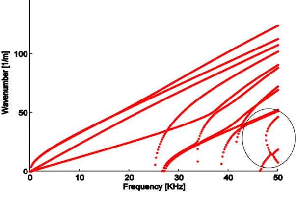
Figure 3.3: Dispersion curves of a 115 lb A.R.E.M.A. section rail; high frequency resolution is needed to correctly interpret the solutions in proximity of two modes ... 62

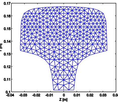
Figure 3.4: Mesh of the rail cross section generated by ABAQUS™ ... 67

Figure 3.5: Wavenumbers as a function of frequency ... 68

Figure 3.6: Phase velocity dispersion curves ... 69

Figure 3.7: Mode filtering by thresholding the phase velocity ... 71

(17)

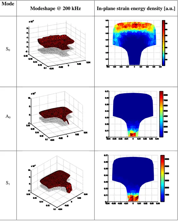
xvii Figure 3.10: Modeshape of S0 at 200 kHz ... 73 Figure 3.11: Modeshape of A0 at 200 kHz ... 74 Figure 3.12: Modeshape of S1 at 200 kHz ... 75 Figure 3.13: Modeshape of A1 at 200 kHz ... 76 Figure 3.14: Modeshape of S2 at 200 kHz ... 77 Figure 3.15: Modeshape of A2 at 200 kHz ... 78 Figure 3.16: Modeshape of S3 at 200 kHz ... 79 Figure 3.17: Modeshape of A3 at 200 kHz ... 80

Figure 3.18: Time and frequency domain of the load function ... 88

Figure 3.19: Wavenumbers as a function of frequency in undamped rail. ... 89

Figure 3.20: Phase velocity dispersion curves in undamped rail ... 91

Figure 3.21: Group velocity dispersion curves in undamped rail ... 93

Figure 3.22: Frequency domain displacement of the central node of the top of the railhead subjected to laser excitation at 4” (≈ 102 mm) away from the node ... 95

Figure 3.23: Time domain displacement of the central node of the top of the railhead subjected to laser excitation at 4” away from the node ... 96

Figure 3.24: Laser-generated signal acquired by the air-coupled sensor ... 97

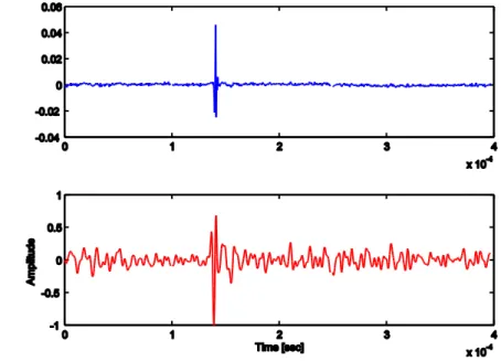
Figure 3.25: Raw simulated(red) and 40 kHz high-passed(blue) simulated response ... 98

Figure 3.26: Raw and 500 kHz low-passed experimental signals ... 98

Figure 3.27: Comparison of the measured response with the results of the SAFE simulation ... 99

(18)

xviii

Figure 3.29: Phase velocity dispersion curves filtering. ... 101 Figure 3.30: Wavenumber as a function of frequency for damped rail. Case of double

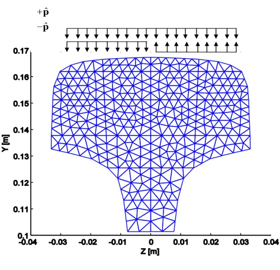
solutions ... 104 Figure 3.31: Symmetric excitation pattern on the meshed rail section ... 111 Figure 3.32: Nonsymmetric excitation pattern on the meshed rail section ... 112 Figure 3.33: Mode excitability curves for a case of symmetric excitation of the rail

head ... 114 Figure 3.34: Mode excitability curves for a case of nonsymmetric excitation of the

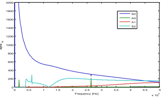
rail head ... 116 Figure 3.35: S0, A0, A1 and S2 mode excitability curves for a symmetric excitation of

the rail head ... 118 Figure 3.36: S0, A0, A1 and S2 mode excitability curves for a nonsymmetric excitation

of the rail head ... 118 Figure 3.37: Nonsymmetric load as sum of symmetric and antisymmetric

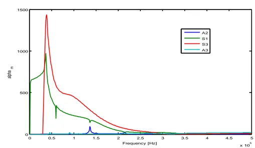
contributions ... 119 Figure 3.38: S1, A2, S3 and A3 mode excitability curves for a symmetric excitation of

the rail head ... 121 Figure 3.39: S1, A2, S3 and A3 mode excitability curves for a nonsymmetric excitation

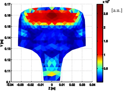
of the rail head ... 121 Figure 3.40: In-plane cross sectional strain energy distribution for a symmetric

excitation at 4” (≈ 102 mm) from the source ... 122

Figure 3.41: In-plane cross sectional strain energy distribution for a nonsymmetric excitation at 4” (≈ 102 mm) from the source ... 122 Figure 3.42: Maximum of the signal envelope acquired at different distances from the

(19)

xix

Figure 3.44: In-plane cross sectional strain energy distribution for a symmetric excitation at 6” (≈ 152mm) from the source ... 125 Figure 3.45: In-plane cross sectional strain energy distribution for a nonsymmetric

excitation at 2” ≈ 51 mm) from the source ... 125 Figure 3.46: In-plane cross sectional strain energy distribution for a nonsymmetric

excitation at 6” (≈ 152 mm) from the source ... 126 Figure 3.47: Cross sectional in-plane strain energy of rail response, filtered with a 300

kHz, 3-order Butterworth highpass ... 128 Figure 3.48: Cross sectional in-plane strain energy of rail response, filtered with a

100-300 kHz, 3-order Butterworth bandpass ... 129 Figure 4.1: The Gabor wavelet with 2 and Gs = 5.34. (a) Time domain, real

and imaginary components. (b) Magnitude of Fourier spectrum ... 136 Figure 4.2: Wavelet spectra resulting from scaling of the mother-wavelet in the time

domain ... 139 Figure 4.3: Replacement of an infinite wavelet set by one scaling function ... 140 Figure 4.4: (a) Discrete Wavelet filter-bank decomposition; (b) signal reconstruction

from wavelet coefficients; (c) reconstruction of original signal ... 144 Figure 4.5: Example of discrete wavelet processing. (a) Unprocessed signal; (b), (c)

wavelet coefficient vector of levels cD3, cD4, and cD5 relative to the direct and the echo signal, respectively; (d), (e) thresholded wavelet coefficient vectors in (b) and (c), respectively; (f) and (g) reconstructed direct and echo signals, respectively, using the thresholded wavelet coefficient vectors in (d) and (e). ... 145 Figure 4.6: Detection scheme for coherent acquisition of guided waves reflected by a

(20)

xx

Figure 4.8: Probe spacing and laser-beam position relative to the defect ... 152 Figure 4.9: Waterfall plot of ultrasonic signals acquired in proximity of the 8 mm

deep surface defect ... 152 Figure 4.10: Mesh of the reflected waves extracted from the 12 A-scans acquired in

proximity of the 8 mm deep surface defect ... 153 Figure 4.11: CWT of the first A-scan acquired in proximity of the 8 mm deep surface

defect ... 154 Figure 4.12: Waterfall plot of the 12 A-scans acquired in proximity of the 23% H.A.

reduction internal defect ... 155 Figure 4.13: A-scans acquired in proximity of the third internal defect, high-passed at

100 kHz ... 156 Figure 4.14: Zoom in, of the waveforms reflected from the 23% H.A. reduction

internal defect ... 157 Figure 4.15: Mesh of the reflected waves extracted from the 12 A-scans acquired in

proximity of the 23% H.A . reduction internal defect ... 158 Figure 4.16: Mesh of the reflected waves extracted from the 12 A-scans acquired in

proximity of the 23% H.A . reduction internal defect, after the application of the spatial averaging technique ... 159 Figure 4.17: CWT of the first A-scan using the Gabor motherwavelet ... 160 Figure 4.18: CWT of the first A-scan using the Complex Morlet 1-1 motherwavelet ... 160 Figure 4.19: Front and 3-D view of the rail head with the 23% H.A. reduction internal

flaw ... 161 Figure 4.20: Defect detection schemes examined. “Reflection mode” with a single

air-coupled sensor (top); “transmission mode” with a pair of air-coupled sensors (bottom). ... 163

(21)

xxi

Figure 4.22: Feature-based Damage Index as a function of the center crack depth monitored in the “reflection mode”; (a) variance of the wavelet coefficients; (b) area of the frequency spectrum of the reconstructed signal; (c) maximum amplitude of the Hilbert transform of the reconstructed signal ... 167 Figure 4.23: Feature-based Damage Index as a function of the corner crack depth

monitored in the “reflection mode”; (a) variance of the wavelet coefficients; (b) area of the frequency spectrum of the reconstructed signal; (c) maximum amplitude of the Hilbert transform of the reconstructed signal ... 168 Figure 4.24: Feature-based Damage Index as a function of the center crack depth

monitored in the “transmission mode”; (a) variance of the wavelet coefficients; (b) area of the frequency spectrum of the reconstructed signal; (c) maximum amplitude of the Hilbert transform of the reconstructed signal ... 170 Figure 4.25: (a) Photo of the rail track up at UCSD; (b) schematic of the

mock-up layout; (c) defect detection scheme in „transmission mode‟ with a pair of air-coupled transducers ... 179 Figure 4.26: Rail defect detection prototype deployed on the rail track mock-up at

UCSD ... 181 Figure 4.27: Typical waveforms detected by the hybrid laser/air-coupled transducer

system. (a), (b) Time waveforms detected by the rear and front sensors, respectively, when the inspection system is probing a damage–free rail; (c), (d) time waveforms detected by the rear and front sensors, respectively, when the inspection system is probing a 5% HA transverse surface notch; (e), (f) time waveforms detected by the rear and front sensors, respectively, when the inspection system is probing a joint ... 182 Figure 4.28: (a) The Coiflet wavelet of order 4; (b) the Symlet wavelet of order 6; (c)

(22)

xxii

system is probing a transverse surface notch; (c), (d) wavelet coefficient vector of detail levels 2 and 3 relative to the rear and front sensors, respectively; (e), (f) reconstructed rear and front sensor signals, respectively, using the thresholded (empty circles) wavelet coefficient vectors in (c) and (d) ... 186 Figure 4.30: (a) RMS-based Damage Index as a function of the acquisition number

for the unprocessed time waveforms, the vector of the retained wavelet coefficients, and the time-domain reconstructed (de-noised) signal; (b) detail plot of (a) ... 187 Figure 4.31: (a) RMS-based Damage Index as a function of the acquisition number

calculated for four different wavelet coefficients vectors; (b) detail plot of (a) ... 189 Figure 4.32: (a) RMS-based Damage Index as a function of the acquisition number

for the vector of the threshold wavelet coefficients, computed from three different mother wavelets; (b) detail plot of (a) ... 190 Figure 4.33: Typical waveforms filtered with the 300-1,100 kHz pass-band

Butterworth. (a), (b) Time waveforms detected by the rear and front sensors, respectively, when the inspection system is probing a damage– free rail; (c), (d) time waveforms detected by the rear and front sensors, respectively, when the inspection system is probing a transverse surface notch; (e), (f) time waveforms detected by the rear and front sensors, respectively, when the inspection system is probing a joint ... 192 Figure 4.34: Typical waveforms filtered with the 40-300 kHz pass-band Butterworth.

(a), (b) Time waveforms detected by the rear and front sensors, respectively, when the inspection system is probing a damage–free rail; (c), (d) time waveforms detected by the rear and front sensors, respectively, when the inspection system is probing a transverse surface notch; (e), (f) time waveforms detected by the rear and front sensors, respectively, when the inspection system is probing a joint ... 193 Figure 4.35: Damage Index as a function of the acquisition number, based on (a)

(23)

xxiii

Figure 4.36: Damage Index as a function of the acquisition number, based on (a) normalized RMS of the signal amplitudes and (b) temporal signal coherence. Sensors deployed on the Gage Side of the rail and signals filtered with a pass-band 300-1,100 kHz third order Butterworth ... 194 Figure 4.37: Damage Index as a function of the acquisition number, based on (a)

normalized RMS of the signal amplitudes and (b) temporal signal coherence. Sensors deployed on the Center Head of the rail and signals filtered with a pass-band 40-300 kHz third order Butterworth ... 196 Figure 4.38: Damage Index as a function of the acquisition number, based on (a)

normalized RMS of the signal amplitudes and (b) temporal signal coherence. Sensors deployed on the Gage Side of the rail and signals filtered with a pass-band 40-300 kHz third order Butterworth ... 196 Figure 4.39: Damage Index as a function of the acquisition number, based on (a)

normalized RMS of the signal amplitudes and (c) temporal signal coherence. Sensors deployed on the Center Head of the rail and signals filtered with a pass-band 40-1,100 kHz third order Butterworth ... 197 Figure 5.1: Continuum® Surelite SLI-20 Q-Switched laser (power supply unit)... 200 Figure 5.2: Continuum® Surelite SLI-20 Q-Switched laser (laser head) ... 201 Figure 5.3: Continuum® Surelite SLI-20 Q-Switched laser (control panel) ... 201 Figure 5.4: Layout of the optical element sequence ... 202 Figure 5.5: MICROACOUSTIC® broadband air-coupled Transducer (BAT) ... 203 Figure 5.6: Defect detection schemes examined. (a) “Reflection mode” with a single

air-coupled sensor; (b) “reflection mode” with a pair of air-coupled sensors; (c) “transmission mode” with a pair of air-coupled sensors. ... 206

Figure 5.7: NI PXI-1031 Chassis ... 207 Figure 5.8: NI PXI-8186 controller ... 208

(24)

xxiv

Figure 5.10: NI BNC-2090 connector block ... 210 Figure 5.11: Continuum® Surelite SLI-20 (external trigger requirements from

manufacturer). ... 212 Figure 5.12: VI Laser_trigger, block diagram ... 213 Figure 5.13: VI Laser_trigger, front panel ... 214 Figure 5.14: VI Acquire_process, block diagram ... 216 Figure 5.15: VI Acquire_process, block diagram ... 217 Figure 5.16: VI Acquire_process, block diagram ... 218 Figure 5.17: DAQ assistant, task timing ... 219 Figure 5.18: DAQ_assistant, task triggering ... 220 Figure 5.19: Stat subVI, block diagram ... 221 Figure 5.20: Dwt_thr subVI, block diagram ... 221 Figure 5.21: WaveletFilter subVI, „true case‟ block diagram ... 222

Figure 5.22: WaveletFilter subVI, „false case‟ block diagram ... 222 Figure 5.23: Wav_dec subVI, block diagram ... 223 Figure 5.24: Wav_rec subVI, block diagram ... 224 Figure 5.25: VI Acquire_process, front panel (“defect free” case). ... 225 Figure 5.26: VI Acquire_process, front panel (“defect” case) ... 227 Figure 5.27: Q-Switched laser generator Big Sky Laser® CFR-400 ... 229 Figure 5.28: Layout of the rack-mounted hardware control panel ... 230

(25)

xxv

Figure 5.30: Prototype hardware mounted on the cart. Laser head and sensor holders are installed on the right beam of the main frame ... 232 Figure 5.31: Hardware layout of the hybrid laser/air-coupled transducer Long-Range

method ... 233 Figure 5.32: Producer-Consumer scheme, allowing the Prototype for independent

execution timing ... 235 Figure 5.33: Client-Server architecture of the Prototype link ... 235 Figure 5.34: Snapshot of the Vi LaserControl that controls the laser and allows

opening the calibration task and the testing task. ... 237 Figure 5.35: Snapshot of the user interface when the calibration task (VI

4Calibration) is activated. ... 238 Figure 5.36: Snapshot of the user interface when the testing task (VI visula&report) is

activated. ... 240 Figure 5.37: Snapshot of the user interface when the report is shown during the

testing task (VI 4visual&report) is activated. In the background, the VI LaserControl is visible. ... 242 Figure 5.38: 3D view of the mechanical model of the upgraded cart by ENSCO. ... 243 Figure 5.39: Rail flaw detection prototype installed on the cart during second field

test. ... 244 Figure 5.40: Improved sensor arrangement adopted in second field test to exploit the

bi-directionality of the laser ultrasound generation. ... 245 Figure 5.41: Sensing devices: air/coupled transducers at the gage side, center head

and field side ... 246 Figure 5.42: Details of the three-sensor holder ... 246

(26)

xxvi

Figure 5.44: Snapshot of the Calibration Session showing the various settings for the digital filtering of the ultrasonic measurements. ... 248 Figure 5.45: Internal defect mapping (2.25 MHz ultrasonic transducer with 70°

wedge) ... 250 Figure 5.46: Test site near Gettysburg, PA. ... 251 Figure 5.47: Rail sections with internal defects plugged in the railroad. ... 253 Figure 5.48: Particular of the surface transverse cuts. ... 253 Figure 5.49: Details of the oblique surface cuts added later. ... 254 Figure 5.50: Laser head and sensors on Ensco‟s cart during first field tests. ... 254

Figure 5.51: Detail of the air-coupled sensors. ... 255 Figure 5.52: Laser/air-coupled sensor layout for the field test. Dimension in inches.

Drawing not to scale ... 256 Figure 5.53: The inspection prototype towed by the FRA Hy-railer managed by

ENSCO during the first field tests. ... 256 Figure 5.54: Results of Test 01 (2006) ... 259 Figure 5.55: Results of Test 02 (2006) ... 261 Figure 5.56: Sensor layout in presence of a defect (a) between sensors#1 and #2, and

(b) between sensors #2 and #3. ... 263 Figure 5.57: Results of a sample test, performed at the speed of 5 mph (2007) ... 271 Figure 5.58: Results of a sample test, performed at the speed of 10 mph (2007) ... 273

(27)

xxvii

Table 2.1: FRA office of safety and analysis track failure data for years 1992-2002 ... 6 Table 2.2: FRA office of safety and analysis track failure data for year 2001 ... 6 Table 2.3: Advantages and disadvantages of different rail inspection methods ... 29 Table 3.1: Modeshapes and strain energy distributions of S0, A0 and S1, computed at

200 kHz ... 107 Table 3.2: Modeshapes and strain energy distributions of A1, S2 and A2, computed at

200 kHz ... 108 Table 3.3: Modeshapes and strain energy distributions of S3 and A3, computed at 200

kHz ... 109 Table 3.4: In-plane strain energy distribution and defect sensitivity of the eight lowest

order modes in rails ... 110 Table 3.5: Correspondence between frequency and penetration depth (wavelength)

into the rail head for different values of the spectrum ... 127 Table 4.1 Experimental parameters for the three tests performed ... 165 Table 4.2 List of features considered in the unsupervised learning defect detection. ... 173 Table 4.3. Outliers detected from the different D.I. features and for each defect type

when the ultrasonic signals were corrupted with the low-level noise... 173 Table 4.4. Outliers detected from the different D.I. features and for each defect type

when the ultrasonic signals were corrupted with the high-level noise. ... 174 Table 4.5. Outliers detected from the multivariate analysis for three different D.I.

feature combinations and for each defect size when the ultrasonic signals were corrupted with low noise. ... 174

(28)

xxviii

were corrupted with high noise. ... 175 Table 4.7. Different sources of variabilities affecting the D.I. computation ... 176 Table 4.8. Mock-up layout ... 180 Table 5.1: Continuum™ Surelite SLI-20 specifications... 200 Table 5.2: MICROACOUSTIC® broadband air-coupled transducer specifications ... 203 Table 5.3: MICROACOUSTIC® charge-sensitive amplifier specifications ... 204 Table 5.4: NI PXI-1031 specifications ... 208 Table 5.5: NI PXI-8186 specifications ... 209 Table 5.6: NI PXI-6115 specifications ... 209 Table 5.7: NI BNC-2090 specifications ... 210 Table 5.8: Big Sky Laser® CFR-400 specifications ... 230 Table 5.9: Test site layout ... 252 Table 5.10: Summary of test conditions. ... 257 Table 5.11: Summary of Gettysburg first field test results ... 266 Table 5.12: Summary of second field test results ... 275

(29)

1 Introduction

1.1 Health monitoring of railroad tracks. Introductory discussion

and motivation for research

Safety statistics data from the US Federal Railroad Administration [1] indicate that train accidents caused by track failures including rail, joint bars and anchoring resulted in 700 derailments and $441 million in direct costs during the 1992-2002 decade. The primary cause of these accidents is the ‗transverse defect‘ type that was found responsible for 541 derailments and $91 million in cost during the same period. Transverse defects are cracks developing in a direction perpendicular to the rail running direction, and include transverse fissure initiating in a location internal to the rail head, and detail fractures, initiating at the head surface as Rolling Contact Fatigue defects. Rail failures may collaterally cause the spill of hazardous materials. In June 1992, for example, a derailment in Superior, WI (USA), forced the evacuation of an entire town due to hazard concerns. In 2000, hazardous materials were transported in 725 trains that were involved in railroad accidents: in those trains 75 cars released hazmat [2]. The most common methods of rail inspection are magnetic induction and contact ultrasonic testing [3,4]. The first method is affected by environmental magnetic noise and it requires a small lift-off distance for the sensors in order to produce adequate sensitivity [5;6]. Ultrasonic testing is conventionally performed from the top of the rail head in a pulse-echo configuration, with the use of water-filled wheel probe. Such an approach suffers from a limited inspection speed and from other drawbacks associated with the requirement for contact between the rail and the inspection wheel. More importantly, horizontal surface cracks such as shelling and head checks can prevent the ultrasonic

(30)

beams from reaching the internal defects, resulting in false negative readings. The problem of surface shelling was highlighted in the derailment in Superior, caused by the presence of a transverse crack missed during a previous inspection. Unfortunately, rail safety concerns can only become more serious given the unavoidable aging of the transportation infrastructure and the increasing rail tonnage. The need to develop more reliable defect detection systems for rails has produced promising results in recent years based on the use of guided ultrasonic waves (References [7], [8], [9], [10] and [11]). As a proposal to address this pressing issue, this dissertation presents a promising method that uses ultrasonic guided waves excited by a pulsed laser and detected by an array of air-coupled sensors (References [12], [13] and [14]). A prototype based on this technology has been packaged, installed, and tested in the field by the author and his research colleagues of the UCSD NDE & SHM Laboratory, with the help of the Federal Railroad Administration.

1.2 Outline of the numerical and experimental approach of the

dissertation

The emphasis of this dissertation is placed upon the use of ultrasonic guided waves for performing health monitoring of railroad structures. Specifically, the dissertation extends the current state of knowledge in the guided wave approach in the field. Both the numerical aspect of modeling guided waves in rails and the practical portion related to the development of a prototype for on-line inspection of railroad tracks, were investigated.

(31)

Chapter 2 gives insight on the state of the art of rail inspection. An overview of the various types of rail defects is given, along with a summary of the historical background of rail inspection in the United States. Features and limitations of the current inspection systems are described, and the guided wave solution is presented as a promising technique with potential advantages in respect to the traditional method.

Chapter 3 presents the use of a semi-analytical finite element method to model the propagation of guided waves in rails. Part of the novelty of this research consists in obtaining the response of the rail to different cases of laser excitation. The important results achieved in the modeling part of the dissertation, are critical to the selection of guided wave features (propagating modes) which are sensitive for the detection of the most hazardous. To assess the validity of the model and the forced solution approach, matching of theoretical results with experimental measurements is discussed.

Chapter 4 gives an overview of different signal processing techniques along with the discussion of different feature extraction procedures, investigating the joint time-frequency domain of the ultrasonic signals. The efficiency of different signal conditioning tools, such as discrete wavelet transform and digital filtering, is evaluated.

An additional unique part of the research is the development of a prototype based on the laser/air-coupled ultrasonic technique, which is presented in chapter 5. The description of the hardware design and software implementation of the prototype is presented in detail. Along with the different development phases of the prototype, results of the field tests performed for the Federal Railroad Administration are presented.

Finally, the dissertation concludes with a brief discussion on the key results of this research, and research topics requiring further study.

(32)

2 State of the art review

2.1 Description of various structural defect in rails

One way of classifying rail defects can be based on their origin [15]. There are three families of defects: rail manufacturing defects, improper use or handling rail defects, and rail wear and fatigue. A good review of rail defects is given in the Sperry Rail Defect Manual [16]. Rail manufacturing defects are generally inclusions of nonmetallic origin or wrong local mixings of the rail steel components that, under operative loads, generate local concentration of stresses, which can trigger the rail failure process [17]. Defects deriving from improper use or handling of rails are generally due to spinning of train wheels on rails or sudden train brakes. The last class of defects is due to wearing mechanisms of the rolling surface and/or to fatigue. Not all rail defects are critical. A critical defect is a rail defect that will affect the safety of train operations. Noncritical defects are defects that occur in the rail but do not affect the structural integrity of the rail or the safety of the trains operating over the defect. Different regulations define the operating restrictions for each defect type; as an example Figure 2.1 reports the allowed remedial actions for the different cases of rail defects set by the U.S. Departments of the Army.

(33)

Figure 2.1: Rail defects, operational restrictions and remedial actions for the U.S. Departments of Army [Railroad Track Standards, http://www.usace.army.mil]

The Federal Railroad Administration Office of Safety Analysis produces a report each year that list the costs of track failures associated with a variety of defects. Reports from the FRA Office of Safety and Analysis can be found at the URL http://safetydata.fra.dot.gov/officeofsafety/. Table 2.1 lists six relevant rail defects, their prevalence as a percent of the total track failures due to all the defects listed in the original report for the years between and including 1992 and 2002 [1,2], and the cost

(34)

associated with the track failures due to that particular type of defect. The second column lists the defects prevalence in terms of rank.

Table 2.1: FRA office of safety and analysis track failure data for years 1992-2002

Type of Defect

% of Total Defects Reported Damage ($)

Transverse Fissure 5.5 (3rd highest) 91,448,042

Broken Rail Base 4.6 (4th highest) 49,362,600

Vertical Split Head 3.6 (6th highest) 45,922,310

Head and web Separation 3.5 (7th highest) 38,820,132

Detail Fracture 2.7 (10th highest) 71,392,239

Horizontal Split Head 0.7 (35th highest) 5,643,239

Piped Rail 0.1 (43rd highest) 717,093

Total 20.7 303,305,655

Notes: Track failures due to rail, joint bar, and rail anchoring defects. Sixty three types of defects considered. Relevant defects are listed in Table 2.1.

For example between 1992 and 2002 transverse fissures were the cause of 5.5 % of all rail failures. This was the 3rd most prevalent defect listed. Table 2.2 contains similar data for year 2001.

Table 2.2: FRA office of safety and analysis track failure data for year 2001

Type of Defect

% of Total Defects Reported Damage ($)

Transverse Fissure 2.5 (3rd highest) 17,342,722

Broken Rail Base 1.1 (7th highest) 4,269,293

Vertical Split Head 1.7 (4th highest) 6,757,293

Head and web Separation 1.0 (8th highest) 6,691,432

Detail Fracture 1.4 (5th highest) 10,772,281

Horizontal Split Head 0.4 (14th highest) 2,453,153

Piped Rail 0.5 (35th highest) 448,858

Total 8.6 48,735,032

Notes: Track failures due to rail, joint bar, and rail anchoring defects. Fifty five types of defects considered. Relevant defects are listed in Table 2.2.

(35)

The following section will give insight to the different types of defects, with a brief description of their mechanical aspects and sketches picturing their appearance in the rail.

2.1.1 Rail manufacturing defects

It should be noted that the defects described in this section could also be originated by wearing mechanisms of the rolling surface and/or to fatigue, even if their occurrence is mainly due to the presence of original manufacturing defects. A further division within this class of rail defects can be based on the direction of propagation of the flaws under operative loads. Two types of damages are classified [18, 19] in this group: transverse (extending primarily in the rail cross-sectional plane) and longitudinal defects (extending primarily in the rail longitudinal plane) (Figure 2.2).

Figure 2.2: Relative position of planes through a rail

Any progressive fracture occurring in the rail head having a transverse separation, however slight is defined as a transverse defect. The exact type of transverse defect

(36)

cannot be determined until after the rail is broken for examination. It might stay hidden until it reaches an outer surface.

Figure 2.3: Appearance of different cases of transverse defects

A transverse defect (TD) may be recognized by one or more of the following characteristics (Figure 2.3):

(a) A hairline crack on the side of the head at right angles to the running surface, at the fillet under the head, and occasionally on the running surface.

(b) Bleeding at the crack.

(c) A hairline crack at the gage corner of the rail head. On turned rail, this condition may occur at the field corner. Numerous small gage cracks or head checks are often present but should not cause suspicion unless a single crack extends much farther down the side and/or cross the running surface.

(d) A horizontal hairline crack in the side of the rail head turning upward or downward at one or both ends usually accompanied by bleeding. Under such conditions a flat spot will generally be present on the running surface.

(e) A hairline crack extending downward at right angles from a horizontal crack caused by shelling of the upper gage corner of the rail head.

(37)

TDs include transverse/compound fissures and detail fractures; pictures of different type of TDs are in Figure 2.4, where the coupling of a TD with a case of surface

shelling is depicted.

Figure 2.4: Transverse defects. Case of coupling with shelling

In the best case scenario (left picture in Figure 2.4), the TD is not hidden by shelling and has pronounced growth rings, while in the worst case scenario (right picture in Figure 2.4) the smooth TD hides underneath a shell. The shelling phenomenon is usually caused by wearing mechanisms of the rolling surface, and it will be in-depth described later in the chapter. Among longitudinal defects, the vertical and the

horizontal split heads are the most potentially dangerous. The horizontal split head

(HSH) is a progressive longitudinal fracture in the rail head parallel to the running surface. An example of HSH is depicted in Figure 2.5.

(38)

Figure 2.5: General appearance of an horizontal split head

Before cracking out (a), a moderate size horizontal split head will appear as a flat spot on the running surface often accompanied by a slight widening or dropping of the rail head. The flat spot will be visible as a dark spot on the bright running surface. After cracking out (b), the horizontal split head will appear as a hairline crack in either side or both sides of the rail head. A vertical split head (VSH) is a progressive longitudinal fracture in the head of the rail perpendicular to the running surface. It can be recognized on the track for the presence of one or more of the following (Figure 2.6):

(a) A dark streak on the running surface.

(b) Widening of the head for the length of the split. The cracked side of the head

may show signs of sagging.

(c) Sagging of the head causing a rust streak to appear on the fillet under the head. (d) A hairline crack near the middle of the rail head.

(e) In advanced stages, a bleeding crack is apparent on the rail surface and in the

(39)

Figure 2.6: General appearance of a vertical split head

Another defect belonging to this group, is known as head/web separation, which is a progressive fracture separating the head and web of the rail. Figure 2.7 sketches a case of head/web separation. In earlier stages, wavy lines can appear along the fillet under the head (a); as the condition develops, a small crack will appear along the fillet on either side progressing longitudinally with slight irregular turns upward and downward (b). In advanced stages, bleeding cracks will extend downward from the longitudinal separation through the web and may extend through the base (c).

(40)

The piped rail, whose sketch is depicted in Figure 2.8, is another flaw most likely due to defective manufacturing.

Figure 2.8: General appearance of a piped rail

The piped rail is a progressive longitudinal fracture in the web of the rail with a vertical separation or seam, forming a cavity in the advanced state of development. A bulging of the web (a) and a slight sinking of the rail head (b) above the pipe can be present. Last groups of defects belonging to this category includes the mill defects, which appears in the track, as deformations (a), cavities (b) or inclusion in the head (Figure 2.9) and split webs. A split web is a progressive fracture through the web in a longitudinal or transverse direction, or both (Figure 2.10).

(41)

Figure 2.9: Sketch of cases of mill defects

Figure 2.10: General appearance of a split web

2.1.2 Rail defects caused by improper use or bad maintenance

Examples of damage due to improper use of railroad tracks, are the engine burns and engine burn fractures. Engine burns are rail that have been scarred on the running surface by the friction of slipping locomotive wheels. An engine burn is not a critical defect, however an engine burn may lead to an engine burn fracture. Round or oval rough spots or holes on the tread of the running surface can characterize engine burns

(42)

(Figure 2.11). An engine burn fracture is a progressive fracture in the rail head starting from a point where engine wheels have slipped and burned the rail (Figure 2.12).

Figure 2.11: Sketch of an engine burn

Figure 2.12: General appearance of engine burn fractures

Another type of defect of this category is the crushed head, which is the flattening of several inches of the rail head (Figure 2.13 (a)), usually accompanied by a crushing down of the metal but with no signs of cracking in the fillet under the head. A crushed head

(43)

usually shows also small cracks in a depression on the running surface (b), and in advanced stages, it can present a bleeding crack at the fillet under the head (c).

Figure 2.13: Sketch of a crushed head

Examples of defect caused by bad maintenance are defective welds and torch cut rails. The former usually present a progressive transverse separation within an area where two rails have been joined by welding or a rupture at a weld where improper fusion has occurred; the latter instead, describes any rail that is cut or otherwise modified using an acetylene torch or other open flame (Figure 2.14).

(44)

2.1.3 Rail defects due to wearing mechanisms of the rolling surfaces and to fatigue ( Rolling Contact Fatigue – RCF defects)

Cracking can be found in the head of all types of track, but is predominantly found on highly canted curves where stresses develop due to extra pressure and wear of the wheel on the rail (Figure 2.15).

Figure 2.15: Contact stresses on tight curved track

The causes of this flaw typology can be divided in four classes: rolling contact fatigue (RCF) damage, structural failures of the rail, surface wearing damages and adverse environmental conditions [20]. RCF damages are much more severe from the point of view of the structure integrity [15, 21, 22]. The fatigue crack initiates on or very close to the rail rolling surface, which is not related to any material defect [21]. Its occurrence is increasing on high speed passenger lines, mixed and heavy haul railways and can lead to expensive rail grinding in the attempt to remove it, premature removal of the rails and complete rail failure. The rolling contact fatigue damage on rails can be headchecks, squats and spalling. RCF damages incidence can be reduced by lubricating

(45)

rolling surfaces. Although, fluid entrapment in the metal is one of the most common causes for speeding up the surface initiated crack growth [15]. A type of structural failure of the rail is the broken base. This type is classified as any break in the base of the rail. The broken base defect generally appears as a half-moon crack break in the rail base (Figure 2.16).

Figure 2.16: Example of the broken base defect

The surface bent rail is another type of structural failure of the rail. This defect is a permanent downward bending of the rail ends due to long-term passage of traffic over the track with loose or poorly supported joints. This is not a critical defect and cannot be corrected without replacing the rail; it appears as a downward bending of the rail head near the rail ends giving the appearance of low joints. When a track with a surface bent rail is raised and tamped, the rail ends soon return to a lower elevation. In more serious cases the vertical curve in the rail head is still visible after surfacing. Another type of failure of the rail is the bolt hole crack, which is a progressive fracture originating at a bolt hole. Bolt-hole cracks account for about the 50% of the rail defects in joined tracks [23]. This type of defect is not visible until a bolt or joint bar has been removed or unless

(46)

the defect has progressed beyond the bar. A bolt hole crack may be recognized by a hair line crack extending from the bolt hole (Figure 2.17). These cracks originate on the closest bolt-hole surface to the rail end and propagate with an angle ±45 from the vertical until the web-railhead junction. Fretting fatigue of the bolt shank against the hole surface is believed to be the principal cause of this typology of crack.

Figure 2.17: Sketches of bolt hole cracks

The extreme structural failure of the rail is the complete break also known as broken rail, which is a complete transverse separation of the head, web, and base of the rail. This defect may appear as a hairline crack running completely around the rail, usually accompanied by bleeding or a separation of the rail at the break with one or both of the broken ends battered down (Figure 2.18).

(47)

Figure 2.18: Complete rail break (broken rail)

Among the defects caused by surface wear damage, there is rail corrugation. Rail corrugation is an event strictly correlated to the wearing of the railhead, generated by a wavelength-fixing mechanism related to train speed, distance between the sleepers [24] friction [25] and so on. Six type of corrugation can be identified [26]: heavy haul corrugation, light rail corrugation, corrugation on resiliently booted sleepers, contact fatigue corrugation in curves, rutting and roaring rails or short-pitch corrugation. The corrugation itself does not compromise rolling safety, but has an adverse effect on track elements and rolling stocks by increasing noise emissions, loading and fatigue [27]. In the rail corrugation usually appears as a repeated wavelike pattern on the running surface of the rail (Figure 2.19). Corrugations develop over a long period of time. A number of factors contribute to the development of corrugations with the actual cause dependent on the track and operating conditions. Corrugations are not a critical defect. Another defect due to surface damage is the end batter, which is defined as damage caused by the wheels

(48)

striking the rail ends; it appears as damage to or a depression in the top surface of the rail head at the ends of the rail (Figure 2.20)

Figure 2.19: Sketch of the corrugation phenomenon

Figure 2.20: General appearance of the end batter defect

Flaking is also due to surface damage. Flaking is a progressive horizontal separation on

the running surface near the gage corner often accompanied by scaling or chipping; it is not to be confused with shelling as it occurs only on the running surface near the gage corner and is not as deep as shelling. Flaking is not considered to be a critical defect. This type of defect can be recognized by the following: shallow depressions with

(49)

irregular edges, and horizontal hairline cracks along the running surface occurring near the gage corner (Figure 2.21).

Figure 2.21: Sketch of the flaking phenomenon

Similar to flaking is the case of slivers. A sliver is the separation of a thin, tapered mass of metal from the surface of the head, web, or base of a rail; sliver is not a critical defect. Another type of defect caused by surface damage is the flowed rail, which is a rolling out of the tread metal beyond the field corner with no breaking down of the underside of the head. This defect is not considered to be a critical defect; it appears on the track in the following ways: (a) a surface metal on the head flowed toward the field side giving a creased appearance on the running surface near the field corner, (b) a protruding lip extending along the length of the rail or, in the advanced stage, as (c) a jagged nonuniform flow that may hand down or separate from the rail head.

(50)

Rail wear is the loss of material from the running surface and side of the rail head due to

the passage of wheels over the rail; it appears as a rounding of the running surface of the rail head, particularly on the gage side (Figure 2.22).

Figure 2.22: General appearance of rail wear

Already mentioned in section 2.1.1 is the phenomenon of shelling. Shelling is a progressive horizontal separation which may crack out at any level on the gage side but generally at the gage corner. It extends longitudinally not as a true horizontal or vertical crack, but an angle related to the amount of rail wear. Shelling is not a critical defect, but it can assume a relevant importance in the case it is masking a deeper and more threatening transverse defect. A sketch of a case of shelling is reported in Figure 2.23.

(51)

Figure 2.23: Example of shelling

Corrosion is a well known damage that can come from adverse environmental conditions; it is the decaying or corroding of the metal in the web or base of the rail. It can appear as pits or cavities in the upper base of the web of the rail. In advanced stages, a significant loss of material can be experienced. Finally, it should be mentioned that water from rain, snow or dew can become trapped in some of the described defects, in the rail along with oil and diesel. When a wheel runs over a track with entrapped fluid in a crack, a very high localized pressure at the crack tip can cause the crack to grow (Figure 2.24).

(52)

2.2 Current rail inspection systems

2.2.1 Historical background

The first type of inspection ever used was the visual inspection. A sands mirror inspector was capable of inspecting one mile of rail per day. Unfortunately, many external and internal defects are overlooked in this way. Nondestructive testing had its beginning in rail applications in 1927, when Dr. Elmer Sperry noticed an increase in the number of disastrous train derailments. Dr. Sperry developed the first rail inspection car (Car SRS #101) to detect transverse fissures in railroad tracks, which was the first car built for commercial use, to inspect railroad tracks in Ohio and Indiana. Car SRS #102 detected a large transverse fissure in the head of a rail; much to the annoyance of the railroad, the rail was taken out of service and the following day was tested by Sperry‘s chief research engineer. The rail was tested and broke at the location of the transverse fissure. After the convincing test of the SRS #102, Sperry expanded his services and increased his fleet of 10 cars by the end of 1930. The first inspection car employed an induction method. A heavy current was induced through the rail to be tested. Search coils were moved through the resultant magnetic field to find perturbations in this field due to the presence of defects. By 1959, Sperry developed the first ultrasonic test car for the New York City Transit Authority. By the 1950s, track conditions significantly improved when continuously welded track replaced joint bars. This resulted in a shift of defect types found in rails, away from joint defects. Over the next 10 to 20 years the average age of the rail naturally increased and so did the average load of the rail cars. Then, in the 1980s, with increased use of inspection cars through North America, the general trend in detection was lower defect rates. Fifteen to twenty years ago typical rail life was 800

(53)

million gross tons, while today 1.5 billion gross tons is not unusual. Today, interest in repair and maintenance has changed, along with the characteristics of railroad industry. There is great pressure on operations to gain efficiencies for greater financial returns with increased traffic. These pressures have resulted in heavier axle loads and higher train speeds. Due to higher train speeds, there are shorter work windows for conducting inspections. Federal regulations require immediate remediation of detected defects, regardless of the type, size, or quantity of traffic that the rail carries. Ultrasonic inspection technology is the predominant rail inspection technology used in North America. Most of the major contractors rely exclusively on ultrasonic rail testing cars, however some companies employ larger rail bound units that have both ultrasonic and magnetic induction technologies. Currently, the ultrasonic rail testing cars are capable of an average speed of 30 mph in a nonstop testing mode. However, in practice the vehicle stops frequently to hand verify indications from the rail testing. With stopping and verification, rail inspection vehicles sometimes can average only 6 to 8 mph in practice.

2.2.2 Current inspection systems

The different NDT inspection methods currently used on railways around the world can be mainly classified in the following categories:

- Visual inspection

- Traditional ultrasonic inspection - Contact induction technique inspection

(54)

The visual inspection technique is widely used, but produces the poorest results of all the methods. It is now becoming widely accepted that even surface cracking often cannot be seen by the naked eye. The visual inspection methods can be manual or automated, through the development of automated visual inspection/detection systems. The automated visual inspection/detection systems use state of the art computer vision and pattern recognition techniques to assess the condition of the rail surface. Ultrasonic techniques scan railhead through ultrasonic beams and detect the return of reflected or scattered energy using ultrasonic transducers [28]. The ultrasonic system is traditionally a pulse-echo method where standard ultrasonic piezo-electric transducers are mounted into fluid filled wheels. To transmit the ultrasonic wave from the wheel to the rail, a coupling media is needed. The coupling fluid used is usually oil- or water- based. The transducer orientation within the wheel is fixed. Inside each wheel, three to six transducers are mounted, usually with two wheels per rail. A total of as many as 12 transducers per rail are used. Transducers commonly have four different orientations and are positioned at angles such as 0 , 45 and 70 (Figure 2.25). Longitudinal waves are transmitted into the steel rail (as measured from the vertical). In addition, a side looker

transducer may be located in each wheel. The 0 transducer is mounted in a forward and

reverse position in the wheel, which allows for detection of defects in various orientations in the rail. The side looker transducers are sensitive to vertical and shear type defects.

(55)

Figure 2.25: Ultrasonic probe wheel transducer arrangements

The amplitude of the reflections and their arrival times indicate the presence, the location and the severity of the damage [3]. Although, ultrasonic testing is capable of inspecting the whole railhead [29] it has several drawbacks such as:

• Limited ultrasonic inspection car speeds [15]. These are generally much slower than the line speed compelling the inspection operation to be carried out outside the commercial track periods, in order to avoid disruption at the normal train timetables. Typical operational speeds are between 25 and 45 mph; unfortunately, these speeds are theoretical, because if a damage is detected the inspection crew, generally, checks immediately the nature and the severity of the damage, reducing the inspection speed to an average of less than 10 mph.

• Shallow crack shadowing [15, 19] Small shallow cracks can shadow much more severe cracks by reflecting the ultrasonic beams, preventing so the detection of deeper defects.

(56)

• False defect detection. Current data reports that from 70% to 80% of the defect detection reveals to be false during the hand test verification. This contributes to a further slowing down of the inspection operations.

The induction technique, exploits electromagnetic phenomena. Basically, the rail becomes part of a circuit, where an ampere generator through brushes, in contact with the rail surface, injects high currents, which in presence of a defect are distorted. This distortion of the current flux in the rails generates discrepancies, in the associated magnetic field, detected by a special designed group of sensors placed on the inspection car [17].

Figure 2.26: Scheme of the contact induction technique

Recently, a non-contact induction technique based on eddy currents was developed [5]. This method does not employ brushes to close the circuit with the rail, but uses, instead, a magnetic core to induce eddy currents in the rail, which losses are correlated to the damage presence. However, although this technology allows using bogies of a standard railway car or coach at the standard speed of the line, only damages on the surface, or close to it, can be monitored. Another disadvantage of the induction methods is their

Sensing coil

Brushes Signal

(57)

pronounced sensitivity to electromagnetic noise. Rail inspection systems based on induction methods are also sensitive to the presence of joints, bars and holes in the rail, resulting in false detections that need to be purged from the results.

Table 2.3: Advantages and disadvantages of different rail inspection methods

Inspection

technique Advantages Disadvantages

Visual inspection Easy to perform. Increased speed in case of automated visual inspection.

Not reliable. Low testing speed Traditional UT Well established.

Reliable for detecting many internal and surface defects.

Unable to detect transverse defects under shelling.

Low testing speed. Contact required. Contact

induction

Reliable for surface defect detection.

Low testing speed.

Unreliable for internal deep defect detection.