Universit `a degli Studi di Verona
Doctoral Thesis
Hyper Static Analysis of Programs
An Abstract Interpretation-Based Framework for
Hyperproperties Verification
Author:
Michele Pasqua
Advisor:
Prof. Isabella Mastroeni
Defence commettee members: Prof. Maurizio Gabrielli‡
Prof. Isabella Mastroeni?
Prof. Antoine Min´e†
Thesis referees: Prof. Antoine Min´e†
Prof. David A. Naumann§
Local commettee members: Prof. Roberto Giacobazzi?
Prof. Isabella Mastroeni?
Prof. Roberto Segala?
A thesis submitted in partial fulfillment of the requirements
for the degree of Doctor of Philosophy in Computer Science
at the
Department of Computer Science
May 15, 2019
†Sorbonne Universit´e - Paris (France) §
Declaration of Authorship
I, Michele Pasqua, declare that this thesis titled, “Hyper Static Analysis of Programs: An Abstract Interpretation-Based Framework for Hyperproperties Verification” and the work presented in it are my own. I confirm that:
• This work was done wholly or mainly while in candidature for a research degree at this University.
• Where any part of this thesis has previously been submitted for a degree or any other qualification at this University or any other institution, this has been clearly stated. • Where I have consulted the published work of others, this is always clearly attributed. • Where I have quoted from the work of others, the source is always given. With the
exception of such quotations, this thesis is entirely my own work. • I have acknowledged all main sources of help.
• Where the thesis is based on work done by myself jointly with others, I have made clear exactly what was done by others and what I have contributed myself.
Signed:
May 15, 2019 Date:
“The purpose of abstraction is not to be vague, but to create a new semantic level in which one can
be absolutely precise.”
Universit `a degli Studi di Verona
Abstract
Department of Computer Science
Doctor of Philosophy in Computer Science
Hyper Static Analysis of Programs
An Abstract Interpretation-Based Framework for Hyperproperties Verification by Michele Pasqua
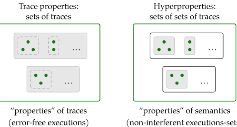
In the context of systems security, information flows play a central role. Unhandled infor-mation flows potentially leave the door open to very dangerous types of security attacks, such as code injection or sensitive information leakage. Information flows verification is based on a notion of dependency between a system’s objects, which requires specifications expressing relations between different executions of a system. Specifications of this kind, called hyperproperties, go beyond classic trace properties, defined in terms of predicate over single executions. The problem of trace properties verification is well studied, both from a theoretical as well as a practical point of view. Unfortunately, very few works deal with the verification of hyperproperties. Note that hyperproperties are not limited to information flows. Indeed, a lot of other important problems can be modeled through hyperproperties only: processes synchronization, availability requirements, integrity issues, error resistant codes check, just to name a few.
The sound verification of hyperproperties is not trivial: it is not easy to adapt classic verification methods, used for trace properties, in order to deal with hyperproperties. The added complexity derives from the fact that hyperproperties are defined over sets of sets of executions, rather than sets of executions, as happens for trace properties. In general, passing to powersets involves many problems, from a computability point of view, and this is the case also for systems verification.
In this thesis, it is explored the problem of hyperproperties verification in its theoretical and practical aspects. In particular, the aim is to extend verification methods used for trace properties to the more general case of hyperproperties. The verification is performed ex-ploiting the framework of abstract interpretation, a very general theory for approximating the behavior of discrete dynamic systems.
Apart from the general setting, the thesis focuses on sound verification methods, based on static analysis, for computer programs. As a case study – which is also a leading moti-vation – the verification of information flows specifications has been taken into account, in the form of Non-Interference and Abstract Non-Interference. The second is a weakening of the first, useful in the context where Non-Interference is a too restrictive specification.
The results of the thesis have been implemented in a prototype analyzer for (Abstract) Non-Interference which is, to the best of the author’s knowledge, the first attempt to imple-ment a sound verifier for that specification(s), based on abstract interpretation and taking into account the expressive power of hyperproperties.
Contents
Declaration of Authorship v Abstract ix List of Figures xv Preface xvii 1 Introduction 11.1 Structure of the Thesis and Contributions . . . 3
2 Mathematical Background 5 2.1 Basic Notions and Notations . . . 5
2.1.1 Relations and Functions . . . 6
2.1.2 Ordered Structures . . . 7
2.1.3 Ordinals . . . 10
2.1.4 Functions on Ordered Structures . . . 10
2.1.5 Fixpoints . . . 11
2.1.6 Galois Insertions, Closure Operators and Moore Families . . . 12
2.2 Abstract Interpretation . . . 13
2.2.1 Concrete and Abstract Objects . . . 14
2.2.1.1 Functions Abstraction . . . 15
2.2.1.2 The Optimal Case of Galois Connections . . . 15
2.2.2 Fixpoint Computations . . . 17
2.2.2.1 Fixpoint Extrapolation . . . 18
2.3 Derived Structures and Abstractions . . . 19
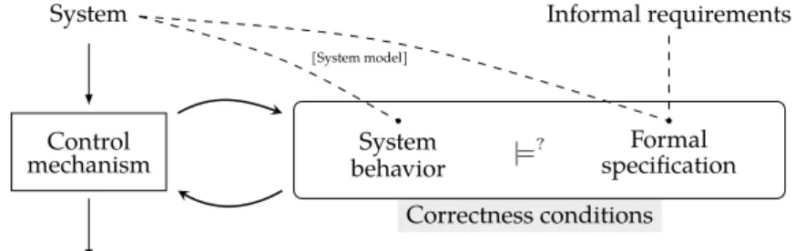
3 System Correctness 21 3.1 Correctness Condition . . . 21
3.1.1 Informal Introduction . . . 21
3.1.2 Going (a Little Bit) Formal . . . 22
3.2 Control Mechanisms: Verification vs Enforcement . . . 24
3.2.1 Analysis and Approximations . . . 25
3.3 Safety and Confidentiality Requirements . . . 26
3.3.1 Information Flow . . . 27
3.3.2 Different Flavors of Non-Interference . . . 29
3.3.2.1 Qualitative vs Quantitative Information Flow . . . 29
3.3.2.2 Declassification and Attacker’s Power . . . 30
4 Systems, Semantics and Specifications 33
4.1 Systems and Semantics . . . 33
4.1.1 Transition Systems . . . 33
4.1.1.1 System Semantics . . . 34
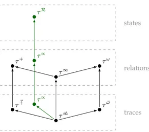
4.1.2 Hierarchy of Semantics . . . 35
4.1.2.1 Extending the Hierarchy . . . 39
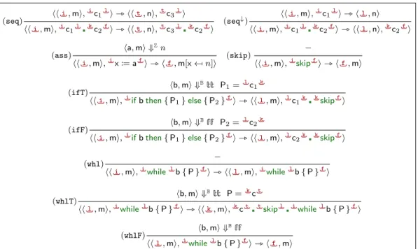
4.1.3 The Programming Language . . . 41
4.1.3.1 Program Standard Semantics . . . 42
4.2 Formalizing Specifications . . . 44
4.2.1 Hyperproperties: Introduction . . . 44
4.2.2 Hyperproperties: Topological Characterization . . . 46
4.2.2.1 Safety and Liveness Dichotomy . . . 49
4.2.2.2 Hypersafety and Hyperliveness Dichotomy . . . 50
4.2.2.3 Topologies for Trace Properties and Hyperproperties . . . 52
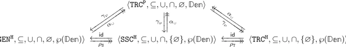
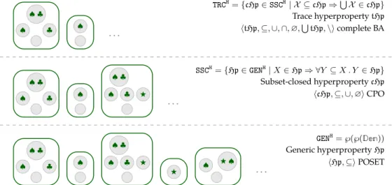
4.2.3 Hyperproperties: Algebraic Characterization . . . 55
4.2.3.1 Relations between Hyperproperties . . . 55
4.2.3.2 Trace Decomposition . . . 57
5 Classic Program Analysis 59 5.1 The Trace Properties Verification Process . . . 60
5.1.1 Computing the Maximal Trace Semantics . . . 63
5.2 Invariants Verification . . . 64
5.2.1 Computing the State Semantics . . . 64
5.2.2 Application: Non-Relational Numerical Analysis . . . 66
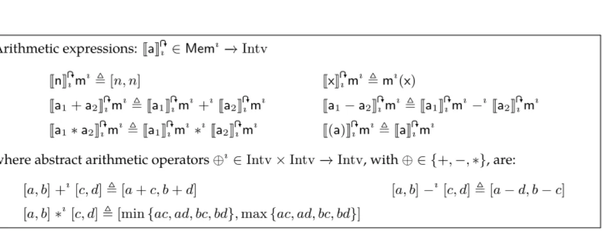
5.2.2.1 The Abstract Semantics for Intervals . . . 68
5.2.2.2 The Verification . . . 70
6 Hyper Program Analysis 73 6.1 Hyper Static Analysis . . . 73
6.1.1 The Hyperproperties Verification Issue . . . 73
6.1.2 Stronger Trace Property . . . 76
6.1.3 Equisatisfying Hyperproperty . . . 77
6.1.4 Correct Hypersemantics . . . 79
6.1.4.1 Subset-closed and Generic Hypersemantics . . . 79
6.1.4.2 Post/Pre Hypersemantics . . . 85
6.2 Hyper Abstract Domains . . . 87
6.2.1 The Compositional Nature of Hyper Abstract Domains . . . 87
6.2.1.1 Dealing with Constants Propagation . . . 89
6.2.1.2 Dealing with Intervals. . . 91
7 Bounded Subset-Closed Hyperproperties 97 7.1 Bounded Subset-Closed Hyperproperties . . . 97
7.1.1 Expressiveness . . . 99
7.2 Verification of Bounded Subset-Closed Hyperproperties . . . 100
7.2.1 Partitions-Driven Verification . . . 100
7.2.2 Not-Relational Verification . . . 102
7.3 Hypersemantics for Subset-Closed Hyperproperties . . . 106
7.3.1 On Bounded Hyperproperties . . . 110
8 Application: Verification of Information Flows 111 8.1 Abstract Hypersemantics for Abstract Non-Interference . . . 113
8.1.1 The Hypersemantics . . . 113
8.1.2 Towards Abstraction . . . 114
8.1.2.1 The Abstract Domain for Abstract Non-Interference. . . 114
8.1.3 The Parametric Abstract Semantics . . . 118
8.2 Implementation: the NonInterfer Static Analyzer . . . 122
8.2.1 Towards Abstraction . . . 123
8.2.1.1 The Abstract Domain for Non-Interference . . . 123
8.2.2 The Abstract Semantics for Non-Interference . . . 125
8.2.3 The Prototype Analyzer . . . 129
8.2.3.1 Validation . . . 129 8.2.3.2 Improving Precision . . . 130 9 Concluding Remarks 133 9.1 Related Works . . . 134 9.2 Future Directions . . . 136 A Long Proofs 137 Bibliography 167
List of Figures
2.1 Hasse diagram examples. . . 9
3.1 Control mechanism process. . . 22
3.2 Examples of flow types x y. . . 27
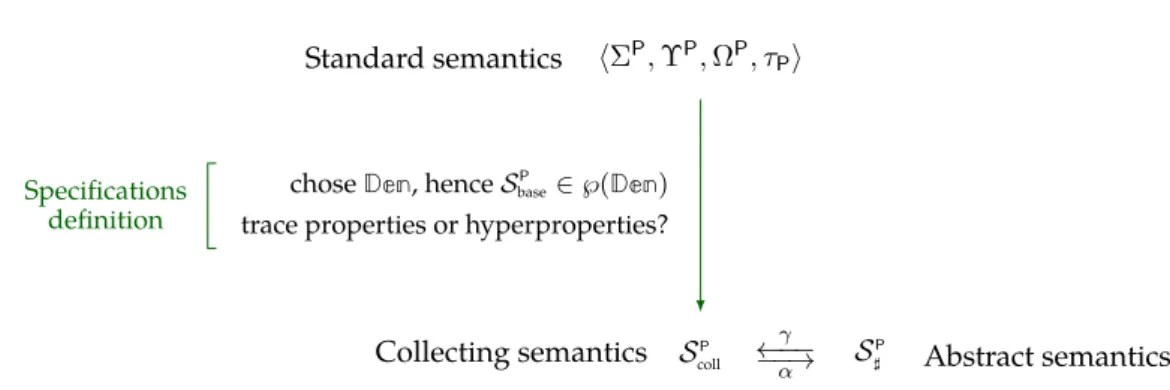
4.1 A part of the standard hierarchy of semantics, with extensions (in green). . . 40
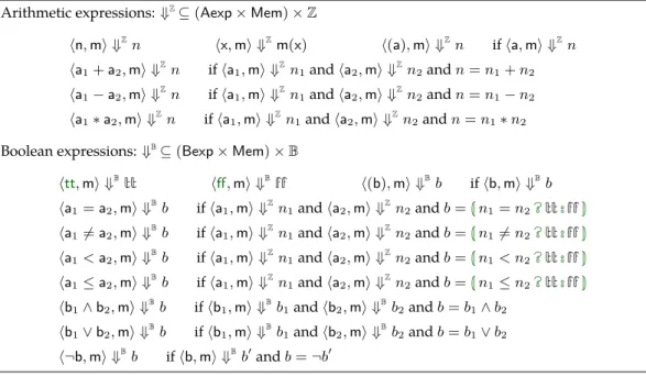
4.2 Big-step operational semantics for expressions. . . 43
4.3 Small-step operational semantics of Imp. . . 44
4.4 Trace properties and hyperproperties. . . 46
4.5 Subset-closed hyperproperties. . . 56
4.6 Relations between hyperproperties . . . 56
4.7 Hyperproperties algebraic structure. . . 57
5.1 Standard, collecting and abstract semantics. . . 60
5.2 Abstract Intervals semantics for arithmetic expressions. . . 69
6.1 Over-approximation of trace properties A and hyperpropertiesB . . . 74
6.2 Verification (abstract interpretation) of properties A and hyperpropertiesB . 75 6.3 A part of the classic hierarchy of semantics with its hyper counterpart. . . 84
6.4 Three layers abstraction. . . 89
6.5 Hyper (abstract) constants domain construction. . . 91
6.6 Abstraction and concretization of an Interval of Intervals. . . 92
7.1 Bounded subset-closed hyperproperties. . . 100
7.2 Relational and not-relational hyperproperties. . . 103
8.1 Abstract semantics for expressions. . . 119
8.2 Abstract semantics for arithmetic expressions. . . 126
8.3 Abstract semantics for boolean expressions. . . 127
Preface
The present thesis is the result of my research work, developed at the University of Verona during part of my PhD. Indeed, I spent most of my first year (out of three) working in a different research project, leading to publications [Dalla Preda and Pasqua,2016] and [Dalla Preda and Pasqua,2018], but not related to the present thesis. Nevertheless, in the remaining two years I was able to obtain some results about hyperproperties verification, namely the topic of the present thesis.
The thesis is organized in nine chapters and one appendix, containing long proofs. Chap-ter1serves as an introduction of the problem I addressed. It contains also a description of the contributions and a conceptual road-map guiding the reader through the central part of the thesis. Chapter2contains notions and mathematical notations required to fully under-stand the concepts showcased in the thesis. From Chapter3to Chapter8we have the main contributions of the thesis, interleaved with already known results and concepts. I have chosen this mixed presentation in order to make the text more easy and, hopefully, enjoy-able to read. Nevertheless, my contributions are well marked within any chapter. Finally, Chapter9concludes and discusses future research directions.
Most of the contents of this thesis have been published in international peer-reviewed conferences and they have been developed under the supervision of Isabella Mastroeni, Associate Professor at the University of Verona. In the rest of the work I adopt the academic “we” instead of “I”.
The first version of the thesis has been submitted for the reviewing process in December 15, 2018. The present text is the revised and corrected version.
Introduction
1
C
concerning systems security, a fundamental problem is how to protect the confiden-tiality or, dually, integrity of data manipulated by programs. Namely, it is important to guarantee that no confidential information can be caught by unauthorized attackers ob-serving the executions of a system. The standard way used to protect private data is accesscontrol. As the name indicates, access control verifies the system rights at entry-point and it
does not take into account the propagation of information. This is inadequate in many situ-ations, in fact the system may leak/compromise information after the access check. Instead,
information flow control tracks how information propagates through the system during
exe-cution, to make sure that it handles the information securely. Unhanded information flows potentially leave the door open to very dangerous types of attacks, such as code injection or sensitive data leakage. So, it is important to build verification mechanisms, aiming to check if systems comply with a given confidentiality/integrity specification, stating which flows of information are allowed and which are not.
The problem of information flows control is far from a solution. There are several dif-ficulties concerning information flows verification. First of all, the problem is undecidable, hence a form of approximation is mandatory. Unfortunately, also approximated verification is not easy for information flows, since they are formalized as hyperproperties. This means that they cannot be verified on single executions, since they require the comparison of mul-tiple computations: this makes hard to exploit standard verification techniques. Indeed, whilst for trace properties standard techniques can be used with an acceptable degree of ap-proximation, the verification of hyperproperties is a hard problem to solve in a sufficiently precise way. Being a hyperproperty means to be modeled as a set of sets of executions and, indeed, the extra level of sets introduces a lot of technical problems for approximation-based verification methods. Hence, in order to obtain significant results w.r.t. analysis precision, we need new verification methods which approximate sets of sets (instead of just sets) of executions, namely we need verification methods for hyperproperties.
Note that, information flows control is the leading motivation, but hyperproperties can express a lot of other useful specifications, like availability requirements, process synchro-nization problems, cryptographic protocols checks, etc. The latter, as well as information flows, cannot be expressed with classic trace properties.
The goal of the thesis is to face the problem of verifying hyperproperties, namely to de-velop a methodology which goes beyond the standard trace properties. In order to cope with this problem, we need to reason about systems semantics, namely the representations of systems executions, and hence we rely on abstract interpretation, which is a general frame-work for the sound approximation of the semantics of discrete dynamic systems.
explic-M. Pasqua
itly, to describe and formalize approximate computations in many different areas of com-puter science, from its very beginning use in formalizing (compile-time) program analysis frameworks to more recent applications in model checking, program verification, compar-ative semantics, malware detection, code obfuscation, etc. When reasoning about systems executions a key point is the degree of approximation given by the choice of the seman-tics used to represent computations. In this direction, comparative semanseman-tics consists in comparing semantics at different levels of abstraction, always by abstract interpretation. The choice of the semantics is a key point, not only for finding the desirable trade-off be-tween precision and decidability of program analysis in terms, for instance, of specifications verification, but also because not all the semantics are suitable for proving every possible specification of interest. This means that the specification to verify necessarily affects the semantics we have to choose for modeling the system to analyze.
Hyperproperties verification is a new research topic and so there are very few works about it. For this reason, we started reasoning about hyperproperties from the roots, namely from a structural point of view. In particular we characterized hyperproperties with topo-logical and algebraic approaches. With a better theoretical understanding of hyperproper-ties, we were able to tackle the problem of verification of hyperproperhyperproper-ties, which is more complex than the standard case of trace properties verification. In fact, at the “hyper level”, standard systems semantics are not useful, because they are defined at the sets of traces level. This led us to define new semantics, termed hypersemantics, computed at the same level of hyperproperties, namely at the sets of sets of executions level. In order to make the verification feasible, we still need approximation, namely simpler (i.e. approximate) versions of the systems (hyper)semantics. As already said, we perform approximation ex-ploiting the framework of abstract interpretation. Once we set the concrete semantics, in our case hypersermantics able to verify hyperproperties, we need abstract domains, in order to obtain approximate, but decidable, verification methods. The verification is performed by means of static analysis, using a decidable abstract interpretation of the hypersemantics. Clearly, classic abstract domains cannot be used for hyperproperties, hence we define some design patterns useful to generate hyperdomains, namely abstract domains for hyperproper-ties verification.
Apart from these general results, we deepen the verification problem of a restriction of subset-closed hyperproperties, i.e. bounded subset-closed hyperproperties. These hyperprop-erties are expressive enough to capture lots of interesting specifications (such as information flows) but their verification is made easier. In particular, the verification of these hyperprop-erties is bounded to a fixed input cardinality, restricting the search space for confutation. Nevertheless, also for this kind of hyperproperties, the verification has to move to the hy-perlevel. We propose a general technique for lifting the semantic operator computing the concrete systems semantics to the hyperlevel. The added value of tackling the problem from a general and formal point of view is that it allows us to discuss and prove soundness and completeness properties.
We instantiate our theoretical results to the verification of (Abstract) Non-Interference, allowing us to design a prototype verifier of Non-Interference for a toy programming lan-guage. In particular, we first design the hyperdomain denoting the hyperproperty that has to be satisfied by the semantics of non-interfering programs, i.e. the values of public vari-ables must be always the same single value. Once we fix the domain of the abstract ob-servable hyperproperty we define the abstract hypersemantics computing the executions
Chapter 1. Introduction M. Pasqua
of a program on the hyperdomain, exactly as it happens in classic static analysis, but with the only difference that we are abstracting an hypersemantics into an hyperdomain. To the best of our knowledge, this is the first attempt to provide a sound analyzer/verifier of Non-Interference exploiting the expressiveness of hyperproperties. Finally, in order to test the feasibility of the proposed approach we have implemented a prototype (called nonInterfer) of the designed verifier. This prototype exhibits a good trade-off between verification speed and precision.
1.1
Structure of the Thesis and Contributions
Apart from this chapter, Chapter2introduces the basic mathematical concepts needed to understand the work and the notations adopted in the rest of the thesis. At the end of the chapter we can find a general introduction to abstract interpretation, which is the main framework we will use. The central part of the thesis comprises chapters from3to8.
In Chapter3we introduce the problem of systems correctness which, basically, requires the definition of a (mathematical) model of the system and a (mathematical) description of a specification. Furthermore, concepts as verification, enforcement, systems analysis and approximations are described. Finally, we list some examples of common systems specifi-cations and, in particular, we focus on information flows.
In Chapter 4 we introduce in detail the system model we have chosen, i.e. transition systems, and how to retrieve the behavior, i.e. the semantics, associated to a system. We do the same for specifications, namely we introduce hyperproperties. In Section4.2.2we investigate these latter from a theoretical point of view, giving a topological and algebraic characterization of hyperproperties. The topological characterization has been published in [Pasqua and Mastroeni, 2017]. At the end of Section4.1.1we describe a very simple programming language Imp, which will be used in the rest of the thesis. Indeed, starting from Chapter5, the systems we take into account are programs written in Imp.
Chapter5 aims to make the reader familiar with classic program verification of trace properties. We perform verification by means of analysis, formalized as an abstract inter-pretation of the concrete program semantics. In particular we build step by step a very simple numerical analysis for programs in Imp. This latter will be taken as a comparison for the case of hyperproperties verification.
Then we go at the hyperlevel. In Chapter6.1we deal with the problem of program ver-ification of hyperproperties. Unfortunately, it is not easy to adapt classic static analysis for trace properties, to the more general hyperproperties. In this chapter we highlight the prob-lems concerning hyperproperties verification and some possible solutions. Furthermore, we show how to define, in a constructive way, hypersemantics, i.e. program semantics com-puting at the level of sets of sets. Every abstract interpretation needs an abstract domain, in order to perform approximate verification. Hence, in Section6.2, we take into account the problem of defining hyperdomains, namely abstract domains fro hyperproperties. Most of the results presented in this chapter have been published in [Mastroeni and Pasqua,2017] and, partially, in [Mastroeni and Pasqua,2018].
In Chapter7 we focus on particular hyperproperties, the bounded subset-closed one, which exhibit a good trade-off between expressiveness and verification feasibility. Indeed, they could express, among other specifications, information flows and their verification can
M. Pasqua 1.1. Structure of the Thesis and Contributions
be simplified significantly. In particular, we show how to adapt the existing classic static analyses, by lifting the semantic operator used to define the concrete semantics. Some parts of this chapter have been published in [Mastroeni and Pasqua,2018].
Chapter 8 concludes the contributions of the thesis, giving an applicative example of our theoretical findings. In particular, exploiting the result of Chapter7we develop a (para-metric) abstract semantics for Abstract Interference and an abstract semantics for Non-Interference. These are formalizations of information flows specifications, hence we build a feasible and sound verification mechanism for information flows. The abstract seman-tics for Non-Interference has been implemented in a prototype verifier for Imp programs, called nonInterfer. The part of this chapter concerning Non-Interference has been published in [Mastroeni and Pasqua,2019].
Finally, in Chapter 9we discuss related works, the possible future research directions and the concluding remarks.
Publications. Most of the results presented in the thesis have been already published in: [Mastroeni and Pasqua,2017] Isabella Mastroeni and Michele Pasqua (2017). “Hyper-hierarchy of Semantics - A Formal Framework for Hyperproperties Verification”. In: Static
Analysis - 24thInternational Symposium, (SAS 2017), New York City, USA, August 30 –
Septem-ber 1, 2017, Proceedings, pp. 232–252. doi: 10.1007/978- 3- 319- 66706- 5_12. url: https: //doi.org/10.1007/978-3-319-66706-5_12
[Pasqua and Mastroeni, 2017] Michele Pasqua and Isabella Mastroeni (2017). “On topologies for (hyper)properties”. In: 18th Italian Conference on Theoretical Computer Science (ICTCS 2017), Naples, Italy, September 26 – 28, 2017, Proceedings, pp. 1–12. url: http://ceur-ws.org/Vol-1949/ICTCSpaper13.pdf
[Mastroeni and Pasqua,2018] Isabella Mastroeni and Michele Pasqua (2018). “Verify-ing Bounded Subset-Closed Hyperproperties”. In: Static Analysis. Ed. by Andreas Podelski. Cham: Springer International Publishing, pp. 263–283. isbn: 978-3-319-99725-4
[Mastroeni and Pasqua,2019] Isabella Mastroeni and Michele Pasqua (2019). “Stati-cally Analyzing Information Flows – An Abstract Interpretation-based Hyperanalysis for Non-Interference”. In: Proceedings of the 34rd Annual ACM Symposium on Applied Computing. SAC ’19. Limassol, Cyprus: ACM, pp. 2215–2223. isbn: 978-1-4503-5933-7. doi: 10.1145/ 3297280.3297498
Mathematical Background
2
T
his chapter introduces mathematical notations, basic notions and existing results that are at the foundation of our work and will serve in subsequent chapters. Then, in the last section, we provide an overview of abstract interpretation, which is the principal theory we use in our work.2.1
Basic Notions and Notations
We recall now some basic notations of set theory. A set is a (not proper) class of distinct and unordered objects. When an object x is a member, or an element, of the set X we write x ∈ X, we write x /∈ X otherwise. We represent extensionally a (finite) set, the elements of which are x1, x2, . . . xn, with the notation {x1, x2, . . . xn}. Dually, we represent intensionally a (sub)set (of a set U ), the elements of which fulfill a predicate φ, with the notation {x ∈ U | φ(x)}. When U is clear from the context, we often omit it for brevity. The predicate φis specified by a first-order formula possibly containing the classic logical operators: ∧ (conjunction), ∨ (disjunction), ¬ (negation), ⇒ (implication), ⇔ (logical equivalence), ∀ (universal quantification), ∃ (existential quantification). The empty set is denoted by ∅ and the cardinality of a set X is denoted by |X|.
A set Y is a subset of a set X, written Y ⊆ X, if and only if every element of Y is in X. The empty set is a subset of every set. The set of all subsets of a set X, denoted ℘(X), is defined as ℘(X) , {Y | Y ⊆ X}. Here the symbol , stands for “is defined as”, in contrast to the symbol = which stands for “is the same as”. The union of two sets X and Y , written X ∪ Y , is the set of elements belonging to X or Y , namely: X ∪ Y , {x | z ∈ X ∨ z ∈ Y }. More generally, the union of a family of sets X , denoted byS X , is S X , SX∈XX = {x | ∃X ∈ X . x ∈ X}. Similarly, the intersection of two sets X and Y , written X ∩ Y , is the set of elements belonging to X and Y , namely: X ∩ Y , {x | z ∈ X ∧ z ∈ Y }. More generally, the intersection of a family of sets X , denoted byT X , is T X , TX∈XX = {x | ∀X ∈ X . x ∈ X}. The set-difference between set X and one of its subsets Y , denoted by X \ Y , is the set of all elements of X which are not elements of Y , namely X \ Y , {z | z ∈ X ∧ z /∈ Y }. Given a set X, a set P ⊆ ℘(X) is a partition (of X) when P 6= ∅,S
P ∈PP = Xand for every P1, P2∈ P either P1= P2or P1∩ P2= ∅.
The cartesian product of two sets X and Y , written X × Y , is the set of all pairs where the first component is in X and the second component is in Y , namely X × Y , {hx, yi | x ∈ X ∧ y ∈ Y }. The cartesian product can be extended to n-tuples, with n > 2: X1× X2× . . . Xn, {hx1, x2, . . . xni | ∀i ∈ {1, 2, . . . n} . xi ∈ Xi}. We write Xnin order to denoted the n-times cartesian product of X with itself.
M. Pasqua 2.1. Basic Notions and Notations
set of natural numbers is denoted by N and the set of integer numbers is denoted by Z. A numeric (integer) interval [n, m] is the set of all integer numbers between n and m, called bounds, namely [n, m] , {x ∈ Z | n ≤ x ∧ x ≤ m}. When the left bound is not in the set we use ‘]’ in place of ‘[’, i.e. ]n, m] , [n, m] \ {n} (and similarly for the right bound).
Finally, we will often use, in order to shorten the notation, the inline conditional con-struct(cond?doTrue:doFalse), borrowed from programming languages like C and Java. The meaning is that the construct is replaced by the term doTrue if the condition cond is satisfied and by the term doFalse otherwise.
2.1.1
Relations and Functions
A relation R between sets X1, X2, . . . Xn, for n ∈ N, is a subset of the cartesian product X1× X2× . . . Xn. The elements xi, such that xi ∈ Xifor every i ∈ [1, n], are in relation R when hx1, x2, . . . xni ∈ R ⊆ X1× X2× . . . Xn. A relation R is binary when n = 2, namely R ⊆ X1× X2. We often write x1 R x2for hx1, x2i ∈ R and x1 6R x2 for hx1, x2i /∈ R. The composition of a relation R1 ⊆ X × Y with a relation R2 ⊆ Y × Z is the relation R2◦ R1⊆ X × Z defined as R2◦ R1, {hx, zi | ∃y ∈ Y . x R1y ∧ y R2z}.
A binary relation R on a set X is a subset of X × X and could have some important properties: reflexivity ∀x ∈ X . x R x irreflexivity ∀x ∈ X . x 6R x symmetry ∀x, y ∈ X . x R y ⇒ y R x antisymmetry ∀x, y ∈ X . x R y ∧ y R x ⇒ x = y transitivity ∀x, y, z ∈ X . x R y ∧ y R z ⇒ x R z totality ∀x, y ∈ X . x R y ∨ y R x
A binary relation is termed equivalence if it is reflexive, symmetric, and transitive. In a set with an equivalence relation, we consider, for each x ∈ X, the subset of X containing all the elements y ∈ X such that xRy. This set is called equivalence class of x (in X, through R) and usually it is denoted by [x]R. An equivalence relation induces a partition of the set on which it is defined, and the elements of the partition are its equivalence classes.
A binary relation is a preorder if it is reflexive and transitive. A partial order is an antisym-metric preorder. A partial order which is total is called a total order (or linear order). Partial or a total orders are strict if they are irreflexive instead of reflexive. Note that, for strict or-ders, the antisymmetry requirement is useless: xRy and yRy cannot both hold since, by transitivity, this would imply xRx, which cannot hold by irreflexivity.
A function f from the set X, called domain, to the set Y , called co-domain, is a relation f ⊆ X × Y such that:
• {x ∈ X | hx, yi ∈ f } = X
• if hx, yi ∈ f and hx, y0i ∈ f then y = y0
Chapter 2. Mathematical Background M. Pasqua
This means that a function maps every element of X to one, and only one, element of Y . The element of y in relation with x ∈ X is said its image and it is usually written y = f (x). The set of all functions from X to Y is denoted by X −→ Y . When we need to describe functions extensionally, we will use the following notation: [x17→ y1x27→ y2 . . . xn7→ yn]denotes the function {hx1, y1i, hx2, y2i, . . . hxn, yni}. We will often use the lambda notation to denote a function: λx . f (x). The composition of a function f ∈ X −→ Y with a function g ∈ Y −→ Z is a function g ◦ f ∈ X −→ Z such that: ∀x ∈ X . g ◦ f (x) = g(f (x)).
A function f ∈ X −→ Y could have some important properties: injectivity ∀x, x0∈ X . f (x) = f (x0) ⇒ x = x0
surjectivity ∀y ∈ Y ∃x ∈ X . f (x) = y
An injective function is also called one-to-one, whilst a surjective function is also called onto. A bijection (or isomorphism) is an injective and surjective function. The inverse of a bijective function f ∈ X −→ Y is the bijective function f−1
, {hy, xi | hx, yi ∈ f }. The direct image (sometimes called additive lift) of f ∈ X −→ Y is the the function ˆf ∈ ℘(X) −→ ℘(Y ) mapping a set Z ⊆ X to the set of images of elements in Z, namely: ˆf (Z) , {f (z) | z ∈ Z}. Sometimes, we will abuse notation denoting with f (Z) the direct image of f on Z.
A partial function f from the set X the set Y is a relation f ⊆ X × Y such that: • if hx, yi ∈ f and hx, y0i ∈ f then y = y0
Technically, the term partial function is improper, since partial functions are not functions. Partial functions model the fact that for some elements of the domain the function is not defined. The set of all partial functions from X to Y is denoted by X ,−→ Y . As for relations, we can define functions with more than one argument: f ∈ X1× X2× . . . Xn−→ Y . Usually, the notation f (hx1, x2, . . . xni) = y is replaced with f (x1, x2, . . . xn) = y.
In the rest of the thesis, we will use very often the pointwise extension of relations and functions, as described in the following definition.
Definition 1(Pointwise Extension). Let X, Y, Z be arbitrary sets.
• The pointwise extension of a relation ≤ ⊆ Y × Y is a relation ˙≤X⊆ (X −→ Y ) × (X −→ Y )defined as: ˙≤X, {hf, gi | ∀x ∈ X . f (x) ≤ g(x)}.
• The pointwise extension of a function α ∈ Y −→ Z is a function ˙αX ∈ (X −→ Y ) −→ (X −→ Z) defined as: ˙αX , λf . λx . α(f (x)).
• The pointwise extension of an operatorW ∈ ℘(Y ) −→ Y is an operator ˙W
X ∈ ℘(X −→ Y ) −→ (X −→ Y ) defined as: ˙W
XW , λx .W{f (x) | f ∈ W }. Usually, the subscripts are omitted when X is clear from the context.
2.1.2
Ordered Structures
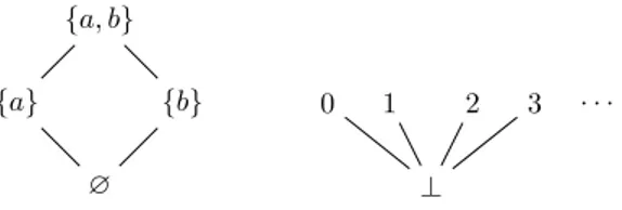
A set X with a partial order ≤, denoted hX, ≤i, is called partially ordered set or, more con-cisely, POSET. If the relation ≤ is just a preorder, then hX, ≤i is called preordered set or, PROSET. Finite partially ordered sets can be drawn as line diagrams, called Hasse diagrams (Figure2.1, on the left). We can draw also an infinite POSET by showing a finite part which
M. Pasqua 2.1. Basic Notions and Notations
illustrates the building principle (Figure2.1, on the right). In a Hasse diagram, each ele-ment x ∈ X is uniquely represented by a node of the diagram, and there is an edge from a node x to a node y if y covers x, namely, x ≤ y and there exists no z ∈ X such that x ≤ z ∧ z ≤ y. Hasse diagrams are usually drawn placing the elements higher than the elements they cover.
Let hX, ≤i be a POSET and let Y ⊆ X. We say that u ∈ X is an upper bound of Y if ∀y ∈ Y . y ≤ u; u is said maximal if it also belongs to Y . If the set of upper bounds (of Y ) has the smallest element, then we call this latter least upper bound (or lub; join; supremum) of Y , denotedW Y (or sup Y ). If the lub belongs to Y then it is said maximum (or top) and it is usually denoted by > (or max Y ). Dually, we say that l ∈ X is a lower bound of Y if ∀y ∈ Y . l ≤ y; l is said minimal if it also belongs to Y . If the set of lower bounds (of Y ) has the biggest element, then we call this latter greatest lower bound (or glb; meet; infimum) of Y , denotedV Y (or inf Y ). If the glb belongs to Y then it is said minimum (or bottom) and it is usually denoted by ⊥ (or min Y ). Note that maximum, minimum, supremum and infimum, when they exist, are unique. In general, we denote by x ∨ y and x ∧ y, the elements W{x, y} and V{x, y}, respectively.
A PROSET hX, ≤i is called directed if every pair of elements x, y ∈ X has an upper bound in X. This is equivalent to say that every non-empty finite subset of X has an upper bound. Since a POSET is, in particular a PROSET, the definition of directed POSET is immediate. A
(directed) complete partial order or, more concisely DCPO, is a partially ordered set in which
every non-empty directed subset has a least upper bound. If a DCPO has a minimum, it is called pointed.
A subset of a partially ordered set is called a chain, when the partial order is total if restricted to the elements of the chain only. Note that every chain is a directed POSET. A partially ordered set is chain-complete when every chain, including the empty chain, has a least upper bound. The fact that the lub for the empty chain ∅ exists implies that the POSET has a minimum elementW
∅.
An important result in order theory is that a partially ordered set is a pointed DCPO if and only if it is chain-complete, but it is provable only if we assume the axiom of choice (a proof can be found in [Markowsky,1976]). Due to this equivalence, in the following we use the term complete partial order or, more concisely, CPO to refer a pointed DCPO or a chain-complete POSET. We denote a CPO with the tuple hX, ≤, ∨, ⊥i, where ∨ is the partial least upper bound operator (see Definition2) and ⊥ is the minimum.
A POSET hX, ≤i satisfies the ascending chain condition (ACC in short) if and only if any infinite increasing chain x0 ≤ x1 ≤ . . . of elements of X is not strictly increasing, namely: ∃k ∈ N such that ∀j > k . xk = xj. Dually, it satisfies the descending chain condition (DCC in short) if and only if any infinite decreasing chain . . . ≤ x1 ≤ x0of elements of X is not strictly decreasing, namely: ∃k ∈ N such that ∀j > k . xk = xj. Note that if a POSET has minimum and it is ACC, then it is a CPO.
A POSET hX, ≤i is a join-semilattice (or ∨-semilattice) if every pair of elements x, y ∈ X has a least upper bound. This is equivalent to say that every non-empty finite subset of X has a least upper bound. A join-semilattice is said bounded if it has minimum, namely the least upper bound of ∅, and it is said complete if it has a least upper bound for every subset of X. Dually, it is a meet-semilattice (or ∧-semilattice) if every pair of elements x, y ∈ X has greatest lower bound. This is equivalent to say that every non-empty finite subset of X has greatest lower bound. A meet-semilattice is said to be bounded if it has maximum,
Chapter 2. Mathematical Background M. Pasqua {a, b} {b} {a} ∅ . . . 3 2 1 0 ⊥
Figure 2.1: Hasse diagram examples.
namely the greatest lower bound of ∅, and it is said complete if it has a least upper bound for every subset of X. A lattice is a join-semilattice which is also a meet-semilattice. In a similar way, we obtain the notions of bounded and complete lattice. We denote a complete lattice with the tuple hX, ≤, ∨, ∧, ⊥, >i, where ∨ is the (total) least upper bound operator, ∧ is the (total) greatest lower bound operator, ⊥ is the minimum and > is the maximum.
So we can distinguish the ordered structures, depending on the subsets which have least upper bound (or, dually, on the subsets which have greatest lower bound). In order to be clear, we define the following operator.
Definition 2. Let hP, ≤i be a POSET, then a partial least upper bound operator ∨ ∈ ℘(P ) ,−→ P is a partial function such that, for every X ∈ ℘(X) if ∨(X ) is defined then the least upper bound of X , i.e.W X , exists and ∨(X ) = W X .
So we can discriminate the various ordered structures introduced so far by looking when this operator is defined, as we can see in the following table.
∨(X ) is, at least, defined when
POSET X is a singleton
POSET with minimum X is a singleton or X = ∅
DCPO X is directed
pointed DCPO X is directed or X = ∅
chain-complete POSET X is a, possibly empty, chain join-semilattice X is a non-empty finite set bounded join-semilattice X is a finite set complete join-semilattice X is a set
It is clear that the partial least upper bound operator is a total function if and only if it is defined over a complete lattice. We abuse notation denoting in the same way the least upper boundW X of a set X and the partial least upper bound operator ∨(X ) applied to X .
Let hX, ≤i be a POSET with minimum ⊥ and maximum >. For each x ∈ X we say that y ∈ X is the complement of x if x ∧ y = ⊥ and x ∨ y = >. A lattice where every element has a complement is called complemented. The complement of x is denoted as ¬x. A lattice such that for all x, y, z ∈ X we have x ∧ (y ∨ z) = (x ∧ y) ∨ (x ∧ z) and x ∨ (x ∧ z) = (x∨y)∧(x∨z)is called distributive. A boolean algebra or, more concisely BA, is a complemented and distributive lattice. If the lattice is complete then the boolean algebra is said complete as well. We denote a complete BA with the tuple hX, ≤, ∨, ∧, ⊥, >, ¬i, where ∨, ∧, ⊥, > have the same meaning as in the case of a complete lattice and ¬ is the (total) complement operator.
M. Pasqua 2.1. Basic Notions and Notations
2.1.3
Ordinals
A set equipped with a total order is said totally ordered (or linearly ordered; simply ordered). Note that a chain is totally ordered. A binary relation R over a set X is well-founded when every non-empty subset of X has a least element with respect to R. A well-founded total order is called a well-order (or well-ordering). A well-ordered set hW, ≤i is a set W equipped with a well-ordering ≤.
Every well-ordered set is associated with an order type. Two well-ordered sets hW1, ≤2i and hW2, ≤2i have the same order type if and only if they are order-isomorphic, that is, if there exists a bijective function f ∈ W1−→ W2such that, for all elements x, y ∈ W1we have: x ≤1y ⇔ f (x) ≤2f (y). An ordinal is the order type of a well-ordered set and it represents all well-ordered sets which are order-isomorphic to it. In fact, a well-ordered set hW, ≤i, with order type β, is order-isomorphic to the well-ordered set of all ordinals strictly smaller than the ordinal β itself, namely it is order-isomorphic to the well-ordered set {w ∈ W | w < β}. Here < is the strict version of the relation ≤. This property permits to define each ordinal as the well-ordered set of all ordinals that precede it, namely:
0 , ∅ is the smallest ordinal
β + 1 , β ∪ {β} is a successor ordinal
Thus, the first successor ordinal is 1 , {0} = {∅}. The next is 2 , {0, 1} = {∅, {∅}}. Continuing in this manner, we obtain all natural numbers, that is, all finite ordinals. A limit ordinal is an ordinal number which is neither 0 nor a successor ordinal, namely λ is a limit ordinal when ∀β < λ . β + 1 < λ. The set N of all natural numbers, denoted as an ordinal by ω, is the first limit ordinal and the first transfinite ordinal (or infinite ordinal). Using ordinals we can use a technique, generalizing the classic induction on naturals, to prove or define properties of uncountable sets.
Definition 3(Transfinite Induction). A property φ holds for each ordinal β if: base case φ(0)holds
successor case for each successor ordinal β + 1: φ(β) holds implies φ(β + 1) holds limit case for each limit ordinal λ: ∀β < λ, φ(β) holds implies φ(λ) holds
The classic induction principle works only for denumerable sets and it coincides with the transfinite induction of Definition3where we do not have the limit case and where the successor ordinals we take into account are only those strictly smaller that ω.
2.1.4
Functions on Ordered Structures
Let hD, ≤i and hD], ≤]i be two POSET. A function f ∈ D −→ D]is said to be monotonic (or
monotone; order preserving) when, for each x, y ∈ D, x ≤ y ⇒ f (x) ≤] f (y). It is Scott-continuous when it preserves existing least upper bounds of directed subsets, that is, for
di-rected sets Z ⊆ D, ifW Z exists then W]
{f (x) | x ∈ Z} exists and f (W Z) = W]
{f (x) | x ∈ Z}. The definition can be equivalently given using (lub of) non-empty chains in place of directed subsets. Dually, it is Scott-co-continuous when it preserves existing greatest lower bounds of
10 10
Chapter 2. Mathematical Background M. Pasqua
co-directed1subsets, that is, ifV Z exists, for a co-directed set Z ⊆ D, then V]
{f (x) | x ∈ Z} exists and f (V Z) = V]
{f (x) | x ∈ Z}. A function f is said (completely) additive (or com-plete join-morphism) if it preserves existing least upper bounds of arbitrary non-empty sets. Dually, f is said (completely) multiplicative (or complete meet-morphism; co-additive) if it preserves existing greatest lower bounds of arbitrary non-empty sets. Finally, f is said strict if it preserves bottom elements, namely, whenever bottom elements ⊥ ∈ D and ⊥] ∈ D]
exist, then f (⊥) = ⊥].
Definition 4(Iteratable Function). Given a POSET hX, ≤i, with partial least upper bound operator ∨ ∈ ℘(X) ,−→ X, we say that a monotone function f ∈ X −→ X is ∨-iteratable on x ∈ Xwhen the transfinite iterates of f from x, defined as,
fλ, x if λ = 0 f (fβ) if λ = β + 1 W β<λfβ if λ is a limit ordinal are well-defined.
2.1.5
Fixpoints
Given a partially ordered set hX, ≤i and a function f ∈ X −→ X, a fixpoint of f is an element x ∈ X such that f (x) = x. An element x ∈ X such that x ≤ f (x) is called a pre-fixpoint while, dually, a post-fixpoint is an element x ∈ X such that f (x) ≤ x. The ≤-least fixpoint of f , written lfp≤
f, is a fixpoint of f such that, for every fixpoint x ∈ X of f , lfp≤
f ≤ x. We write lfp≤
xf for the ≤-least fixpoint of f which is greater than, or equal to, an element
x ∈ P. Dually, we define the ≤-greatest fixpoint of f , denoted by gfp≤
f, and the ≤-greatest fixpoint of f smaller than, or equal to, x ∈ X, denoted by gfp≤
xf.
It is interesting, and useful, to know whether a function admits fixpoints, in particular the least and of the greatest one. For this reason, we recall some important fixpoint theo-rems.
Theorem 1(Knaster-Tarski Fixpoint Theorem). Let hL, ≤, ∨, ∧, ⊥, >i be a complete lattice and f ∈ L −→ L monotonic. The set of fixpoints of f is a complete lattice.
As a corollary of the theorem, we have that f has a ≤-least fixpoint lfp≤
f = V{x ∈ P | f (x) ≤ x}and a ≤-greatest fixpoint gfp≤f =
W{x ∈ P | x ≤ f (x)}. These characteri-zations guarantee that fixpoints exist but do not gives us any hint on how we can compute such fixpoints. Another fixpoints characterization, which is constructive, is the following. Theorem 2(Kleene Fixpoint Theorem). Let hD, ≤, ∨, ⊥i be a CPO and f ∈ D −→ D
Scott-continuous. Then, f has a ≤-least fixpoint which is the least upper bound of the increasing chain
⊥ ≤ f (⊥) ≤ f2(⊥) ≤ . . . namely: lfp≤ ⊥f = W n<ωf n(⊥) =W{fn (⊥) | n ∈ N}.
M. Pasqua 2.1. Basic Notions and Notations
This ensures that the fixpoint is reached in, at most, a denumerable number of steps. Note that the number of steps is finite when the the CPO satisfies the ascending chain con-dition. A dual result holds for the greatest fixpoint case.
Having a continuous function is a strong assumption, hence we show now another fix-points constructive characterization, which relaxes the continuity condition, but requires a possibly transfinite iteration.
Theorem 3(Cousot Fixpoint Theorem). Let hD, ≤i be a DCPO (not necessarily pointed), f ∈ D −→ D monotonic and x ∈ D a pre-fixpoint. Then, the iteration sequence:
fλ, x if λ = 0 f (fβ) if λ = β + 1 W β<λf β if λ is a limit ordinal
converges towards the ≤-least fixpoint lfp≤ xf.
The theorem basically says that f is ∨-iteratable on x, with respect to the partial least upper bound operator ∨ ∈ ℘(D) ,−→ D, and its least fixpoint greater than x is given by the transfinite iterates of f from x.
2.1.6
Galois Insertions, Closure Operators and Moore Families
Given a POSET hX, ≤i, a monotone function ρ ∈ X −→ X is an upper closure operator (or uco) if it satisfies the following conditions:
extensivity ∀x ∈ X . x ≤ ρ(x)
idempotence ∀x ∈ X . ρ(ρ(x)) = ρ(x)
Vice versa, if ρ is reductive, namely ∀x ∈ X . ρ(x) ≤ x, and idempotent then it is called lower closure operator (or lco). An upper closure operator is fully identifiable with the sets of its fixpoints, denoted as ρ(X) = {x ∈ X | ρ(x) = x}. We denote the set of all closure operators of X as uco(X).
Let hD, ≤i and hD], ≤]i be two POSETs. Consider two monotone functions α ∈ D −→ D]
and γ ∈ D]−→ D. We say that (D, α, γ, D])is a Galois connection, shortly GC, when
∀x ∈ D ∀x]∈ D]. x ≤ γ(x]) ⇔ α(x) ≤]x]
In this case we write:
hD, ≤i −−→←−−αγ hD]
, ≤]
i
Here, α and γ are said to be adjoint functions2, where α is the left (or upper) adjoint and γ is
the right (or lower) adjoint. An important feature of adjoint functions is that each adjoint can be uniquely determined by using the other one in the following way:
α = γ+, λx .^{x]∈ D]| x ≤ γ(x])}
γ = α−, λx]
._{x ∈ D | α(x) ≤]
x]
}
2The term adjoint is borrowed from category theory, indeed α and γ are basically adjoint (covariant) functors between the categories induced by the underlining POSETs.
12 12
Chapter 2. Mathematical Background M. Pasqua
This is tantamount to say that α is additive, i.e. α(W Y ) = W]
{α(x) | x ∈ Y }, and γ is co-additive, i.e. γ(V Y ) = V]
{γ(x]) | x]∈ Y }. Galois connections have also other nice algebraic
properties:
• γ ◦ α is extensive and idempotent • α ◦ γ is reductive and idempotent • γ ◦ α ◦ γ = γ and α ◦ γ ◦ α = α
When α ◦ γ is the identity function id = λx]. x]on D], we say that (D, α, γ, D])is a Galois insertion, shortly GI. In this case we write:
hD, ≤i −− →←−−−−→α γ
hD], ≤]i
In a Galois insertion we have that α is surjective and γ is injective. We can always obtain a Galois insertion starting from a Galois connection. This process is called reduction and it consists in collecting together all the elements x]∈ D]having the same image under γ.
When we also have that γ ◦ α is the identity function id = λx . x on D, we say that (D, α, γ, D])is a Galois isomorphism. In this case we write:
hD, ≤i −− →←−−−←−→α γ
hD], ≤]i
It is called Galois ismorphism because α and γ are bijective functions.
Let hX, ≤i be a POSET with maximum >. Then Y ⊆ X is a Moore family of X when for every Z ⊆ Y we have thatV Z exists and, in particular, V Z ∈ Y . This implies that V
∅ = > ∈ Y . A Moore family is hence closed under meet. The Moore closure of a set Y ⊆ X is defined as M(Y ) , {V Z | Z ⊆ Y }, namely M(Y ) is the smallest (w.r.t. set inclusion) subset of X which contains Y and which is a Moore family of X.
An important fact is that there is a strong link between upper closure operators, Galois insertion and Moore families. Indeed, for every Galois insertion (D, α, γ, D]), we have that
γ ◦ αis an upper closure operator of D. Dually, given a ρ ∈ uco(D) and an isomorphism ι ∈ ρ(D) −→ D]we have that (D, ι ◦ ρ, ι−1, D])is a Galois insertion. Note that if we chose
D] = ρ(D), then the isomorphism ι is just the identity function id = λx . x and the Galois
insertion is (D, ρ, id, ρ(D)). The set of fixpoints of an upper closure operator in uco(X) is a Moore family of X. Hence, we have that D]in a Galois insertion (D, α, γ, D])is isomorphic
to a Moore family of D.
Finally, note that Moore families, and hence the set of fixpoints of upper closure opera-tors, are closed under meet but not necessarily under join.
2.2
Abstract Interpretation
The prominent application of abstract interpretation is static analysis, where it is used for the definition of abstract semantics of programs. In this setting, the concrete semantic of a program, namely its “meaning”, is a representation of all its possible behaviors by means of a mathematical object (usually a set). This latter is, in general, not computable: it is not possible to represent and to compute all possible behaviors of any program in all its possi-ble execution environments. Clearly all non trivial properties of the concrete semantics of
M. Pasqua 2.2. Abstract Interpretation
a program are undecidable: it is not possible to answer any question about the behaviors of every program. For this reason abstract interpretation is born, as a theory for the sound approximation of the semantics of discrete dynamic systems. The approximation consists in the observation of the semantics at a specified level of abstraction, focusing only on the important aspects of the computation. In this setting abstract interpretation permits to cal-culate a (computable) abstract semantics of the system, parametrized on the properties of interest. The approximation is sound by design, in the sense that what holds in the abstract holds also in the concrete (no false negatives).
Remark. The choice of the concrete semantics, and consequently the abstract semantics, is
relative to the goal of the analysis. Indeed, it is possible that an abstract semantics could be the concrete semantics w.r.t. another one. Abstract interpretation is a theory for relating a concrete and an abstract semantics, hence the focus is in this relation, not in the semantics themselves.
Abstract interpretation is not limited to static analysis. Indeed, it is a theoretical frame-work to reason about computing systems but, at the same time, it offers a constructive methodology to build formal algorithms that manipulate them. So it is not surprising that abstract interpretation is applied in a lot of fields of computer science: static analysis [Cousot and Cousot,1977], type inference [Cousot,1997], model checking [Clarke, Grum-berg, and Long, 1994], comparative semantics [Comini, Levi, and Meo, 2001], program transformation [Cousot and Cousot,2002], automatic deduction [Plaisted,1981], database queries optimization [Helm, Marriott, and Odersky, 1995], cryptography [Adi and Deb-babi, 2003], quantum computing [Perdrix,2008], etc. In the following we introduce the basic concepts of abstract interpretation, in a general setting.
2.2.1
Concrete and Abstract Objects
In the most general sense, abstract interpretation is a theory for the approximation of math-ematical objects, whatever these objects refer to. Indeed, abstract interpretation is not fo-cused on the meaning of these objects but in the relation between concrete and abstract, i.e. approximated, elements. The goal of abstract interpretation is to give the formal means for relating mathematical objects at different levels of abstraction, potentially transferring the computations from the concrete level to the abstract one.
The concrete objects domain O describes the elements of interest. For instance, sets of numbers, functions, collecting semantics of programs, etc. The goal of abstract interpre-tation is to approximate concrete objects with abstract ones, chosen in an abstract objects domain O]. In other words, the intention of an abstract interpretation is to find an abstract
object A in the abstract domain O]which is a correct approximation of the concrete object
C ∈ O. Concrete and abstract objects came with two relations stating the relative precision between elements: more precise elements (concrete or abstract) carry more information. This means that hO, 4i and hO]
, 4]i are POSET and C ∈ O is more precise than C0 ∈ O if
and only if C 4 C0. Analogously, A ∈ O]is more precise than A0 ∈ O]
if and only if A 4]A0.
Usually, 4 is called approximation order and 4]is called abstract approximation order.
Cor-rectness, more often said soundness, is given by a correctness relation, stating which are the correct approximations of a concrete object. This relation can be defined in a lot of ways, de-pending on the algebraic properties that concrete and abstract domains have (see [Cousot and Cousot,1992] for a detailed explanation). In the following, we assume that the
sound-14 14
Chapter 2. Mathematical Background M. Pasqua
ness relation is given in terms of either a monotonic abstraction function α ∈ O −→ O]or
a monotonic concretization function γ ∈ O] −→ O. This means that α(C) ∈ O]is a correct
approximation of C ∈ O, or similarly, that A ∈ O]is a correct approximation of γ(A) ∈ O.
The domains are called approximation domains, since they are useful for comparing objects, w.r.t. their precision.
The monotonicity of the abstraction, or the concretization, function preserves the relative precision of objects, namely C 4 C0implies α(C) 4]α(C0)
, or A 4]A0
implies γ(A) 4 γ(A0). Monotonicity is not sufficient to obtain best abstractions. For instance, even if α maps a concrete object to a correct abstract object, it is not guaranteed that this latter is the most precise. We have the best abstraction when the abstraction α is a complete join-morphism or, equivalently, the concretization γ is a complete meet-morphism (assuming that arbitrary join and meet exist). This tantamount to say that α and γ are adjoint functions and hence form a Galois connection. We will deal with Galois connection-based abstract interpretation in a moment.
2.2.1.1 Functions Abstraction
Usually, concrete objects are computed by means of a function on the concrete domain. Hence, once we have abstracted objects, the natural second step is to abstract computations. Indeed, abstract interpretation is motivated by the fact that a concrete function F ∈ O −→ O is not computable (or too expensive in terms of complexity). Hence we seek an abstract function F]∈ O]−→ O]which correctly approximates F , and that is computable. As said,
the abstract function must be sound, namely:
∀C ∈ O . α(F (C)) 4]F](α(C)) or ∀A ∈ O]
. F (γ(A)) 4 γ(F](A)) (2.1)
This means that computing in the abstract always yields less or as much information as computing in the concrete. When the equality is required, namely when we require that the abstract computation does not lose any information w.r.t. the concrete one, we say that F]is exact, or more commonly complete. This happens when concrete and abstract functions
commute, i.e. when α ◦ F = F]◦ α or F ◦ γ = γ ◦ F].
2.2.1.2 The Optimal Case of Galois Connections
When the abstraction function preserves existing least upper bounds, i.e. it is additive, there is a unique concretization γ expressing the same soundness relation between concrete and abstract elements: γ , α− = λA .b{C ∈ O | α(C) 4]A}. Dually, when the concretization
function preserves existing greatest lower bounds, i.e. it is co-additive, there is a unique abstraction α expressing the same soundness relation between concrete and abstract ele-ments: α , γ+ = λC .c]
{A ∈ O]
| C 4 γ(A)}. In this case we have that abstraction and concretization are adjoint functions, hence they form a Galois connection:
hO, 4i −−→←−−αγ hO]
, 4]i
In a Galois connection setting, soundness can be checked, equivalently, in the concrete or in the abstract, in fact it holds:
∀C ∈ O, A ∈ O]
. α(C) 4]
M. Pasqua 2.2. Abstract Interpretation
In particular we have that α(C) is the best possible abstract element approximating C, namely it is the most precise, w.r.t. 4], correct approximation of C in O].
One of the fundamental aspects of Galois connection-based abstract interpretations is that the majority of the properties of the approximation process are specified only by the (abstract) domain of mathematical objects chosen for representing the objects of interest. A theory of domains for abstract interpretation was defined in [Cousot and Cousot,1977; Cousot and Cousot,1979b] based on the notion of Galois connection.
In a Galois connection setting we can exploit nice algebraic properties. For instance, Equation2.2implies that the two definitions of soundness in Equation2.1are equivalent. Furthermore, given a concrete function F it is always possible to retrieve a sound approxi-mation, which is also the most precise [Cousot and Cousot,1979b]. This latter is called best
correct approximation and it is defined as Fbca, α◦F ◦γ. As a consequence, in order to prove soundness, it is sufficient to prove that F]approximates Fbca, namely prove that Fbca4˙]
F].
Unfortunately, when we need exact approximations things are more complicated. First, even in a Galois connection setting, an exact abstract function is not guaranteed to exist. Second, the two notions of completeness are not equivalent. Indeed we have:
• backward completeness, when F ◦ γ = γ ◦ F]
• forward completeness, when α ◦ F = F]◦ α
We have this two different notions of completeness, depending on where we compare the concrete and the abstract computations. If we compare the results in the abstract domain, we obtain backward completeness while, if we compare the results in the concrete domain, we obtain forward completeness. An important result is that a function admits a backward, or forward, complete abstraction if and only if its best correct approximation is backward, or forward, complete [Giacobazzi, Ranzato, and Scozzari,2000].
Lattice of Abstract Interpretations. A Galois insertion is a Galois connection where α◦γ = λA . A(i.e. it is the identity function on O]). It is not restrictive to reason with insertions
instead of connections, since any Galois connection can be reduced to a Galois insertion, eliminating the redundant elements. Often it is convenient to consider domains indepen-dently from the representation of their objects. In this case they are specified by means of upper closure operators. As we have already seen, an upper closure operator is com-pletely described by the set of its fixpoints ρ(O) = {C ∈ O | C = ρ(C)}. Every Galois insertion (O, α, γ, O]), and so every abstract domain of O, is uniquely identifiable with an
upper closure operator γ ◦ α on O. The converse also holds, namely every upper closure operator ρ induces a Galois insertion (O, ρ, id, ρ(O)). So there is a one-to-one correspon-dence between upper closure operators and abstract domains defined by Galois insertions. If hO, v, t, u, ⊥, >i is a complete lattice then huco(O), ˙v, ˙t, ˙u, λC . C, λC . >i, where uco(O) denotes the set of all upper closure operators on O, is the lattice of abstract interpretations of O. This is the complete lattice of all possible abstract domains of O. The partial order ˙v is used to compare domains: ρ1is more precise than ρ2if and only if ρ1 v ρ˙ 2, namely if and only if ρ2(O) ⊆ ρ1(O).
16 16
Chapter 2. Mathematical Background M. Pasqua
2.2.2
Fixpoint Computations
Very often, the objects of interest are the result of a fixpoint computation, namely they are (usually the least or the greatest) fixpoints of some functions. For instance, this is the case for many formulations of programs semantics. Not all functions admit fixpoints: some as-sumptions are needed in order to apply one of the fixpoint theorems presented in Subsec-tion2.1.5. In the rest of the thesis we assume to deal with objects computable by means of functions which admit a fixpoint. Indeed, we only deal with objects which are constructive, as explained in the following definition.
A mathematical object is said to be constructive, i.e. expressible in fixpoint form, if there exists a computational fixpoint definition3, computing it.
Definition 5(Computational Fixpoint Definition). hF, D, ⊥pi is a computational fixpoint
defini-tion when D = hD, ≤, ∨i is a POSET with partial least upper bound operator ∨ ∈ ℘(D) ,−→ D, F ∈ D −→ D is ≤-monotone, ⊥p is a pre-fixpoint of F and F is ∨-iteratable on ⊥p. The object computed is lfp≤
⊥pF ∈ D. Remark. lfp≤
⊥pF always exists, applying Theorem3. We can use this latter even if D is not a
CPO, since F is supposed to be ∨-iteratable and hence the least upper bound of its iterates does exist.
Then an object D is constructive when there exists a computational fixpoint definition hF , D, ⊥pi, with D = hD, ≤, ∨i, such that D = lfp≤
⊥pF . By definition, lfp ≤
⊥pF is the limit of
the increasing iterates of F starting from ⊥p, namely lfp≤ ⊥pF = F
λ, for a limit ordinal λ (see Definition4).
Remark. Usually, D is at least a CPO (in this case monotonicity implies that F is iteratable),
nevertheless, the least upper bound needs to be defined for the iterates of F, not for every directed subset of D. If D is a CPO, the pre-fixpoint is usually chosen to be the minimum.
In abstract interpretation, we assume that a concrete object C ∈ O is computed by means of a computational fixpoint definition hF, O, ⊥i, with O = hO, v, ti. In particular C is the v-least fixpoint of F greater than ⊥ and it is computed as C =F
n<λF
n(⊥). Similarly, we assume that an abstract object A ∈ O]is computed by means of a computational fixpoint
definition hF]
, O], ⊥]
i, with O] = hO], v], t]i. In particular A is the v]-least fixpoint of F]
greater than ⊥]and it is computed as A =F]
n<δF
]n(⊥]). These domains are called computa-tional domains since they are useful for computing objects. Usually, v is called computacomputa-tional
order and v]is called abstract computational order. These latter may, or may not, be equal
to the approximation orders. In the following, for simplicity of exposure, we assume that computational and approximation orders coincide, hence we let 4 be equal to v and 4]be
equal to v]. We wanted to explicit this difference here because, in some cases, as we will see
in some chapters, the domain of computation is different from the one in which we compare objects w.r.t. precision.
The abstract interpretation framework allows us to systematically derive the abstract op-erator F], computing A, starting from the definition of the concrete operator F , computing
C, such that A is correct approximation of C. We can do the same also when we have com-putations involving fixpoints exploiting approximation and transfer theorems. In the fol-lowing theorems let hF, O, ⊥i, with O = hO, v, ti, and hF]
, O], ⊥]
i, with O] = hO], v], t]i,
be concrete and abstract computational fixpoint definitions.