Market Share Delegation in a Bertrand Duopoly. Synchronisation and Multistability

(1)

Research Article

Market Share Delegation in a Bertrand Duopoly:

Synchronisation and Multistability

Luciano Fanti,

1

Luca Gori,

2

Cristiana Mammana,

3

and Elisabetta Michetti

3 1_{Department of Economics and Management, University of Pisa, Via Cosimo Ridolfi 10, 56124 Pisa, Italy} 2_{Department of Law, University of Genoa, Via Balbi 30/19, 16126 Genoa, Italy}

3_{Department of Economics and Law, University of Macerata, Via Crescimbeni 20, 62100 Macerata, Italy}

Correspondence should be addressed to Elisabetta Michetti; elisabetta.michetti@unimc.it Received 21 October 2014; Revised 2 March 2015; Accepted 9 March 2015

Academic Editor: Jinde Cao

Copyright © 2015 Luciano Fanti et al. This is an open access article distributed under the Creative Commons Attribution License, which permits unrestricted use, distribution, and reproduction in any medium, provided the original work is properly cited. This paper tackles the issue of local and global analyses of a duopoly game with price competition and market share delegation. The dynamics of the economy is characterised by a differentiable two-dimensional discrete time system. The paper stresses the importance of complementarity between products as a source of synchronisation in the long term, in contrast to the case of their substitutability. This means that when products are complements, players may coordinate their behaviour even if initial conditions are different. In addition, there exist multiple attractors so that even starting with similar conditions may end up generating very different dynamic patterns.

1. Introduction

Strategic delegation is a relevant topic in both oligopoly the-ory and industrial organisation, and several papers have con-tributed to clarify questions related to the differences between the behaviour of profit-maximising firms and managerial firms (e.g., [1–4]). In the former kind of firms, ownership and management coincide, and consequently the main aim they pursue is profit maximisation. In the latter, ownership and management are separate and managers may be driven by incentive schemes that only partially take into account profit and the other objectives of the firms, such as output, revenues,

relative performance evaluation, and market share [3,5–10].

In addition to the above-mentioned theoretical papers, there also exist some empirical works that stress the importance of

market share delegation contracts in actual economies [11,12].

The present paper studies a nonlinear duopoly game with price competition and market share delegation and extends the study carried out by Fanti et al. [13] to the case of comple-mentary or independent products. To this end, by following an established literature led by Bischi et al. [14], we assume that players have limited information and analyse how

a managerial incentive scheme based on market share affects the local and global dynamics of a two-dimensional discrete time system. The paper stresses the differences with the analysis carried out by Fanti et al. [13] on the substitutability between products in the case with managerial firms and market share contracts and compares the results achieved.

The rest of the paper is organised as follows.Section 2

describes the model. Section 3 shows some preliminary

global properties of the two-dimensional dynamic system

(feasible set).Section 4studies the fixed points of the system,

the invariant sets, and local stability.Section 5is concerned

with multistability and shows that synchronisation may arise when managers receive the same bonus. It also stresses the differences with Fanti et al. [13] and takes into account the asymmetric case in which bonuses are not equally weighted

in the managers’ objective function.Section 6 outlines the

conclusions.

2. The Model

Consider a duopoly game with price competition, horizon-tal differentiation, and market share delegation contracts

Volume 2015, Article ID 394810, 13 pages http://dx.doi.org/10.1155/2015/394810

(2)

(see [13] for details). Market demands of goods1 and 2 are, respectively, given by 𝑞₁= 1 − 𝑝1− 𝑑 (1 − 𝑝2) 1 − 𝑑2 , 𝑞₂= 1 − 𝑝2− 𝑑 (1 − 𝑝1) 1 − 𝑑2 , (1)

where 𝑑 ∈ (−1, 0] is the degree of differentiation of

(complementary) products, while 𝑞_𝑖 ≥ 0 and 𝑝_𝑖 ≥ 0 are

quantity and price per unit of good of firm𝑖 (𝑖 = 1, 2).

Both the firms have the same marginal cost0 ≤ 𝑤 < 1 and

hire a manager, who receives a bonus based on market share

𝑞_𝑖/(𝑞_𝑖+ 𝑞_𝑗) (𝑖, 𝑗 = 1, 2, 𝑖 ̸= 𝑗), where 𝑞_𝑖+ 𝑞_𝑗is total supply. The

objective function of manager𝑖 is

𝑊_𝑖= Π_𝑖+ 𝑏_𝑖 𝑞𝑖

𝑞_𝑖+ 𝑞_𝑗, 𝑖, 𝑗 = 1, 2, 𝑖 ̸= 𝑗, (2)

where Π_𝑖 = (𝑝_𝑖 − 𝑤)𝑞_𝑖 are profits and 𝑏_𝑖 > 0 is the

(constant) delegation variable of player𝑖. Hence, by using(1),

(2)becomes 𝑊_𝑖= 1 − 𝑝𝑖− 𝑑 (1 − 𝑝𝑗) 1 − 𝑑2 [𝑝𝑖− 𝑤 + 𝑏𝑖_{2 − 𝑝}1 + 𝑑 𝑖− 𝑝𝑗] , 𝑖, 𝑗 = 1, 2, 𝑖 ̸= 𝑗, (3)

from which we get the following marginal bonus:

𝜕𝑊_𝑖 𝜕𝑝_𝑖 = 1 − 2𝑝𝑖− 𝑑 (1 − 𝑝𝑗) + 𝑤 1 − 𝑑2 − 𝑏𝑖 (1 + 𝑑) (1 − 𝑝𝑗) (1 − 𝑑) (2 − 𝑝𝑖− 𝑝𝑗)2 , 𝑖, 𝑗 = 1, 2, 𝑖 ̸= 𝑗. (4)

We now assume a discrete time (𝑡 ∈ Z₊) dynamic setting,

where each player𝑖 has limited information, as in Bischi et al.

[14], and uses the following behavioural rule to set the price for the subsequent period:

𝑝_𝑖,𝑡+1= 𝑝_𝑖,𝑡+ 𝛼𝑝_𝑖,𝑡𝜕𝑊𝑖(𝑝_𝜕𝑝𝑖,𝑡, 𝑝𝑗,𝑡)

𝑖,𝑡 , 𝑖 = 1, 2, 𝑡 ∈ Z+, (5)

where 𝛼 > 0. We want to describe the qualitative and

quantitative long-term price dynamics when products are

complementary or independent, that is, 𝑑 ∈ (−1, 0], and

underline the similarities and differences with the case of substitutability investigated in Fanti et al. [13].

Assume𝑥󸀠= 𝑝_1,𝑡+1,𝑥 = 𝑝_1,𝑡,𝑦󸀠= 𝑝_2,𝑡+1, and𝑦 = 𝑝_2,𝑡. By

using(4)and(5), the two-dimensional discrete time dynamic

system is as follows: 𝑇 : { { { { { { { { { { { { { { { { { { { { { { { { { { { { { { { { { { { { { { { { { { { { { { { { { 𝑥󸀠= 𝑥𝐹 (𝑥, 𝑦) = 𝑥 [ 1 + 𝛼 (1 − 2𝑥 − 𝑑 (1 − 𝑦) + 𝑤_{1 − 𝑑}₂ − 𝑏₁ (1 + 𝑑) (1 − 𝑦) (1 − 𝑑) (2 − 𝑥 − 𝑦)2)] 𝑦󸀠_{= 𝑦𝐺 (𝑥, 𝑦)} = 𝑦 [ 1 + 𝛼 (1 − 2𝑦 − 𝑑 (1 − 𝑥) + 𝑤 1 − 𝑑2 − 𝑏₂ (1 + 𝑑) (1 − 𝑥) (1 − 𝑑) (2 − 𝑥 − 𝑦)2)] . (6)

3. The Feasible Set

It is of importance to observe that system(6)is economically

meaningful only whether, at any time𝑡, the two state variables

𝑥 and 𝑦 are not negative; that is, they belong to 𝑄, where 𝑄 is

the convex polygon with vertices(0, 0), (0, 1 − 𝑑), (1, 1), and

(1 − 𝑑, 0).

Let 𝑇𝑡(𝑥(0), 𝑦(0)), 𝑡 = 0, 1, 2 . . ., denote the 𝑡th iterate

of system𝑇 for a given initial condition (𝑥(0), 𝑦(0)) ∈ 𝑄.

Then, the sequence𝜓_𝑡= {(𝑥(𝑡), 𝑦(𝑡))}∞_𝑡=0is called trajectory. A

trajectory𝜓_𝑡is said to be feasible for𝑇 if (𝑥(𝑡), 𝑦(𝑡)) ∈ 𝑄 for

all𝑡 ∈ N; otherwise, it is unfeasible. The set 𝐷 ⊆ 𝑄 whose

points generate feasible trajectories is called feasible set. A point belonging to the feasible set is called feasible point.

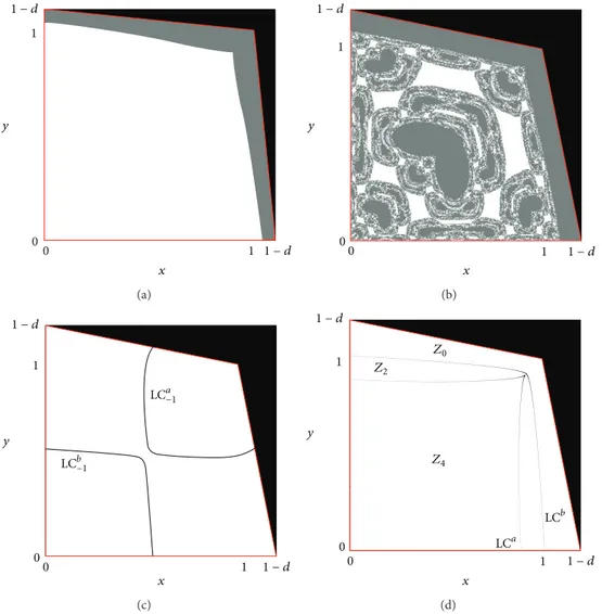
The feasible set of system𝑇 is depicted in white in Figures

1(a)and1(b)for two different parameter constellations, while

the unfeasible points belonging to𝑄 are depicted in grey. The

following evidence can be immediately observed: similarly

to the substitutability case, (i) set𝐷 is nonempty such that

𝐷 ⊂ 𝑄 and (ii) set 𝐷 may have a simple structure (as in

Figure 1(a)) or a complex structure (as inFigure 1(b)). The

first evidence can be easily demonstrated by considering that

the origin is a feasible point and that there exists a𝜂 > 0 small

enough such that(1 − 𝜂, 1 − 𝜂) is not a feasible point.

With regard to the study of the structure of the feasible set, a numerical procedure based on the study of the properties of the critical curves can be used (see, e.g., [15–17]). By taking into account the results proved in Fanti et al. [13], it is easy to

verify that𝑇 is of 𝑍₄−𝑍₂−𝑍₀type since𝑄 can be subdivided

into regions whose points have4, 2, or 0 preimages, and the

boundaries of such regions are characterised by the existence of at least two coincident preimages.

We denote the critical curve of rank-1 by LC (it represents the locus of points that have two or more coincident

preim-ages) and the curve of merging preimages by LC₋₁; that is, the

(3)

0 0 1 1 − d 1 1 − d y x (a) 1 − d 1 − d 1 1 y 0₀ x (b) 0 0 1 1 1 − d 1 − d y x LCb −1 LCa −1 (c) 0 1 − d 1 − d 0 1 1 Z2 Z4 Z0 y x LCb LCa (d)

Figure 1: (a), (b). The feasible set𝐷 ⊂ 𝑄 is depicted in white; the gray points are initial conditions producing unfeasible trajectories. (a) 𝛼 = 1.5, 𝑑 = −0.1, 𝑤 = 0.5, and 𝑏₁= 𝑏₂= 0.2. (b) 𝛼 = 1.5, 𝑑 = −0.2, 𝑤 = 0.5, and 𝑏₁= 𝑏₂= 0.2. (c) Critical curves of rank-0, LC₋₁, for system 𝑇 and the parameter values as in (b). (d) Critical curves of rank-1, LC = 𝑇(LC−1), for the same parameter values as in panel (c). These curves

separate the plane into the regions𝑍₄,𝑍₂, and𝑍₀, whose points have a different number of preimages.

𝐽 (𝑥, 𝑦) = ( 1 + 𝛼 (1 − 4𝑥 − 𝑑 (1 − 𝑦) + 𝑤 1 − 𝑑2 −𝑏1(1 + 𝑑) (1 − 𝑦) (2 + 𝑥 − 𝑦)_{(1 − 𝑑) (2 − 𝑥 − 𝑦)}3 ) 𝛼𝑥 (_{1 − 𝑑}𝑑 2 − 𝑏1 (1 + 𝑑) (𝑥 − 𝑦) (1 − 𝑑) (2 − 𝑥 − 𝑦)3) 𝛼𝑦 ( 𝑑 1 − 𝑑2 − 𝑏2 (1 + 𝑑) (𝑦 − 𝑥) (1 − 𝑑) (2 − 𝑥 − 𝑦)3) 1 + 𝛼 ( 1 − 4𝑦 − 𝑑 (1 − 𝑥) + 𝑤 1 − 𝑑2 − 𝑏2(1 + 𝑑) (1 − 𝑥) (2 − 𝑥 + 𝑦) (1 − 𝑑) (2 − 𝑥 − 𝑦)3 ) ), (7)

is the Jacobian matrix of system𝑇 (see Figures1(c)and1(d)).

The study of the structure of set 𝐷 is of interest from

both economic and mathematical perspectives, since the long-term evolution of the economic system becomes

path-dependent, and a thorough knowledge of the properties of𝐷

becomes crucial in order to predict the system’s feasibility.

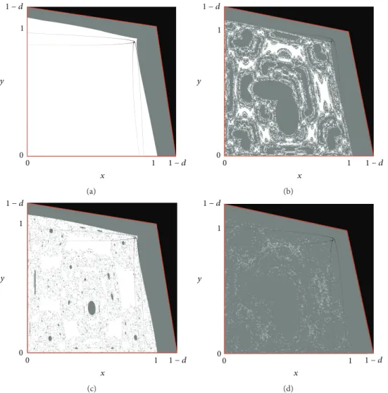
We now fix all parameter values but𝑑. Then, as is shown

in Figures2(a)and 2(b), if𝑑 = −0.15, set 𝐷 has a simple

structure (connected set), while when𝑑 = −0.2, set 𝐷 consists

of infinitely many nonconnected sets. This is due to the fact

that the LC𝑏curve moves upwards as parameter𝑑 decreases

and consequently a threshold value𝑑 ≃ −0.1551 does exist

such that a contact between a critical curve and the boundary of the feasible set occurs. This contact bifurcation causes

the change of 𝐷 from a connected set to a nonconnected

set. In fact, a portion of the unfeasible set enters in a region characterised by a high number of preimages so that new components of the unfeasible set suddenly appear

after the contact (inFigure 2(c), the feasible set is depicted

immediately after the contact bifurcation creating grey holes inside the white region). The complexity of the structure of

(4)

1 − d 1 − d 1 1 y 0 0 x (a) 1 − d 1 − d 1 1 y 0 0 x (b) 1 − d 1 1 − d 1 y 0 0 x (c) 1 − d 1 y 0 x 1 − d 1 0 (d)

Figure 2: Parameter values:𝛼 = 1.5, 𝑤 = 0.5, 𝑏₁ = 0.4, and 𝑏₂ = 0.2. (a) 𝐷 has a simple structure (𝑑 = −0.15). (b) 𝐷 has a complex structure (𝑑 = −0.2). (c) Set 𝐷 after the contact bifurcation (𝑑 = −0.16): gray holes are depicted. (d) Immediately before the final bifurcation (𝑑 = −0.216) almost all trajectories are unfeasible.

increases too (i.e., the set of initial conditions generating unfeasible trajectories); however, it can be also observed that

if𝑑 decreases further, a final bifurcation occurs. In fact, as

𝑑 crosses a value 𝑑 ≃ −0.218, almost all trajectories become

unfeasible (seeFigure 2(d)).

Notice that in the simulations presented inFigure 2we

have assumed𝑏₁ ̸= 𝑏₂. However, a similar behaviour holds

also when 𝑏₁ = 𝑏₂: in this case, the contact bifurcation

between the critical set and the boundary of the feasible set occurs at two points that are symmetric with respect to the main diagonal, so that the resulting feasible set is symmetric

too (see Figures1(a)and1(b)). The previous arguments show

that the bifurcations concerning the structure of the feasible set is strictly related to the value of the two key parameters

𝑑 and 𝑏_𝑖, which represent the degree of horizontal product

differentiation and the level of market share bonuses. The following results can be proved.

Proposition 1. Let 𝑇 be the dynamic system given by(6).

(i) If𝑑 → −1+, then𝐷 = {(0, 0)}.

(ii) If𝑏_𝑖 → +∞, 𝑖 = 1, 2, then 𝐷 = {(0, 0)}.

Proof. (i) If𝑑 → −1+, then𝑄 → 𝐼 = {(𝑥, 𝑦) ∈ R2₊: 𝑥 + 𝑦 ≤ 2, 𝑥 ≥ 0, 𝑦 ≥ 0}. Observe first that it must be 𝑥 + 𝑦 < 2

for𝑇 being well defined and that (0, 0) ∈ 𝐷, and hence we

consider initial conditions such that𝑥(0) + 𝑦(0) < 2 and at

least one component of(𝑥(0), 𝑦(0)) is strictly positive. Taking

into account system(6), it can be observed that

𝑥 (1) + 𝑦 (1) = 𝑥 (0) + 𝑦 (0) + 𝜔 (𝑑, 𝑥 (0) , 𝑦 (0)) (8)

and that∀(𝑥(0), 𝑦(0)) ∈ 𝑄 : 𝑥(0) + 𝑦(0) < 2 and 𝑥(0) +

𝑦(0) ̸= 0; if 𝑑 → −1+_{, then}_{𝜔(𝑑, 𝑥(0), 𝑦(0)) diverges; that is,}

(𝑥(0), 𝑦(0)) produces an unfeasible trajectory.

(ii) This statement can be proved simply considering the

limits lim_𝑏₁_{→ +∞}𝑥(1) and lim_𝑏₂_{→ +∞}𝑦(1) for any given initial

point(𝑥(0), 𝑦(0)) ∈ 𝑄, 𝑥(0) + 𝑦(0) ̸= 0.

According to Proposition 1, if 𝑏_𝑖 is high enough or

products tend to be complements (𝑑 is low enough), the feasible set is consists of only the origin. This result confirms the one obtained in Fanti et al. [13] for the substitutability case; that is, economic meaningful dynamics are produced only when the degree of complementarity or substitutability

(5)

between products is not too high. More precisely, in the case under investigation, economically meaningful

long-term dynamics can be produced only for𝑑 ∈ 𝐼₋(0) and 𝑏_𝑖 ∈

𝐼₊(0) (𝑖 = 1, 2), thus confirming the numerical experiments

previously presented.

By taking into account the above-mentioned arguments, in what follows we will focus on the study of the dynamics

produced by𝑇 by assuming that 𝑏_𝑖is sufficiently small and𝑑

is sufficiently high.

4. Fixed Points, Invariant Sets, and

Local Stability

Let 𝑇 be the dynamic system given by(6) and consider a

feasible initial condition. We now recall the results proved in Fanti et al. [13] concerning fixed points and other invariant

sets of𝑇 for 𝑑 ∈ (0, 1). It can be verified that they still hold

also when𝑑 ∈ (−1, 0]. We here present a sketch of the proof

and we refer to Fanti et al. [13] for a further discussion.

Remark 2. Let𝑇 be given by(6). Then, one has the following.

(i)𝐼_𝑥= {(𝑥, 𝑦) : 0 ≤ 𝑥 ≤ 1 − 𝑑, 𝑦 = 0} and 𝐼_𝑦= {(𝑥, 𝑦) :

0 ≤ 𝑦 ≤ 1 − 𝑑, 𝑥 = 0} are invariant sets. The dynamics

of𝑇 on such sets are governed by 𝜙_𝑥 = 𝑥𝐹(𝑥, 0) and

𝜙𝑦 = 𝑦𝐺(0, 𝑦) and they can be complex; in any case,

𝐼_𝑥and𝐼_𝑦are repellor.

(ii) If𝑏₁ = 𝑏₂ = 𝑏, then also Δ = {(𝑥, 𝑦) ∈ R2₊ : 𝑥 =

𝑦, 𝑥 ∈ [0, 1)} is an invariant set. The dynamics of 𝑇 on

such a set are governed by𝜙(𝑥) = 𝑥[1 + (𝛼/(1 − 𝑑))

(((1 − 𝑑)(1 − 𝑥) − 𝑥 + 𝑤)/(1 + 𝑑) − 𝑏((1 + 𝑑)/4(1 − 𝑥)))]

and they can be complex; furthermore,Δ can be an

attracting set.

(iii) The origin𝐸₀= (0, 0) is a fixed point for all parameter

values; it can be a stable node, an unstable node, or

a saddle point. Up to two more fixed points on 𝐼_𝑦

and𝐼_𝑥may be owned. They are given by𝐸₁ = (0, 𝑦₀)

and𝐸₂= (𝑥₀, 0) and can be unstable nodes or saddle

points.

(iv) If𝑏₁ = 𝑏₂ = 𝑏, then 𝑇 admits a unique interior fixed

point 𝐸∗_𝑏 = (𝑥_𝑏∗, 𝑥∗_𝑏) for all 𝑏 < 4(1 − 𝑑 + 𝑤)/

(1 + 𝑑)2 _{= 𝑏, where 𝑥}∗

𝑏 = 1 − ((1 − 𝑤) +

√(1 − 𝑤)2_{+ 𝑏(2 − 𝑑)(1 + 𝑑)}2_{)/2(2 − 𝑑). 𝐸}∗

𝑏 can be a

stable node, an unstable node, or a saddle point.

Proof. Consider the system𝑇 given by(6).

(i)𝑇(𝑥, 0) = (𝑥󸀠, 0) and 𝑇(0, 𝑦) = (0, 𝑦󸀠); that is, 𝐼_𝑥and𝐼_𝑦

are invariant, and consequently the dynamics of𝑇 on

such lines are governed by the two one-dimensional

maps𝜙_𝑥 = 𝑥𝐹(𝑥, 0) and 𝜙_𝑦 = 𝑦𝐺(0, 𝑦). As both 𝜙_𝑥

and𝜙_𝑦are unimodal for suitable parameter values (as

proved in [13]), complex dynamics can be produced.

𝐼_𝑥and𝐼_𝑦are repellor as the eigenvalue of𝐽(𝑥, 0) and

𝐽(0, 𝑦) associated with the direction orthogonal to each semiaxis is greater than one for all parameter values.

(ii) Assume𝑏₁ = 𝑏₂ = 𝑏; then, 𝑇(𝑥, 𝑥) = (𝑥󸀠, 𝑥󸀠), and

henceΔ is invariant and the dynamics of system 𝑇 on

Δ are governed by 𝜙(𝑥) = 𝑥𝐹(𝑥, 𝑥). Given the

proper-ties of𝜙(𝑥) studied in Fanti et al. [13],

nonmonoton-icity can occur for suitable parameter values and

complex dynamics may emerge. Finally,Δ can be an

attracting set as the eigenvalue of𝐽(𝑥, 𝑥) associated

with the eigenvector orthogonal to the diagonal may be less than one in modulus (see again Fanti et al. [13]).

(iii) Since𝑇(0, 0) = (0, 0), 𝐸₀is a fixed point; furthermore,

while considering𝐽(0, 0), it can be observed that 𝐸₀

can be a stable node, an unstable node, or a saddle

point. By solving𝜙_𝑥 = 𝑥 and 𝜙_𝑦 = 𝑦 and following

Fanti et al. [13], it can be easily verified that up to two

positive solutions exist, namely,𝐸₁and𝐸₂; such fixed

points cannot be stable nodes as𝐼_𝑥and𝐼_𝑦are repellor.

(iv) Assume𝑏₁= 𝑏₂= 𝑏; then, by solving equation 𝜙(𝑥) =

𝑥 it can be verified that it admits a unique positive

feasible solution𝑥∗_𝑏 iff𝑏 < 𝑏 (see Fanti et al. [13] for

more details); as each eigenvalue of𝐽(𝑥∗_𝑏, 𝑥∗_𝑏) can be

greater or less than one in modulus, then𝐸∗_𝑏 can be a

stable node, an unstable node, or a saddle point.

The question of the existence of an interior fixed point

in the general case𝑏₁ ̸= 𝑏₂(i.e., with different market share

bonuses) cannot be addressed analytically. However, it will be discussed later in the paper by using numerical techniques.

By taking into account parts (i) and (iii) inRemark 2, in what

follows we will focus on the study of the dynamics produced

by𝑇 for a feasible initial condition belonging to the interior

of𝑄, thus focusing on economically meaningful initial states.

5. Synchronisation and Multistability

In order to study the evolution of system𝑇 when products are

independent or complementary and compare this case with that of substitutable goods, we concentrate on the particular

case of identical market share bonuses; that is,𝑏₁= 𝑏₂= 𝑏. As

a consequence, system𝑇 in(6)takes the symmetric form𝑇_𝑏

given by 𝑇_𝑏: { { { { { { { { { { { { { { { { { { { { { { { { { { { { { { { { { { { { { { { { { { { { { { { { { 𝑥󸀠_{= 𝑥𝑓 (𝑥, 𝑦)} = 𝑥 [ 1 + 𝛼 (1 − 2𝑥 − 𝑑 (1 − 𝑦) + 𝑤 1 − 𝑑2 − 𝑏 (1 + 𝑑) (1 − 𝑦) (1 − 𝑑) (2 − 𝑥 − 𝑦)2)] 𝑦󸀠= 𝑦𝑔 (𝑥, 𝑦) = 𝑦 [ 1 + 𝛼 (1 − 2𝑦 − 𝑑 (1 − 𝑥) + 𝑤 1 − 𝑑2 − 𝑏 (1 + 𝑑) (1 − 𝑥) (1 − 𝑑) (2 − 𝑥 − 𝑦)2)] . (9)

(6)

Since map𝑇_𝑏is symmetric, that is, it remains the same when the players are exchanged, then either an invariant set

of the map is symmetric with respect toΔ or its symmetric set

is invariant. By considering part (iv) inRemark 2, the local

stability analysis of the unique interior fixed point𝐸∗_𝑏 can

be carried out by considering the Jacobian matrix associated

with system𝑇_𝑏given by

𝐽_𝑏(𝑥, 𝑦) = (1 + 𝛼 ( 1 − 4𝑥 − 𝑑 (1 − 𝑦) + 𝑤 1 − 𝑑2 −𝑏 (1 + 𝑑) (1 − 𝑦) (2 + 𝑥 − 𝑦)_{(1 − 𝑑) (2 − 𝑥 − 𝑦)}3 ) 𝛼𝑥 (_{1 − 𝑑}𝑑 2 − 𝑏_{(1 − 𝑑) (2 − 𝑥 − 𝑦)}(1 + 𝑑) (𝑥 − 𝑦) 3) 𝛼𝑦 ( 𝑑 1 − 𝑑2 − 𝑏 (1 + 𝑑) (𝑦 − 𝑥) (1 − 𝑑) (2 − 𝑥 − 𝑦)3) 1 + 𝛼 ( 1 − 4𝑦 − 𝑑 (1 − 𝑥) + 𝑤 1 − 𝑑2 − 𝑏 (1 + 𝑑) (1 − 𝑥) (2 − 𝑥 + 𝑦) (1 − 𝑑) (2 − 𝑥 − 𝑦)3 ) ) . (10) Let 𝐽₁(𝑥) = 1 +_{1 − 𝑑}𝛼 ₂ ⋅4 (4 − 𝑑) (1 − 𝑥)3+ 4 (𝑤 − 3) (1 − 𝑥)2− 𝑏 (1 + 𝑑)2 4 (1 − 𝑥)2 , 𝐽2(𝑥) =_{1 − 𝑑}𝛼𝑑₂𝑥. (11) Then, the Jacobian matrix evaluated at a point on the diagonal Δ is of the kind

𝐽_𝑏(𝑥, 𝑥) = (𝐽1(𝑥) 𝐽2(𝑥)

𝐽2(𝑥) 𝐽1(𝑥)) ,

(12)

so that the eigenvalues of𝐽_𝑏(𝑥, 𝑥) are both real and given by

𝜆_𝑏‖(𝑥) = 𝐽₁(𝑥) + 𝐽₂(𝑥) ,

𝜆_𝑏⊥(𝑥) = 𝐽₁(𝑥) − 𝐽₂(𝑥) , (13)

while the corresponding eigenvectors are, respectively, given

byV_𝑏‖ = (1, 1) and V_𝑏⊥= (1, −1).

The eigenvalues evaluated at the fixed point 𝐸∗_𝑏 are,

respectively,

𝜆_𝑏‖(𝐸∗_𝑏) = 𝐽₁(𝐸∗_𝑏) + 𝐽₂(𝐸∗_𝑏) ,

𝜆_𝑏⊥(𝐸∗_𝑏) = 𝐽₁(𝐸∗_𝑏) − 𝐽₂(𝐸∗_𝑏) . (14)

Thus,𝐸∗_𝑏 can be attracting for suitable values of parameters

such that both𝜆_‖(𝐸∗_𝑏) and 𝜆_⊥(𝐸∗_𝑏) belong to the set (−1, 1).

Different from the case in which products are substitutes, the following Proposition can easily be verified.

Proposition 3. If 𝑑 = 0, then 𝜆_𝑏‖(𝐸∗_𝑏) = 𝜆_𝑏⊥(𝐸∗_𝑏); if 𝑑 ∈

(−1, 0), then 𝜆_𝑏‖(𝐸∗_𝑏) < 𝜆_𝑏⊥(𝐸∗_𝑏).

Proof. If 𝑑 = 0, then 𝐽₂(𝑥) = 0 ∀𝑥, and consequently

𝜆_𝑏‖(𝐸∗

𝑏) = 𝜆𝑏⊥(𝐸∗𝑏); if 𝑑 ∈ (−1, 0), then 𝐽2(𝑥) < 0 ∀𝑥 > 0,

and hence𝜆_𝑏‖(𝐸∗_𝑏) < 𝜆_𝑏⊥(𝐸∗_𝑏).

From Proposition 3 it follows that if 𝑑 = 0, then

the interior fixed point is a stable or an unstable node.

Furthermore, conditions𝜆_𝑏‖(𝐸∗_𝑏) > 1 or 𝜆_𝑏⊥(𝐸∗_𝑏) < −1 are

sufficient for𝐸_𝑏∗to be an unstable node.

The following condition for the local stability of 𝐸∗_𝑏

(which holds if products are substitutes) applies also to the

case𝑑 ∈ (−1, 0] and it can be recalled below (see Fanti et al.

[13] for the proof).

Proposition 4. Let system 𝑇_𝑏be given by(9). Then a𝜖 > 0 does

exist such that𝐸∗_𝑏is locally asymptotically stable∀𝑏 ∈ (𝑏−𝜖, 𝑏), given the other parameter values.

By taking into account Propositions 3 and 4, a

suffi-cient condition for 𝐸∗_𝑏 to be locally stable for 𝑑 = 0 is

𝑏 → 4(1 + 𝑤)−. In this case, given the geometric properties

of map𝜙(𝑥) described in Fanti et al. [13], the initial conditions

belonging toΔ converge to 𝑥∗_𝑏 with independent products.

In addition, the trajectories starting from initial conditions

close to it, that is, (𝑥(0), 𝑦(0)) ∈ 𝐼(𝐸∗_𝑏, 𝑟), with 𝑥(0) ̸=

𝑦(0), also converge to 𝐸∗

𝑏. This behaviour occurs as long

as 𝑑 ∈ 𝐼₋(0), while, as 𝑑 decreases, the fixed point loses

its stability firstly along the diagonal, thus giving rise to a different scenario compared to that presented in Fanti et al. [13] for the substitutability case.

Definition 5. A feasible trajectory 𝜓_𝑡 = {𝑥(𝑡), 𝑥(𝑡)}∞_𝑡=0, (𝑥(0), 𝑥(0)) ∈ Δ, is called synchronised trajectory. A feasible

trajectory starting from(𝑥(0), 𝑦(0)) ∈ 𝐷 − Δ, that is, with

𝑥(0) ̸= 𝑦(0), is synchronised if |𝑥(𝑡)−𝑦(𝑡)| → 0 as 𝑡 → +∞. With regards to the dynamics of synchronised

trajecto-ries, we first recall the result proved inProposition 1.

An attractor𝐴 located on the invariant set Δ exists for

𝑇_𝑏 if products are not too complementary (𝑑 is not too

low) and the market share bonus 𝑏 is not too large (see

Figures 3(a)and 3(c)). This fact can also be confirmed by

considering the following properties of map𝜙(𝑥): 𝜙(0) = 0,

lim_{𝑥 → 1}−𝜙(𝑥) = −∞, 𝜙󸀠(0) > 1 ∀𝑏 ∈ (0, 𝑏), 𝜙󸀠󸀠(𝑥) < 0 ∀𝑥 ∈

[0, 1). As a consequence, there exists a unique 𝑥₋∈ (0, 1) such

that𝜙(𝑥₋) = 0 and a unique maximum point 𝑥_𝑀 ∈ (0, 𝑥₋)

such that𝜙(𝑥_𝑀) is the maximum value of 𝜙 in [0, 1). This

implies that 𝜙 is unimodal in [0, 𝑥₋]. By considering that

𝜙(𝑥_𝑀) increases when 𝑑 decreases and 𝜙(𝑥_𝑀) → +∞ if 𝑑 →

−1, then a 𝑑 does exist such that 𝜙(𝑥_𝑀) > 𝑥₋if−1 < 𝑑 < 𝑑

(seeFigure 3(b)). On the other hand, by considering the role

of parameter𝑏, a cascade of period doubling bifurcations is

(7)

d x b = 0.8 b = 2.5 0.8 0 0 −0.35 d x 1 0 0 −0.25 (a) 0 1 1 0 x 𝜙 (x) d = −0.2 Δ d = −0.4 (b) x x d = −0.05 d = −0.2 10.625 6.8698 0 0 0 0 1 1 b b (c)

Figure 3: Parameter values:𝑤 = 0.5, 𝛼 = 1.5. (a) One-dimensional bifurcation diagrams with respect to 𝑑 for two fixed 𝑏 values. (b) Map 𝜙 is plotted for different𝑑 values and 𝑏 = 1. (c) One-dimensional bifurcation diagrams with respect to 𝑏 (0 < 𝑏 < 𝑏) for two fixed 𝑑 values.

By taking into account the previous results and looking

at the one-dimensional bifurcation diagrams in Figures3(a)

and 3(c), it can be observed that synchronised trajectories

converge to the unique interior fixed point if𝑏 is close to 𝑏 (the

manager bonus is close to its upper limit). In addition, similar to what occurs with the logistic map, cycles can emerge due

to period doubling bifurcation of𝜙 when 𝑑 decreases (i.e., the

degree of complementarity between products increases). This evidence is also confirmed when products are substitutes, thus proving that complexity in synchronised trajectories arises when moving away from the hypothesis of independent products.

Let us consider now a duopoly with identical players that

start from different feasible initial conditions and let𝐴 ⊆ Δ be

an attracting set of𝜙. If 𝐴 = 𝐸_𝑏∗for𝑑 = 0, then by considering

(13)andProposition 3the following proposition holds.

Proposition 6. Let 𝑥∗

𝑏be an attracting fixed point of𝜙 for 𝑑 =

0. Then, 𝐸∗

𝑏is an attracting fixed point of𝑇𝑏and∃𝑑−< 0 such

that𝐸∗_𝑏is an attracting fixed point of 𝑇_𝑏 ∀𝑑 ∈ (𝑑₋, 0)∩(−1, 0).

At𝑑 = 𝑑₋, the fixed point𝐸∗_𝑏 loses stability along the diagonal.

Proof. Let𝑑 = 0 and assume that 𝑥∗_𝑏 is an attracting fixed

point of𝜙; that is, 𝜙󸀠(𝑥_𝑏∗) = 𝜆_𝑏‖(𝐸∗_𝑏) ∈ (−1, 1). Since 𝜆_𝑏‖(𝐸∗_𝑏) =

𝜆_𝑏⊥(𝐸∗

𝑏), then 𝐸∗𝑏 is an attracting fixed point of𝑇𝑏. As both

𝜆_𝑏‖(𝐸∗

𝑏) and 𝜆𝑏⊥(𝐸∗𝑏) are continuous with respect to 𝑥∗𝑏 and

𝑑, then ∃𝐼₋(0) such that |𝜆_𝑏‖(𝐸∗

𝑏)| < 1 and |𝜆𝑏⊥(𝐸∗𝑏)| < 1

∀𝑑 ∈ (𝑑₋, 0)∩(−1, 0), and 𝐸∗_𝑏is an attracting fixed point of𝑇_𝑏.

Finally, since𝜆_𝑏‖(𝐸∗_𝑏) < 𝜆_𝑏⊥(𝐸∗_𝑏) ∀𝑑 ∈ (−1, 0) and they are

both increasing with respect to𝑑, then as 𝑑 crosses 𝑑₋ the

eigenvalue𝜆_𝑏‖(𝐸∗_𝑏) must cross −1; that is, 𝐸∗_𝑏loses its stability

along the diagonal.

According toProposition 6, if synchronised trajectories

converge to 𝑥∗_𝑏 for 𝑑 = 0, then trajectories starting from

feasible initial conditions close to it, with 𝑥(0) ̸= 𝑦(0),

are synchronised in the long term as long as 𝑑 ∈ 𝐼₋(0).

(8)

along the diagonal. This contrasts with the result obtained in Fanti et al. [13] where products are substitutes. In fact, if 𝑑 passes from zero to positive values, the fixed point first loses transverse stability and consequently the trajectories are not synchronised. Therefore, synchronisation in this model is strictly related to the assumption of complementarity between products.

If𝐴 consists of a 𝑚-cycle, then, similarly to what happens

for the fixed point, several numerical computations show

that if 𝐴 is a 𝑚-cycle for 𝑑 = 0, then the 𝑚-cycle loses

stability firstly along the diagonal when 𝑑 decreases, so

that synchronisation may occur. Different from the case of substitutability, this evidence confirms that when products are complements, players may coordinate their behaviour towards a situation in which prices are equal (and the market is equally shared). In our analysis it is also stressed that the

emergence of synchronisation with negative values of𝑑 also

confirms the result obtained in Fanti et al. [18] with profit-maximising firms.

Consider now a more complex situation; that is,𝐴 is a

chaotic attractor onΔ. In order to study its transverse stability,

it is possible to use the procedure proposed in Bischi et al. [14], Bischi and Gardini [19], and Bignami and Agliari [20]. Recall that the transverse Lyapunov exponent is defined as follows:

Λ_𝑏⊥ = lim 𝑁 → ∞ 1 𝑁 𝑁 ∑ 𝑛=0 ln 󵄨󵄨_󵄨󵄨𝜆_𝑏⊥(𝑥_𝑛)󵄨󵄨󵄨󵄨 , (15)

where𝑥₀∈ 𝐴 and 𝑥_𝑛is a generic trajectory generated by𝜙.

If𝑥₀belongs to a generic aperiodic trajectory embedded

within the chaotic set𝐴, then Λ_𝑏⊥ is the natural transverse

Lyapunov exponent Λ𝑛_𝑏⊥, where natural indicates that the exponent is computed for a typical trajectory taken in

the chaotic attractor 𝐴. Since infinitely many cycles (all

unstable along the diagonal) are embedded inside the chaotic

attractor 𝐴, a spectrum of transverse Lyapunov exponents

can be defined and the natural transverse Lyapunov exponent represents a sort of weighted balance between the transversely repelling and transversely attracting cycles. If all cycles

embedded in𝐴 are transversely stable, that is Λmax_𝑏⊥ < 0, then

𝐴 is asymptotically stable in the Lyapunov sense for the

two-dimensional map𝑇_𝑏. Nevertheless, it may occur that some

cycles embedded in the chaotic set𝐴 become transversely

unstable; that is, Λmax_𝑏⊥ > 0, while Λ𝑛_𝑏⊥ < 0. In such a

case,𝐴 is not stable in the Lyapunov sense but it is a stable

attractor in the Milnor sense. If a Milnor attractor of 𝑇_𝑏

exists, then some transversely repelling trajectories can be embedded in a chaotic set which is attracting only on average. In addition, such transversely repelling trajectories can be

reinjected towardΔ so that their behaviour is characterised

by some bursts far from the diagonal, before synchronization or convergence towards a different attractor. This situation is called on-off intermittency.

In order to investigate the existence of a Milnor attractor 𝐴, we numerically estimate the natural transverse Lyapunov

exponentΛ𝑛_𝑏⊥, represented with respect to𝑏 inFigure 4(a)

for a fixed negative value of𝑑. It is possible to observe that it

can take negative values. As an example, we consider𝑏 = 2.07

at whichΛ𝑛_𝑏⊥ < 0 while Λmax_𝑏⊥ > 0 and the one-dimensional

map𝜙 exhibits a 4-piece chaotic attractor. 𝐴 is an attractor

of system𝑇_𝑏belonging to the diagonal (seeFigure 4(b)), but

a trajectory starting from an initial condition that does not belong to the diagonal has a long transient before converging

to𝐴 (seeFigure 4(c)). In fact, by considering the difference

𝑥(𝑡) − 𝑦(𝑡) for any 𝑡 we can observe that the transient part of the trajectory is characterised by several bursts away from Δ. The typical on-off intermittency phenomenon occurs. The

whole trajectory starting from𝑥(0) = 0.1 and 𝑦(0) = 0.2 is

shown inFigure 4(d).

The study of the geometrical properties of the critical lines may be used to estimate the maximum amplitude of the bursts by obtaining the boundary of a compact trapping region of the phase plane in which the on-off intermittency phenomena are confined. Following Mira et al. [21], we obtain

the boundary of the absorbing area inFigure 4(e)for the case

presented inFigure 4(d). Observe that such a region contains

the whole trajectory presented inFigure 4(d). However, not

all trajectories are synchronised as𝑇_𝑏also admits a coexisting

attractor, that is, a2-period cycle whose basin is depicted in

orange inFigure 4(f).

If 𝑇_𝑏 admits an attractor 𝐴 ⊂ Δ and there exist

feasible trajectories starting from interior points that are not synchronised, then the question of multistability has to be considered. In fact, several attractors may coexist (each of which with its own basin of attraction) so that the selected long-term state becomes path dependent, as in the situation

shown inFigure 4(f). In this case, the structure of the basins

of different attractors becomes crucial to predict the

long-term outcome of the economic system. InFigure 5(a), the

unique Nash equilibrium is locally stable, as the market share bonus is close to its upper limit. It is also globally stable, in the sense that it attracts all feasible trajectories taken into

the interior of the feasible set𝐷 (that represents economic

meaningful initial conditions).

If we compute𝜕𝑏/𝜕𝑑, then it is possible to observe that

𝑏 increases as 𝑑 decreases, and 𝑏 → +∞ as 𝑑 → −1+_.

As a consequence, in order to obtain the convergence to the

unique Nash equilibrium,𝑏 must be set at higher levels as the

degree of horizontal product differentiation𝑑 decreases (i.e.,

products tend to be more complementary). Furthermore, if

products are complements, then𝜆_𝑏‖crosses−1 as 𝑏 decreases

and a flip bifurcation occurs along the invariant setΔ; that is,

a 2-period cycle appears close to the fixed point and it is stable along the diagonal. By taking into account the result proved

in Proposition 3, when this bifurcation occurs, 𝜆_𝑏⊥ is still

smaller than1 in modulus and consequently (immediately

after the first flip bifurcation) the2-period cycle attracts all

interior feasible trajectories. However, if𝑏 is still decreased,

a period doubling bifurcation cascade occurs along the diagonal, so that more complex bounded attractors (such as

periodic cycles) may exist on Δ around the unstable Nash

equilibrium. As a consequence, the long-term synchronised dynamics may be characterised by bounded periodic (or even aperiodic) oscillations around the Nash equilibrium.

If the attractor𝐴 is transversely unstable, the situation may

become very complicated, as it is shown inFigure 5(b)where

a2-period cycle attracts all synchronised trajectories, while

(9)

2 2.01 2.02 2.03 2.04 2.05 2.06 2.07 2.08 2.09 2.1 0.4 0.3 0.2 0.1 0 −0.1 −0.2 b (a) 0 1.2 1.2 0 y x (b) 0 8000 −0.5 0 0.5 t x (t ) − y (t ) (c) 1.2 0 y 0 1.2 x (d) y x 0 1.2 0 1.2 (e) y x 0 1 0 1 (f)

Figure 4: Parameter values:𝛼 = 1.5, 𝑑 = −0.2, and 𝑤 = 0.5. (a) The natural transverse Lyapunov exponent with respect to parameter 𝑏. (b) Four-piece chaotic attractor𝐴 of system 𝑇_𝑏belonging to the diagonal for𝑏 = 2.07. (c) Bursts away from the diagonal before synchronization for𝑏 = 2.07, 𝑥(0) = 0.1, and 𝑦(0) = 0.2. (d) The whole trajectory starting from initial condition as in (c) and converging to the attractor in (b). (e) The minimal absorbing area in which on-off intermittency phenomenon occurs for the same parameters as in (c). (f) The attractor𝐴 coexists with an attracting 2-period cycle for𝑏 = 2.07.

(10)

0 1.2 0 1.2 E∗b y x (a) 0 1.2 0 1.2 y x (b) 0 0.8 0 0.8 y x (c) 0 1 0 1 x y (d)

Figure 5: Parameter values:𝛼 = 1.5 and 𝑤 = 0.5. (a) The white region represents the basin of 𝐸∗_𝑏for𝑏 = 5.1 and 𝑑 = −0.2. (b) A 4-period cycle together with a2-period cycle coexists with the attractor 𝐴 belonging to the diagonal (a two-period cycle) for 𝑏 = 2.4 and 𝑑 = −0.2. (c) For𝑏 = 2.3, a 4-piece quasi-periodic attractor has been created, 𝑑 = −0.2. (d) A particular scenario is presented for 𝑏 = 0.2 in the case of independent products𝑑 = 0.

whose basin is depicted in orange and a4-period cycle whose

basin is depicted in yellow; note that the periodic points are in symmetric position with respect to the diagonal. As the

parameter𝑏 decreases, a further flip bifurcation occurs and

a4-period cycle is created on the diagonal (seeFigure 5(c));

furthermore, the4-period cycle existing out of the diagonal

becomes a stable focus and then undergoes a Neimark-Sacker

bifurcation at which it becomes a4-cyclic attractor formed

by a4-piece quasi-periodic attractor (green basin) coexisting

with a2-period cycle (orange basin), while synchronisation

is avoided. This is how the situation presented inFigure 4(f)

is approached: a final bifurcation that causes the transition to more complex basin boundaries occurs. Consequently to the

final state sensitivity it is impossible to predict the long-term

outcomes of the economy.

Finally, we consider the case in which products are independent from each other and each manager behaves as a monopolist (𝑑 = 0). When a flip bifurcation along the

diagonal creates a 𝑘-period cycle, it can be observed that

a𝑘-period cycle is simultaneously created out of the diagonal

as the eigenvalues of cycles embedded into the diagonal are identical. As a consequence, any period doubling bifurcation

along Δ is associated with a period doubling bifurcation

orthogonal to Δ. A similar phenomenon of multistability

is presented in Bischi and Kopel [22]. This case is shown

inFigure 5(d): the green points represent initial conditions

converging to a 4-period cycle on the diagonal while the

yellow points represent initial conditions converging to a 4-period cycle out of the diagonal. This scenario occurs

when the2-period cycle along the diagonal undergoes the

second period doubling bifurcation: two stable 4-period

cycles are created, one along the diagonal (red points) and one with periodic points symmetric to it (black points); these

two stable cycles coexist with the2-period cycle previously

created out of the diagonal (white points). Observe that an economy starting far away from the diagonal may become

synchronised, as the basin of attraction 𝐴 on the diagonal

(11)

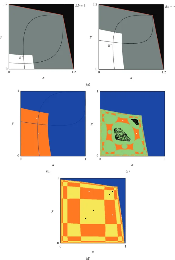
1.2 0 1.2 0 y x 1.2 0 1.2 0 y x E∗ E∗ Δb = −3 Δb = 3 (a) 1 0 0 y x 1 (b) 1 0 1 0 y x (c) 1 0 1 0 y x (d)

Figure 6: (a) Parameter values:𝛼 = 1.5, 𝑤 = 0.5, 𝑏 = 5.1, and 𝑑 = −0.2. The Nash equilibrium for positive and negative values of Δ𝑏. (b) If Δ𝑏 = −0.3, the Nash equilibrium is unstable and a 2-period cycle is globally stable. (c) A complex attractor 𝐴 (black points) coexists with a 2-period cycle (white points) if 𝛼 = 1.5, 𝑤 = 0.5, 𝑏 = 2.07, 𝑑 = −0.2, and Δ𝑏 = 0.15. (d) Coexisting attractors if 𝑏 = 0.2, 𝑑 = 0 while Δ𝑏 = 0.01.

(12)

relevant from an economic point of view. In fact, it implies coordination even though the manager hired in each firm behaves as a monopolist in his own market.

5.1. The Asymmetric Case. We now consider the case in which

managers’ bonuses are evaluated differently; that is,𝑏₁ ̸= 𝑏₂.

Obviously, in this caseΔ is no longer invariant (i.e., if the firms

start from the same initial feasible condition(𝑥(0), 𝑥(0)) ∈

𝐷, they will behave differently in the long term), so that synchronisation cannot occur. However, similar to the case in which products are substitutes, multistability still emerges.

Assume𝑏₁= 𝑏 and 𝑏₂= 𝑏 + Δ𝑏, where Δ𝑏 ∈ (−𝑏, +∞).

With regard to the existence of the Nash equilibrium, we

recall thatProposition 1states a necessary condition; that is,

parameter𝑑 should not be too close to its extreme value −1

and, in addition,𝑏 and Δ𝑏 should not be too high. A Nash

equilibrium, if it exists, is given by a point(𝑥∗, 𝑦∗) ∈ 𝑄 such

that𝐹(𝑥∗, 𝑦∗) = 𝐺(𝑥∗, 𝑦∗) = 0. As a consequence, an interior

fixed point can be obtained by considering the intersection

points of the two curves𝐹(𝑥, 𝑦) = 0 and 𝐺(𝑥, 𝑦) = 0 in

the phase plane. Of course, if these curves intersect in a point

𝐸∗= (𝑥∗, 𝑦∗) ∈ 𝑄, then it is a Nash equilibrium for 𝑇.

By considering the analytical properties of 𝐹 and 𝐺,

numerical simulations allow us to conclude that the main results of Fanti et al. [13] are confirmed also when products are complements or independent. These results are collected in the following list.

(i) If the Nash equilibrium exists, then it is unique such that the equilibrium price is higher for the variety associated with a lower market share bonus (see Figure 6(a)).

(ii) If the Nash equilibrium is locally stable in the symmetric case, then it is also locally stable in the

asymmetric case if and only if the perturbation on𝑏

is small enough (i.e.,Δ𝑏 is close to zero).

(iii) In the case of heterogeneity, the Nash equilibrium loses stability via a flip bifurcation at which it becomes

a saddle point and a stable 2-period cycle appears

close to𝐸∗(seeFigure 6(b)).

(iv) Synchronised trajectories do not emerge and syn-chronisation cannot occur, while multistability still

emerges (compare Figures6(c)to4(f)).

To better describe point (iv) above, we recall that a situation in which synchronisation may occur is depicted

in Figure 4(f): the symmetric system 𝑇_𝑏 admits a complex

attractor on the diagonal that coexists with a2-period cycle

out of the diagonal. If we consider a slight difference between

weights attached to market share bonuses, that is,Δ𝑏 is small

enough, we obtain the situation depicted inFigure 6(c): the

attractor on the diagonal disappears while a complex attractor

coexists with the2-period cycle previously found.

Similarly, observe that, with independent products and homogeneous managers, three coexisting attractors are

owned (see Figure 5(d)). This situation drastically changes

if Δ𝑏 = 0.01. In fact, as shown in Figure 6(d), a small

perturbation on𝑏 causes the disappearance of the attracting

4-period cycle symmetric to the diagonal, while a 4-period

cycle close to the diagonal persists together with the2-period

cycle existing out of the diagonal. Obviously, due to the

het-erogeneity between the weights𝑏_𝑖, the shape of the

bound-aries of the coexisting attractors is no longer symmetric with respect to the diagonal.

Although the managers’ behaviours are no longer coor-dinated, it is interesting to stress that, different from the case of substitutability between products, the structure of the basin of attraction seems to become simpler than under homogeneous delegation contracts.

6. Conclusions

This paper has studied the mathematical properties of a non-linear duopoly game with price competition and market share delegation contracts. The main aim was to extend the analysis carried out by Fanti et al. [13] to the case in which products are complementary or independent. The most important result is that the interaction between the degree of complemen-tarity and the delegation variable (which affects managerial bonuses) may produce synchronisation in the long term. This result does not emerge when products are substitutes.

From an economic point of view, synchronisation is relevant because it implies coordination between players. Then, in a model with managerial firms and market share delegation contracts, coordination can (resp., cannot) hold when products are complements (resp., substitutes). In addi-tion, we have also shown that multiple attractors may exist so that initial conditions matter.

Conflict of Interests

The authors declare that there is no conflict of interests regarding the publication of this paper.

References

[1] W. J. Baumol, “On the theory of oligopoly,” Economica, vol. 25, no. 99, pp. 187–198, 1958.

[2] E. F. Fama and M. C. Jensen, “Separation of ownership and control,” Journal of Law and Economics, vol. 26, no. 2, pp. 301– 325, 1983.

[3] J. Vickers, “Delegation and the theory of the firm,” The Economic

Journal, vol. 95, pp. 138–147, 1985.

[4] C. Fershtman and K. Judd, “Equilibrium incentives in oligop-oly,” The American Economic Review, vol. 77, pp. 927–940, 1987. [5] C. Fershtman, “Managerial incentives as a strategic variable in duopolistic environment,” International Journal of Industrial

Organization, vol. 3, no. 2, pp. 245–253, 1985.

[6] N. H. Miller and A. I. Pazgal, “The equivalence of price and quantity competition with delegation,” RAND Journal of

Economics, vol. 32, no. 2, pp. 284–301, 2001.

[7] N. H. Miller and A. I. Pazgal, “Relative performance as a strategic commitment mechanism,” Managerial and Decision

[8] T. Jansen, A. van Lier, and A. van Witteloostuijn, “A note on strategic delegation: the market share case,” International

Journal of Industrial Organization, vol. 25, no. 3, pp. 531–539,

(13)

[9] T. Jansen, A. V. Lier, and A. van Witteloostuijn, “On the impact of managerial bonus systems on firm profit and market compe-tition: the cases of pure profit, sales, market share and relative profits compared,” Managerial and Decision Economics, vol. 30, no. 3, pp. 141–153, 2009.

[10] M. Kopel and L. Lambertini, “On price competition with market share delegation contracts,” Managerial and Decision

[11] S. Gray, “Cultural perspectives on the measurement of corporate success,” European Management Journal, vol. 13, no. 3, pp. 269– 275, 1995.

[12] S. C. Borkowski, “International managerial performance eval-uation: a five country comparison,” Journal of International

Business Studies, vol. 30, no. 3, pp. 533–555, 1999.

[13] L. Fanti, L. Gori, C. Mammana, and E. Michetti, “Local and global dynamics in a duopoly with price competition and market share delegation,” Chaos, Solitons & Fractals, vol. 69, pp. 253–270, 2014.

[14] G.-I. Bischi, L. Stefanini, and L. Gardini, “Synchronization, intermittency and critical curves in a duopoly game,”

Mathe-matics and Computers in Simulation, vol. 44, no. 6, pp. 559–585,

1998.

[15] G. I. Bischi, L. Gardini, and M. Kopel, “Analysis of global bifur-cations in a market share attraction model,” Journal of Economic

Dynamics and Control, vol. 24, no. 5–7, pp. 855–879, 2000.

[16] G.-I. Bischi and F. Lamantia, “Nonlinear duopoly games with positive cost externalities due to spillover effects,” Chaos,

Soli-tons and Fractals, vol. 18, pp. 805–822, 2002.

[17] S. Brianzoni, C. Mammana, and E. Michetti, “Local and global dynamics in a discrete time growth model with nonconcave production function,” Discrete Dynamics in Nature and Society, vol. 2012, Article ID 536570, 22 pages, 2012.

[18] L. Fanti, L. Gori, C. Mammana, and E. Michetti, “The dynamics of a Bertrand duopoly with differentiated products: synchro-nization, intermittency and global dynamics,” Chaos, Solitons &

Fractals, vol. 52, pp. 73–86, 2013.

[19] G.-I. Bischi and L. Gardini, “Global properties of symmetric competition models with riddling and blowout phenomena,”

Discrete Dynamics in Nature and Society, vol. 5, no. 3, pp. 149–

160, 2000.

[20] F. Bignami and A. Agliari, “Synchronization and on-off inter-mittency phenomena in a market model with complementary goods and adaptive expectations,” Studies in Nonlinear

Dynam-ics & EconometrDynam-ics, vol. 14, no. 2, pp. 1–15, 2010.

[21] C. Mira, L. Gardini, A. Barugola, and J. C. Cathala, Chaotic

Dynamics in Two-Dimensional Non-Invertible Maps, World

Scientific, Singapore, 1996.

[22] G. I. Bischi and M. Kopel, “Multistability and path dependence in a dynamic brand competition model,” Chaos, Solitons and

(14)

Submit your manuscripts at

http://www.hindawi.com

Hindawi Publishing Corporation

http://www.hindawi.com Volume 2014

Mathematics

Journal of

http://www.hindawi.com Volume 2014 Mathematical Problems in Engineering

Hindawi Publishing Corporation http://www.hindawi.com

Differential Equations

International Journal of

Volume 2014

http://www.hindawi.com Volume 2014 Hindawi Publishing Corporationhttp://www.hindawi.com Volume 2014

Mathematical PhysicsAdvances in

Complex Analysis

Journal of

Optimization

Journal of

Combinatorics

Journal of Hindawi Publishing Corporation

Function Spaces

Abstract and Applied Analysis Hindawi Publishing Corporation

http://www.hindawi.com Volume 2014 International Journal of Mathematics and Mathematical Sciences

Hindawi Publishing Corporation http://www.hindawi.com Volume 2014

The Scientific

World Journal

Discrete Dynamics in Nature and Society

http://www.hindawi.com Volume 2014 Hindawi Publishing Corporation

Discrete Mathematics

Journal of

http://www.hindawi.com Volume 2014 Hindawi Publishing Corporationhttp://www.hindawi.com Volume 2014

Market Share Delegation in a Bertrand Duopoly. Synchronisation and Multistability

Research Article