Interlocking directorates in Italy: social network analysis of the FTSE-MIB companies

1

DEPARTMENT OF BUSINESS AND MANAGEMENT

DEPARTMENT OF ECONOMICS AND FINANCE

MASTER’S DEGREE IN CORPORATE FINANCE

I

NTERLOCKING

D

IRECTORATES IN

I

TALY

:

S

OCIAL

N

ETWORK

A

NALYSIS

OF THE

FTSE-MIB

C

OMPANIES

S

C

Prof. Saverio Bozzolan

Guido Biagio Sallemi

S

Prof. Riccardo Tiscini

3

CONTENTS

1. Introduction ... 5

2. The interlocking literature ... 9

2.1. Theory behind the interlocking directorates ... 9

2.2. Relevant cases and findings in SNA Literature... 11

3. Methodological Section ... 15

3.1. Social network Analysis ... 15

3.2. Basic Graphs Taxonomy ... 16

3.3. Vertex Degree and related metrics ... 19

3.4. Centrality measures ... 20

3.5. Network Cohesion Measures... 23

4. The data ... 27

4.1. Sample used and choices of data structuring... 27

4.2. Analysis approach ... 29

4.3. Limits... 30

5. Analysis of the FTSE-MIB network and interlocking directorates ... 32

5.1. Preliminary descriptive statistics ... 32

5.2. Network shape, clusters and evolution over time... 34

5.3. Size and distances ... 36

5.4. Network Density... 38

5.5. Centrality of firms in the network ... 40

5.6. Central interlocking directors ... 45

5.7. Cutpoints ... 47

5.8. The most relevant directors ... 50

6. Conclusions... 55

Appendix – Charts and Tables ... 59

5

1. I

Despite Social Network Analysis being a promising field of research highly considered by both academics and practitioners, it is surprising to find a lot of room for related corporate-wise empirical research.

Interlocking directorates and the composition of the network developed around them have been, and are currently being, widely discussed in the business literature: Elouaer (2009) addresses the topic in the case of the French firms included in the CAC 40 and SBF 250 Market Indexes, while an analogous work is done by Milaković, Alfarano, and Lux (2010) with all the Germany traded companies that crossed a certain size threshold or were listed in one of the four prime standard indices1_{. A European-scale analogous example is offered by Heemskerk (2011); despite going beyond}

the scope of this research, similar analyses for cases outside the Old Continent are present as well (e.g. the publications of Burris, 2005 for United States and Asokanb, Satheesh Kumar, Prem Sankar, 2015 for India).

The topic was not overlooked in Italy, either: Farina (2009) highlights Financial Companies’ Centrality in the network, while Drago, Ricciuti and Santella (2015) evidence the effects of the 2011 ‘Save Italy’ law on the density of the Italian network, and furthermore Bellenzier and Grassi (2013) highlight the network recurring dynamics and the existence of a persistent core over time in the network.

Despite these works present huge differences from one to another due to the metrics, the definition of the sample and the aim of the research itself, there is a clear fil rouge that connects them, namely the Social network analysis among boards through their directors and/or executives and the central role of the interlocking directorates. The work within this dissertation aims therefore at giving a contribution to the existing research, by providing a portrait of the interlocking phenomenon in Italy in the recent years, through the network analysis of the companies included in the FTSE-MIB (which alone represents the 80% of the Italian market capitalization), and their directorates, considering the data from 2014 to 2016, and summarizing the main characteristics of the directors that have an important role in the network.

1_{The four prime standard indices in Germany are the DAX, the MDAX, the TecDAX, and the SDAX. The DAX is}

comprised of the top thirty companies ranked by market capitalization. The SDAX and MDAX refer to small cap and mid-cap companies, while the TecDAX consists of the thirty largest companies in the technology sector.

6

The analysis starts from a description of the network through the observation of the connections within it and the use of some numerical indicators; the purpose is to get a portrait of the network, as well as the magnitude of links within it and its evolution in the three-years lapse from 2014 to 2016; with regard to this goal, some interesting features that are explored and measured are the presence and persistence of cohesive groups of companies and directors, the way they cluster together, and the roles that they play within the set of linkages under analysis; particular attention is also provided to the presence of a certain nucleus over time, its persistence and variability in composition, and what is the contribution of banks in its cohesiveness as well as the connectivity of the entire network.

The different measures that are accounted for mainly aim at describing two characteristics of the network: its cohesiveness, in order to get an idea of ‘how compact’ the network as a whole is and the distance between the elements that form it, and the relevance and centrality of its components, in order to highlight the possible special role of some companies in holding the network together or strengthening the connections within it.

Concerning the first of these aspects, i.e. the analysis of the network as a whole, besides relying on the observation of the graphs themselves, the analysis is benchmarked on a wider spectrum of indicators that give different perspective and a complete overview of the network, including its density, degree sequence and diameter.

An equal importance is given to the detection and the identification of the individuals holding an interlocking directorate, and therefore driving the ties in the graph, and the degree of connections among themselves in a wider framework, i.e. the full scheme including both the directors and the companies; the main tools used are therefore be bigraphs and their subsets, as well as centrality indicators.

As necessary complement to this analysis, and therefore parallel goal of this paperwork, a descriptive analysis clarifies the role of the most relevant directors in the network and assesses the determinants of their presence in the board. The framework that led the past century corporate research, which kept a focus on agency theory and resource dependence theory as determinants of their presence in the board, was frequently penalized by the commonly accepted insider vs. outsider categorization. With the intent of creating a follow-up study, this analysis borrows the taxonomy from Hillman, Cannella and Paetzold (2000), whose study further breaks down outside directors into three main categories: Business Experts, Support Specialists, Community Influentials. The aim of this analysis will be identifying the role that these managers hold in the boards, understanding if they have

7

the same role in all the boards they sit on, and trying to depict the most likely profile of interlocking directors in Italy.

Both the topics will be developed within two parallel perspectives: the analysis of the overall network of companies, including the ones completely isolated, to have the widest summary possible, and the analysis of the main components that form up in each network, removing the marginal components and the isolated companies, in order to understand what the state of the art is in the core of the network, i.e. where the relevant directors are more likely to be found.

The analysis benefits of comparisons of the state of the links over time as well, in the sense that, given the measures and a comprehensive idea of the network in each year, comparisons are possible and are hence made.

9

2. T

2.1. THEORY BEHIND THE INTERLOCKING DIRECTORATES

With the purpose of explaining the reasons of the existence of interlocking board memberships and the role of interlocking directors, several theories and models have been developed over time, especially from the seventies onwards.

The Resource Dependence Model proposed by Selznick (1949) sees interlocking directors as a way to face the uncertainty in the business life of companies that comes from the relationships with the other stakeholders (namely customers, suppliers, competitors) and environmental conditions (macroeconomic situation, regulation). In this sense, interlocking directorships bring integration between the company and institutions or business partners; furthermore, the presence of interlocks can also add some intangible asset to the company, such as information or reputation. In more recent literature, the Resource Dependence Theory highlights similar concepts, stressing the importance of corporate boards as a mechanism to reduce the environmental uncertainty (Pfeffer, 1972), manage external dependencies (Pfeffer, Salancik and Stern, 1979) and reduce the transaction costs related to environmental interdependency (Williamson, 1984).

The Financial Control Model sees interlocking directorships as a means to provide an easier access to debt or equity capital from banks or funds, reducing the information gap and adding a guarantee for the capital suppliers on the company business; such a model is supported empirically by a wide literature that found interlocking directorships to be more present in the companies with an increasing demand of capital, including Dooley (1969), Mizruchi (1998) and Mizruchi and Stearns (1988). Coherently with the Resource Dependency Theory conclusions about the reduction of the costs associated with uncertainty and interdependence (Pfeffer, Salancik and Stern, 1979; Williamson, 1984), as well as the statements in Hillman, Cannella and Paetzold’s (2000) work, having a member of financial institutions serving as a director may send outside two important messages: that the firm is in need of capital on the one hand, and that it is ready to commit and disclose to the capital suppliers any relevant information. In fact, the bank may benefit of a better monitoring of the debt, while the company may benefit from rising more debt capital. The Financial Control Model seems also coherent with Elouaer’s (2009) findings, i.e. that companies in financial difficulty tend to form a close association with financial houses, while banks find it advantageous to attract large deposits and reliable customers through the election of company officers to the bank’s board of directors. This theory has indeed solid theoretical fundamentals and empirical evidence but does not explain other types of interlocks that are not company-bank wise.

10

Collusion Theory observes that interlocking directors ease the creation of communication channels between corporations at the expense of consumers, because they can guarantee (and easily check if some of the companies undermines) a cartel agreement. Pennings and Thurman (1980), for instance, highlight a positive association between industry concentration and horizontal ties.

Some other models use a different perspective, considering the issue from the viewpoint of directors themselves more than the need of the company. The Management Control Model, for instance, stresses the importance of interlocks as a way for managers to follow strategies detrimental to the shareholders’ interest, highlighting a clear conflict. Managers tend to appoint busy directors with executive roles in other firms, with the attempt to weaken the control system in the company. Palmer (1983) finds out that, once an interlocking director retires or dies, the link is hardly created again, unless they are functional to connect two institutions. Moreover, Hallock (1997) finds that cross-interlocks have a positive effect on the CEO’s salary.

According to the Class Hegemony Model, interlocking directors reflect a strong social cohesion, as (Nobles and Useem, 1985) directors get in touch with their peers because they share the same hobbies, beliefs, values or political opinion.

Finally, the Career Advancement Model (Stockman, Van der Knoop, Wasseur, 1988; Perry and Peyer, 2005) regards more in detail the interest of each interlocking director, which may be related to compensation, prestige and future job and networking opportunities.

The paperwork of Hillman, Cannella and Paetzold (2000) provides a classification that is mainly based on the Resource Dependency Theory and the Financial Control Model, albeit with consideration for the Agency theory. They find room for improvement with respect to the traditional approach, in the sense that they further tailor the insider/outsider classification used in the literature, dividing the Outsiders between Business Experts, who have prior experience as directors or managers and good decision-making and problem-solving skills, Support Specialists, who have knowledge in specialized fields not directly related to the business, such as financial or legal areas, and may provide ties for an easier access to financial capital, in perfect accordance with the Financial Control model, and Community Influentials, usually retired politicians or university faculty who have influence on communities and associations different from for-profit organizations. Despite this classification was not supposed to be used for the analysis of interlocking relationships, it is deemed to be more comprehensive and complete, and therefore is used as benchmark in the analysis of the role of the directors in the companies.

11

2.2. RELEVANT CASES AND FINDINGS IN SNALITERATURE

Despite the literature of Network Analysis having its roots in the 20th _{century, interlocking}

directorates have been more deeply discussed by the literature in recent years; different studies have then started to be conducted on the most important economies of the world, including United States and the main European countries, on which this section focuses.

With respect to France, Elouaer’s (2009) work is the first one that provides a full description of the network of the most important listed companies within the country, benchmarking her studies on the CAC 40 and SBF 250 French Market Indexes; according to her findings, in 1996 about 16.60% of the directors sitting on the boards of the top 40 French Companies, and 18.04% among the top 250, were actually sitting on more than one board, with a slow decaying trend that led this number to 15.21% for the top 40 companies and 12.46% for the top 250. This drop highlighted a slow declining of interlocking directorships over time, as well as a concentration of the latter among the biggest companies. Such a trend is further confirmed by the density level, which drops over time for both graphs, and the trend in the closeness centrality (whose meaning further described in the taxonomy) for the ‘most central’ companies in the chart, which again increases in both cases; this is also coherent with one of the main findings, which is, that the big companies are central actors in the network, and the higher their market capitalization, the higher their number of ties with other firms.A great portion of the interlocks, finally, is due to financial institutions, which alone form up the 30% of the most connected firms in the network; this is mainly because the interlock is seen as a mechanism to create an association between the firm and the financial house, secure a reliable customer for the banks and attract large deposits from the ‘linked’ companies.

A similar work for Germany is done by Milaković, Alfarano, and Lux (2010) with all the Germany traded companies which either had a market capitalization of more than one hundred million euros, or were included within one of the four main German Indices: the DAX, the MDAX, the TecDAX, and the SDAX, with a lower average board seat per director (1.12 compared to the 1.19 and 1.22 in the two above mentioned Indices France in 2005); this may highlight a less sparse network on the one hand, or a tendency towards the reduction of the density in the networks over time on the other, if we assume France and Germany to be homogeneous from this point of view and consider that the data related to the present analysis concerns a vary ranging period ranging from 2014 to 2016. The same declining trend is also observed in the United States from 1962 to 1995 by Barnes and Ritter (2001), despite they partially impute this effect to the increase in the frequency of the M&A activity among big companies in the considered time period, suggesting that in the globalized age

12

interlocks still remain an indicator of corporate power, but maybe expanding the field of vision is necessary.

On a European perspective, an analogous study is conducted by Heemskerk (2011); among the other findings, one of the most interesting is the existence of a core of companies that, even on a European scale, ‘hold the reins’ of the entire network. Although the presence of a stable core is a constant, anyway, the companies composing it change continuously due to the activity of Mergers and Acquisitions; nonetheless, the firms that persist in both the networks of 2005 and 2010, thereby called ‘dominant firms’, form up the 69% of the European network by 2010, with an increasing number of national and European ties and interlocks – and, therefore, network denseness – between the two analysed years. Despite this, it seems that the contribution of the ‘hard core’ to the cohesion of the European network, related to 16 to 17 directors depending on the year, drops from 46.4% in 2005 to barely 25.2% in 2010. The obvious conclusion is that the network is strengthened more from the outside, with a slow decline in the importance of the European corporate elite. Nonetheless, this study highlights that the recent developments in the European network make it less centred around banks, which seems to make the past century theories that considered interlocks as means of bank control or signs of the power of finance capital (Mizruchi, 1996) at least partially obsolete, despite them being still a solid benchmark.

A model comparison is also offered by Drago, Polo, Santella, Gagliardi (2009), who consider the interlocking directorships on Italy, France, UK, Germany and United States using data between 2007 and 2008 on the first forty Blue Chips of each country, and highlight the presence of two main standing national models: a first one, more peculiar of the Continental European countries, where companies seem to be linked to each other through directors who serve on several boards, and an opposite second model present in UK, with fewer company being connected by directors who hold usually not more than 2 board memberships, with the United States being somewhere in the middle, since they present a high number of companies connected by directors having only two different board positions at a time. In particular, this study shows an average board membership in Italy in December 2017 equal to 1.17 (i.e. the average directors sits on 1.17 boards) and several directors having multiple memberships, ranging from 2 to 5 (12.83% of the directors in the sample or, in absolute terms, 63 individuals); the density of the network graph is equal to 0.1039 (the significance of such a metric is defined below in the taxonomy; as a first approximation, it measures the level of cohesiveness of the network), which indicates a network more clustered than UK and United States (which are thereby defined ‘collusive’ markets) and sparser than France and Germany (which, on the opposite, are regarded as ‘competitive’ markets).

13

A recent and full-scale study in Italy made by Drago, Ricciuti, Santella (2015) puts the focus on the Save Italy reform (2011), comparing the network before (2009) and after (2012) the change in the regulatory framework. This time, however, the sample is not restricted to Blue Chips, but considers all the dataset available in the Consob public data collection. It concludes that the reform affected the network, even if slightly, and pushed companies in the centre towards a different behaviour than the one highlighted by Heemskerk’s European-scale research, in the sense that they reduced their connections with the periphery while keeping their strategic links; if we match this conclusion with Heemskerk’s research, it seems that the ‘area’ where the drop in interlocks takes place depends on some country-related determinants.

With reference to this study, one of the goalsof the research hereby carried is to create a follow-up and assess whether the declining trend was entirely attributable to the Save Italy reform or there actually is a declining trend that is independent from the regulation, especially considering the overall declining trend observed in the other papers; moreover, the study has also the purpose assess the presence of a stable core and its stability over time.

Finally, a deep attention will be given to Farina’s (2009) work, which highlights the centrality of banks in 2006 network graph, who seem to hold the greater power of influencing in the network of interlocking directorates formed with other firms, to assess whether such a ‘status quo’ persists in the period (2014 to 2016) considered in the present study as well.

15

3. M

S

3.1. SOCIAL NETWORK ANALYSIS

According to Mitchell’s (1969) definition, we may describe Social Networks as ‘a specific set of linkages among a defined set of persons, with the additional property that the characteristics of these linkages as a whole may be used to interpret the social behaviour of the persons involved’.

The structural analysis of network graphs traditionally covered a wider variety of topics than social relationships, ranging from Technological to Information to Biological Networks, and has traditionally been, on the first place, more a descriptive task than inferential, borrowing tools that belong more to pure mathematics or computer science than ‘pure’ statistics, with contributions from Social Network Analysis and physics as well.

Within this framework, Social Network Analysis (SNA) may be defined (Monaghan, Lavelle, Gunnigle, 2017) as ‘the research into the patterning of relationships among social actors or among actors (…) at different levels of analysis’ (such as persons and groups). The social actors are represented through points (also named vertices), while the connection between two vertices is defined as the link (or edge) that connects them.

In building the network graph from an underlying system of interest, the choice of what is deemed to be the ‘elements’ of the network, as well as the ‘interactions’ between them, may be a nontrivial exercise, especially when putting into account the measurements to take for each of them; a clear definition of both is necessary, as this could in fact alter the analyses of such graphs and the conclusions that may be drawn thereof. Using ‘friendship’ as interaction criterion, for instance, may present multiple issues and threaten the clarity of the analysis, or even present a misleading one, not only because such a definition may be difficult to identify or may not be mutual, but also because, even if one assumes that one could ask directly for the personal relationship between all the people in the network (e.g. through a survey), the value that the different people give to such a word, and the way they ‘feel’ friends, may be different from one subject to another, and therefore lead to misleading conclusions.

Because of the nature and the complexity of the system under study, the natural challenge following the network graph building is its visual representation; this process is often referred to as

network mapping. Given a set of edges and vertices and the additional information concerning further

16

network itself through a clear visual image that effectively communicates the information that the graph carries within. Such representation may not necessarily be unique, as there are multiple ways to draw a network, depending on the presence of weights in the links, labels, annotations and, in case of bigraphs, the type of relationship that one wants to highlight (this particular case is discussed below).

It should be highlighted that the data one usually considers in network analysis (from now on also referred to as ‘network data’) does not necessarily include the entire population, and it is important to distinguish between enumerated, partial and sampled data. Enumerated data are collected in an exhaustive fashion from the entire population and is the most desirable kind of information for any SNA. A Partial dataset, on the other hand, is a full enumeration of a subset of the population; it is often the case that an Enumerated dataset can be seen as a Partial dataset of a bigger population under some constraint. Finally, Sampled data are data on units randomly selected; unlike partial data, there is no a priori discriminant rationale behind their sampling from the population.

Since data collection is more nuanced and may combine different aspects of more than one of these, it is worth mentioning a different framework from past literature on statistical data collection (Gibson, Little and Rubin, 1989), which distinguishes between observed and missing data, and is often more convenient to use to copy with reality. This paradigm has evolved over time into an organized approach, with categorizing mechanisms for missingness of data, assessment methods for their impact on a given analysis, and possible adjustments for such effects. Despite empowering the current state of the art in the research, it is beyond the scope of our study and will not be further explored.

3.2. BASIC GRAPHS TAXONOMY

Descriptive analysis in a network is a task that entails some discretionary choice of the most suitable measures and of the numbers that one decides to emphasize; a deep understanding of the metrics used below is crucial, and therefore a well-defined taxonomy plays a fundamental role in giving a clear overview of such metrics and their meaning from both a theoretical and practical point of view, as well as a clever understanding of the information that each of the indicators used in this dissertation delivers.

17

Unless differently specified, all the considerations below refer to a Network Graph 𝐺 = (𝑉, 𝐸), with 𝑉 indicating the set of 𝑁_𝑉 vertices 𝑣₁, 𝑣₂, … , 𝑣_𝑁𝑉, and 𝐸 analogously indicates the set of Edges connecting the vertices 𝑒₁, 𝑒₂, … , 𝑒_𝑁𝐸; the number of vertices (𝑁_𝑉 or |𝑁|) is referred to as order of the graph, while the number of edges is called (𝑁_𝐸 or |𝐸|) also size; lastly, a subgraph of G is a graph 𝐻 = (𝑉𝐻, 𝐸𝐻) where 𝑉𝐻 ⊆ 𝑉 and 𝐸𝐻 ⊆ 𝐸.

A chart with loops, i.e. vertices connecting to themselves, or multi-edges, i.e. edges connecting the same pair of vertices, is called multi-graph and it is not considered an ordinary (or, technically speaking, single) graph; since all the graphs we are considering are single graphs, this category is of no interest for our purposes and is not further investigated. Another type of graph that is not going to be of any relevance in this study is the directed graph or digraph, which differ from normal graphs because there is an ordering in the vertices at the extreme of the edges (i.e. the edge points from one vertex to another).

Concerning the connectivity of the graph, two vertices are said to be adjacent if joined by an edge in E; vice versa, two edges are said to be adjacent if they connect to the same vertex. Finally, a vertex is said to be incident on an edge if it is an endpoint of the latter.

Some important concepts concerning the movements within a graph are to be known as well: a

walk is an alternating sequence of vertices and edges {𝑣₀, 𝑒₁, 𝑣₁, 𝑒₂, … , 𝑣_𝑙−1, 𝑒_𝑙−1, 𝑣_𝑙} which connects 𝑣₁ and 𝑣_𝑙 passing by incident vertices; a trail is a walk with no repeated edges, and a path is a walk without repeated vertices.

As regards the distance between vertices, the most commonly used measure is the geodesic

distance, which is the length of the shortest path between vertices; interestingly, this allows to identify

the diameter of the graph as well, that is, the longest geodesic distance that can be found in the graph. A vertex is said to be reachable from another vertex if a walk between the two exists, and a graph can be defined connected if every vertex is reachable from every other in the graph; finally, a

component is a maximally connected subgraph of G where adding any other vertex in V would ruin

the property of connectivity of the graph.

A complete graph is a graph where every vertex is connected to every other via an edge; namely, where every vertex is adjacent to every other in the graph; a clique is a complete subgraph, i.e. a subgraph with the same property of a complete graph.

18

One of the most important concepts, and key driver of the entire analysis that is going to be shown in the chapters below, is the bipartite graph. A bipartite graph is a graph 𝐺 = (𝑉, 𝐸) where the vertex V is actually partitioned in two sets, say 𝑉₁ and 𝑉₂, and each of the edges in 𝐸 has an endpoint in 𝑉1 and the other in 𝑉2. Usually, these two ‘families’ of vertices belong to two different

real-life categories: for instance, 𝑉₁ could be a list of clubs, and 𝑉₂ a list of people who are club members; an example more consistent with this paperwork would see 𝑉₁ as the list of board directors sitting on at least one board in the FTSE-MIB companies, and 𝑉2 the list of such companies.

In parallel, we define an induced graph 𝐺₁ = (𝑉₁, 𝐸₁) – or, in an analogous way, 𝐺₂ = (𝑉₂, 𝐸₂) – as the graph connecting all the vertexes in 𝑉₁ (or 𝑉₂) using as connection criterion their adjacency with a common vertex in 𝑉2 (𝑉1), i.e. a common member in the club (or, analogously, a membership

of some individuals in the same club).

The linear algebra behind the calculations made and the R algorithms designed for the purpose of the analysis is not going to be fully explored for the sake of keeping the explanation of this introductory section as much straightforward as possible (although proper references will be made when necessary). That said, the underlying apparatus behind the network analysis (i.e. the adjacency matrix) and its functioning are at least worth mentioning: the adjacency matrix of the graph G is a binary, symmetric, 𝑁𝑉× 𝑁𝑉 matrix with entries

𝐴_𝑖𝑗 = {1, 𝑖𝑓 {𝑖, 𝑗} ∈ 𝐸 0, 𝑜𝑡ℎ𝑒𝑟𝑤𝑖𝑠𝑒

This matrix aims at catching the adjacent vertices in a Graph; in fact, the entries correspond to 1 only when the vertices i and j are connected (analytically speaking, when the edge that could connect these two points exists in E).

Such a matrix has a certain set of specific algebraic properties that, for the scope of this work, are not to be considered and are therefore not treated; for our purposes, the relevant element is that it is the basic input that any algorithm for graph modelling requires in order to depict a network and calculate metrics on it.

19

3.3. VERTEX DEGREE AND RELATED METRICS

Borrowing the approach from Kolaczyk (2009), the most important metrics may be separated in two families: a set of measures aimed at describing the characteristics of individual vertices and edges, and a second set related to the cohesion of the network as a whole, or subsets of the latter. Within the first group of measures, a second distinction is made between characterizations based upon vertex degrees (explored in this section) and the so-called centrality measures, whose main purpose is assessing the ‘importance’ of a vertex within the network.

Concerning the characterization of the single elements of the network, the first and most trivial measure related to a vertex is indeed its Degree; it is defined as the number of edges in E incident upon the vertex itself.

Given that every vertex 𝑣 carries has a degree 𝑑_𝑣 , the degree sequence {𝑑₁, … , 𝑑_𝑁𝑉} considers the set of the degrees corresponding to each vertex and is therefore a trivial aggregate measure; in the case of directed graphs, there are two different degree sequences for in- ({𝑑_𝑉𝑖𝑛}) and out-degrees ({𝑑_𝑉𝑜𝑢𝑡}). Through the analysis of the degree sequence, various measures of the nature of the overall connectivity in the graph can be defined.

The first one is the degree distribution {𝑓_𝑑}_𝑑≥0, i.e. the collection of every 𝑓_𝑑 corresponding to the fraction of vertices 𝑣 ∈ 𝑉 with degree 𝑑𝑣 = 𝑑. For instance, a degree sequence {2,1,3,5,2,3,1}

will have a degree distribution of {𝑓1 = 2 7, 𝑓2 = 2 7, 𝑓3 = 1 7, 𝑓5 = 1

7}; obviously, in this example 𝑓4 is

absent since there is no vertex with degree 4 in the sequence, and all the values within the distribution sum up to 1.

The degree correlation is one more advanced measure and any use of this metric goes beyond the scope of the work; nonetheless, it is treated for completeness. It is a two-dimension analogue of the degree distribution, and it is based on an edge-wise perspective: it corresponds to a (symmetric) matrix where each value 𝑓_{𝑑𝑗,𝑑𝑖} (or, analogously, 𝑓_{𝑑𝑗,𝑑𝑖}) is the relative frequency of edges connecting vertices with exact degrees 𝑑_𝑖 and 𝑑_𝑗. All the values within the matrix sum up to 1 as well.

20

3.4. CENTRALITY MEASURES

While the degree of a vertex is the most intuitive measure of its connectivity with the chart, it does not necessarily deliver any meaningful information about how close it is to holding the ‘reins of power’ within the network. To assess the importance of a vertex in the graph, centrality measures may look more appropriate.

In this sense, one may want to look at the Centrality of some vertices in the network; as observed by Freeman (1978), ‘there is certainly no unanimity on exactly what centrality is or on its conceptual foundations, and there is little agreement on the proper procedure for its measurement’. While vertex degree is the most intuitive and commonly used measure of centrality, it completely disregards the position of a vertex in the network. Three more proper measures of centrality are Closeness, Betweenness and Eigenvector centrality which, for the sake of simplicity, we are considering under the assumption that G is an undirected graph.

Closeness Centrality

Closeness centrality follows from the definition of ‘central’ as ‘as close as possible’ to many other peers. Sabidussi (1966) considers a measure that varies inversely with the total distance of a certain vertex 𝑣 from all others.

The corresponding formula is

𝑐𝐶𝑙(𝑣) =

1

∑𝑢∈𝑉𝑑𝑖𝑠𝑡(𝑣, 𝑢)

where 𝑑𝑖𝑠𝑡(𝑣, 𝑢) is the geodesic distance between the vertices 𝑢, 𝑣 ∈ 𝑉. Normally, this measure is further standardized to lie in the interval [0,1], multiplying it by a factor 𝑁_𝑉− 1.

The main limit for such a metric is the strong underlying assumption that the graph G is connected, otherwise at least one of the distances between any vertex 𝑢 and the every vertex of interest 𝑣 is going to be equal to infinite and, therefore, this will have a positive impact in the denominator and result in every 𝑐_𝐶𝑙(𝑣) = 0.

Despite this fix being theoretically tempting, as it proxies very well the real state of the vertex in the network (a vertex at infinite distance is impossible to reach), it still leaves unsolved the problem of the computational infeasibility of such an important metric in all the graphs under investigation, as one could safely assume that in every (or almost every) SNA some portion of the sample will

21

always be completely unconnected to the largest component,or even not connected at all to the rest of the network.

To overcome this problem, one could implement via R a simple workaround: - Separate the graph into all the isolated but connected subgraphs that compose it; - Calculate the centrality value for each of the vertices in the subgraphs;

- Take note of, and report, any relevant value within the relevant component(s).

But even then, the choice of ‘relevant’ would be arbitrary; as a thumb rule, one could consider a graph ‘relevant’ if it entails at least 4 companies (i.e. more than 10% of the companies in the sample), or consider only the main one, which is something that this research will do anyway.

More importantly, this would still give measures that are somewhat ‘local’ with respect to the overall graph, despite ‘global’ in the single components separately considered.

The fix proposed by Douglas (2018) in his manual seems the best compromise available: it sets the geodesic distance from any unreachable point to 𝑁_𝑉 (i.e. equal to the number of all the other vertices present in the network), compared to the ‘traditional’ approach that considers it equal to infinite. This allows to maintain a global perspective on the network while still imposing a strong enough penalty for unconnected vertices, since 𝑁𝑉 is still higher than the value of the ‘longest shortest

path’ that one could generally find in a network; furthermore, it allows to compare points in the network that, despite being unconnected from some other entities, may still have deep differences in their centrality that is at least worth distinguishing. In the 2015 companies’ network later explored, for instance, this could be the case for UnipolSai, FinecoBank and Azimut, which according to the traditional definition would carry a closeness centrality measure of 𝑐𝐶𝑙(𝑣) = 0 , but play clearly

different roles (respectively the most central unit of the network and of the main component, the most central vertex of a smaller component and an isolated company), while considering unreachable vertices as being reachable within 𝑁_𝑉 steps provides different values for the three companies, which can be at least compared.

Betweenness Centrality

That said, one could be interested in centrality upon the perspective of a vertex position with respect to the paths in the network graph; this is precisely the purpose of the definition of Betweenness Centrality introduced by Freeman (1977), which is more related to the criticality of a vertex in the

22

communication process, and summarizes the extent to which a vertex is located ‘between’ other pairs of vertices. The formula is 𝑐_𝐵(𝑣) = ∑ 𝜎(𝑠, 𝑡|𝑣) 𝜎(𝑠, 𝑡) 𝑠≠𝑡≠𝑣∈𝑉 ,

with 𝜎(𝑠, 𝑡|𝑣) being the total number of shortest paths between 𝑠 and 𝑡 that pass through 𝑣, and 𝜎(𝑠, 𝑡) being the sum of each of the shortest paths between 𝑠 and 𝑡 passing by 𝑣 for each vertex 𝑣. Note that, in case the shortest paths are unique, 𝑐_𝐵(𝑣) is simple the number of shortest paths that pass through 𝑣 (as the numerator and the denominator in the fraction will be always equal, making the fraction always equal to 0 or 1, and the summation itself will turn into a ‘counter’ of shortest paths that pass through 𝑣). To standardize this measure limiting it within the unit interval, it is hereby divided by a factor (𝑁_𝑣 − 1)(𝑁_𝑣− 2)/2.

The main disadvantage of this approach is that some companies connected to the largest components, albeit in very marginal position, will score 𝑐_𝐵(𝑣) = 0, which is the ‘lower boundary’ for this indicator and is the same value that isolated companies score; this problem is nonetheless of little relevance, as such a measure is aimed at capturing the most (and not the least) ‘in-between’ companies; a further issue is that, in the case of presence of multiple ‘big’ components, comparing the values of vertices belonging to different components may give misleading indication.

Eigenvector Centrality

A third class of centrality measure is based on the notion of ‘prestige’ of the elements. Eigenvector centrality, which takes its moves from this concept, is calculated on the assumption that the higher the importance of the elements surrounding some vertex 𝑣 is, the higher the importance of 𝑣 itself. In analytical terms, it is calculated as (Bonacich, 1972):

𝑐_𝐸𝑖(𝑣) = 𝛼 ∑ 𝑐𝐸𝑖(𝑢)

{𝑢,𝑣} ∈ 𝐸

,

where 𝒄𝐸𝑖 = (𝑐𝐸𝑖(1), 𝑐𝐸𝑖(2), … , 𝑐𝐸𝑖(𝑁𝑉))

𝑇

is the solution to the eigenvalue problem 𝑨𝒄𝐸𝑖 = 𝛼−1_𝒄

𝐸𝑖 with A being the Adjacency matrix of the network graph G; an optimal solution, as suggested by Bonacich, would be picking the largest eigenvalue of 𝛼 and obviously choosing the corresponding eigenvector to be 𝒄_𝐸𝑖.

23

Despite this measure being fascinating because of its mathematical representation of a concept that is usually difficult to quantify using less analytical approaches, it is our arbitrary choice to prefer the other two centrality measures: the limited number of companies in the sample, despite being detrimental to some aspects in the analysis, presents the great advantage of intuitive interpretation of the results. A value such as 𝑐𝐸𝑖(𝑣) may be useful for relative comparison with respect to its own definition of centrality (more edge- than vertex-wise), which is a feature common to all the centrality measures so far considered anyway, but the price is a more complicated interpretation of the values that emerge. Therefore, the other two measures of centrality are hereby preferred.

3.5. NETWORK COHESION MEASURES

Measuring the relative importance of vertices, and the distribution of the corresponding indicators, only gives a description of very local aspects of the chart. To consider the graph as a whole or, in some cases, a set of subgraphs, an analysis of the cohesion of the network is more appropriate, which considers three aspects in parallel: the density of the network, its connectivity, and the chances to partition it.

Local Density

The first and most important element to take into account when analysing a network as a whole is its cohesiveness, and the chance that a coherent subset of nodes in the network structure are locally ‘denser’ in the graph. The maximally ‘dense’ graph that one can think of is, obviously, a clique, since all its vertices are connected by edges. In real-word networks, cliques are more a theoretical benchmark than empirical evidence, as they are very rare to observe; the restrictiveness of such a definition of density is the reason why cliques are rarely used as cohesion measure. The use of other alternative measures, such as plexes or cores, require a wider computational effort and are therefore of little efficiency. Also, for the purpose of this work, the term core is used in a non-technical fashion, to indicate high concentration of connected vertices in the middle of the network that drives most of its connections.

The best alternative available, according to Kolaczyk (2009), is the use of a measure of local density, with the purpose of defining, through a ratio, the extent to which subsets of vertices are dense. The density of a graph G according to this logic can be therefore defined as:

24

𝑑𝑒𝑛(𝐺) = 𝑁𝐸

𝑁𝑉 ∗ (𝑁𝑉− 1)/2

As the value in the denominator is the maximum theoretical possible number of edges between 𝑁_𝑉 vertices, this value is a standardized measure of cohesion.

Another possible measure (according to Watts and Strogatz, 1998) with similar purposes, is the average of all the 𝑑𝑒𝑛(𝐻_𝑣) that can be deducted from each vertex, where 𝐻_𝑣 is the subgraph of the ‘immediate neighbourhood’ of each vertex 𝑣 and is therefore a measure of the extent to which there is effectively some ‘clustering’ around a specific vertex. Not only this is more time consuming in terms of calculations, but it is hereby deemed to deliver little additional content when matched to the density and centrality measures. Furthermore, Bollobás and Riordan (2006) have pointed that, being such a clustering coefficient (that is thereby re-expressed in terms of triangles and connected triples, which are not treated in this context) an ‘average of averages’, it could even be more inefficient than the appropriate weighted average of the clustering coefficient of each vertex (using the number of connected triples around every vertex 𝑣 as weights). Therefore, it is our choice to disregard the analytical implications of such a measure in this work.

Connectivity

For what concerns connectivity, a good (albeit redundant) proxy is the average distance between distinct vertices, expressed as

𝑙̅ = 1

𝑁𝑉(𝑁𝑉+ 1)/2

∑ 𝑑𝑖𝑠𝑡(𝑢, 𝑣)

𝑢≠𝑣∈𝑉

When one has already considered figures related to the density and the degree sequence, it does not add any relevant information, especially because Watts and Strogatz (1998) empirically observe that a small value of 𝑙̅ is accompanied by a high value for the clustering coefficient.

A more tailored measure of connectivity is the notion of k-vertex (k-edge) connectivity, which question the possibility that, once an arbitrary subset of k vertices (edges) have been removed, the remaining chart remains connected.

More in detail, a graph is called k-vertex connected if (i) 𝑁_𝑉 > 𝑘

25

(ii) The removal of any subset of vertices 𝑋 ‘belongs to’ 𝑉 of cardinality |𝑋| < 𝑘 leaves a subgraph 𝐺 − 𝑋 that is connected

Analogously, it is k-edge connected if (i) 𝑁𝑉 ≥ 2

(ii) The removal of any subset of edges 𝑌 ⊆ E of cardinality |𝑌| < 𝑘 leaves a subgraph 𝐺 − 𝑌 that is connected

Lastly, we define vertex (or edge) connectivity of G as the largest integer such that G is k-vertex-connected (or k-edge connected).

Needless to say, given the shape of the network under analysis in our case, the main components of each bigraph or the related induced graphs are always 1-edge and 1-vertex connected. Therefore, such a measure is a poor contribution to our study, but this finding alone indicates that the relevant contribution that connectivity analysis can provide comes from the cut-off points that constraint the vertex and edge connectivity to 1.

One notion of higher interest is maybe the one of vertex-cut and edge-cut graphs, which are graphs that are disconnected when a particular set of respectively vertices or edges is removed; in a 1-vertex (1-edge) graph context, it means that the removal of a certain vertex or edge alone is sufficient to completely disconnect that graph, and identifying which these key elements are could provide some interesting food for thought, as discussed later.

Graph partitioning

Partitioning refers to the activity to ‘split’ the graph G into ‘natural’ subsets. More formally,

Kolaczyk (2009) defines: ‘a partition C = {𝐶₁, … , 𝐶_𝑘} of a finite set 𝑆 is a decomposition of 𝑆 into 𝐾 disjoint, non-empty subsets 𝐶_𝑘 such that ∪_𝑘=1K 𝐶_𝑘 = 𝑆.’ It is used in literature to find in an unsupervised learning environment, subsets of vertices that demonstrate a certain ‘cohesiveness’ with respect to the underlying relational patterns.

As first approximation, we could define a subgraph ‘cohesive’ if the vertices inside it are (i) ‘highly interconnected’ among each other

26

From this point of view, components (as defined in the taxonomy) may be seen as the most intuitive and extreme partition that one can find, being them groups of vertices totally isolated and with no connection to the rest of the graph. Partitions will be mostly referred to as ‘clusters’ in this work.

Partitioning is usually carried through an algorithm, whose choice is partly discretionary and may depend on the specific features that one may desire (for instance, some functions support directed networks, weighted networks or are able to partition networks with more than a component); many methods for partitioning are affine to Hierarchical Clustering algorithms, which greedily search all the space for the possible partitions C; another common approach exploits spectral graph theory and associates the connectivity of a graph G with the eigen-analysis of certain matrices, such as the adjacency matrix that we mentioned before.

With reference to this work, it was our choice to rely mainly to the walktrap2 algorithm, which is based on the intuition that random walks on a graph tend to get ‘trapped’ into densely connected parts. This algorithm proceeds as follows. It first starts from a single partition 𝑃1 = {{𝑣}, 𝑣 ∈ 𝑉} and

calculates all the distances among vertices; then, it iterates the following steps (for each 𝑘): (1) choose two communities 𝐶₁ and 𝐶₂ in 𝑃_𝑘 according to a distance-based criterion

(2) merge these two communities into a new community 𝐶3 = 𝐶1∪ 𝐶2 and create the new

partition: 𝑃_𝑘+ 1 = (𝑃_𝑘 \ {𝐶1, 𝐶2}) ∪ {𝐶3} (3) update the distances between communities

After n – 1 steps, the algorithm finishes and we obtain 𝑃_𝑛 = {𝑉}.

2_{For a more complete overview of the walktrap algorithm, please refer to Pons P., Latapy M. 2006. ‘Computing}

27

4. T

4.1. SAMPLE USED AND CHOICES OF DATA STRUCTURING

The data analysed is a parallel set of three networks, one for each year between 2014 and 2016; the members of the network are a list of 35 companies listed in the Milan Stock Exchange and part of the FTSE-MIB index, and the directors sitting on the corresponding boards.

The database has been manually built on a csv file after gathering the data from the Corporate Governance reports, subsequently treated with the statistical software R and some of its additional packages, including ‘statnet’, ‘igraph’ and ‘network’.

As the list of directors in a company continuously changes, either because of their election in the shareholder meeting or because of extraordinary events (such as legal issues or death), the network includes the directors that have been sitting in the related boards within the year.

In order to be considered part of the dataset, and therefore give a contribution to the shaping of the network, the companies must be listed as part of the FTSE-MIB index at the date of 31st December 2017.

Despite this, five companies are absent from the dataset, namely: Unipol, Ferrari, Banca Mediolanum, STMicroelectronics, Tenaris.

The reasons behind their absence is the impossibility to gather information about the composition of the boards, which is due to different reasons depending on the company.

As long as the companies are listed in the stock exchange prior to their adding to the FTSE-MIB and therefore data concerning their board composition exists, the full collection available is considered. This means that, even if some companies that entered the index during the period considered (e.g. Recordati, which entered in the Index in 2016), they are still considered in the sample in the years prior their inclusion in the FTSE-MIB Index, provided that data is available.

Two exceptions to this rule are PosteItaliane and Italgas, since they were listed respectively only from 2015 and 2016, and therefore data prior to these dates is missing. This causes a small change in the size of the networks analysed over time; the sample will consist of 33 companies in 2014, 34 in 2015, 35 in 2016; this difference anyway is deemed to be of little relevance for the purpose of catching the big picture of the network, even if might have some distortive effects during the breakdown of its edges, clusters and components.

28

Moreover, Banca Mediolanum (whose data is missing) and Banca Popolare di Milano merged into Banco BPM in end 2016; therefore, the data available for Banca Mediolanum is limited to years 2014-15, replaced by the directors of Banco BPM in 2016, even if the company was officially listed the 2nd January 2017.

Finally, the companies in the sample present three different possible governance Models, two of which were introduced in January 2004:

- The traditional structure, peculiar of the Italian system and adopted by the majority of the companies in the sample, with the company run by a single board (consiglio di amministrazione) and a second company organ (collegio sindacale) serving as an internal auditing device;

- The dualistic model, which follows the German two-tier board, with a management board (consiglio di gestione) and a supervisory board (consiglio di supervisione);

- The monistic model, that ties in with the Anglo-Saxon Model, with a board (consiglio di amministrazione) composed by one third of independent directors which also includes a control committee (comitato per il controllo sulla gestione).

Most of the companies in the sample, mirroring the choice of most of the Italian companies, adopted the traditional model; in this case, only the directors sitting on the consiglio di amministrazione were considered, since the collegio sindacale is of different nature, more related to auditing; as regards the dualistic model, directors of belonging to both organs were included, while the third model obviously includes all the directors in the only present board .

The analysis and comparison of the three different networks for each year is based on a set of three bipartite graphs showing all the connections between the executives and the companies. Because of the peculiar structure of bipartite graphs, the corresponding vertices have a different ‘dignity’ as they represent two different categories, and in some cases, for the purpose of focusing on some relationships or simply having a clearer overview, it has been deemed necessary to observe some subgraphs or induced graphs corresponding to either of them, using the main charts as the underlying networks.

29

4.2. ANALYSIS APPROACH

Depending on the scope of our research in every topic developed, the same links are analysed using different perspectives, i.e. with the simultaneous analysis of different graphs.

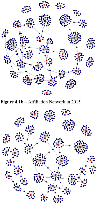
In the overall work, we are considering five main charts, and some key statistics about a fictious sixth one. The first step is the analysis of the affiliation networks, as a whole system of directors and companies, using a full bipartite graph without distinction in the different meaning and importance of the vertices (Figure 4.1); this is below referred to as the ‘full graph’, ‘bipartite graph’ or ‘overall graph’ from now onwards. At a first glance, the three graphs highlight a modest connectivity, and apparently none of the companies in the network appears to have a proper ‘central’ role; besides this, any analysis of indicators concerning two joint sets of vertices that we know having different roles and dignity could be misleading, and this is the reason why, despite being the chart carrying the biggest amount of information, we also use different representations that are derived from the same data.

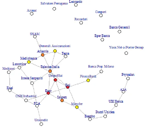
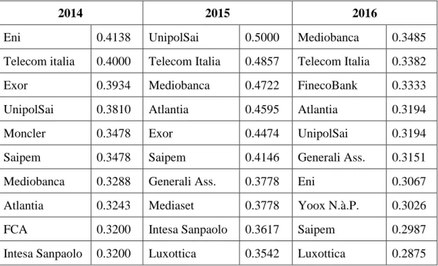
The second chart that we are considering is the induced graph (Figure 4.2) consisting of only the companies vertices (from now onwards, ‘companies network’), as it allows to gain insight into the connections of companies through the directors that the formers share; graphically speaking, this basically means that two companies are connected through an edge if there is at least a manager sitting on the boards of both. This chart plays a relevant role in the of the connections among companies as well as the clusters that form up, which are highlighted in the corresponding image as well. The same chart is also presented in a heatmap-like variant, for the purpose of analysing specifically the centrality of some of its elements and the behaviour of the core of the graph.

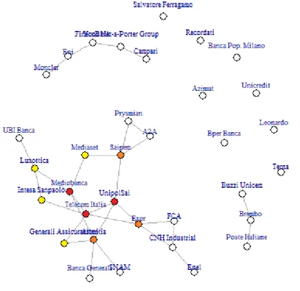
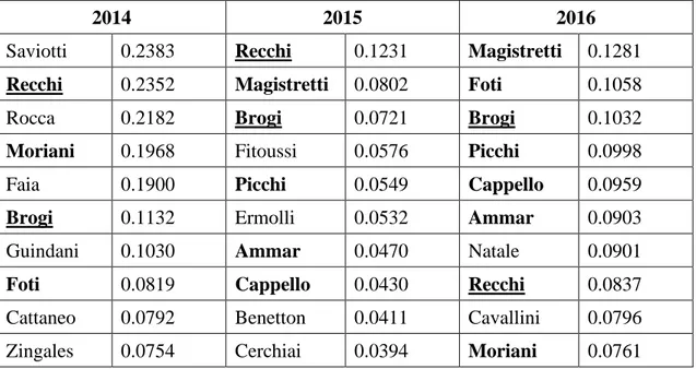
A third graph that deserves a special distinction in the analysis, especially in the identification of the most relevant key-players in the network, and is therefore sometimes mentioned, is a subgraph of the full bipartite graph including only the vertices of degree higher than 1 (Figure 4.3). The intent of this variation is to remove all the ‘noise’ of 1-degree directors that don’t create or shorten any connection between companies or people, being therefore of poor relevance for our purposes. Therefore, the graph includes all and only the ‘key directors’ whose removal from the network (i.e. they are fired) would imply the loss of a connection or, even worse, the complete detaching of a company from a cluster or a component. This helps detecting the parts of the charts that are most likely to be isolated and the key directors that keep them in the network. This representation may be referred to as ‘key-directors’, ‘key-players’ or ‘key-individuals’ graph.

30

As we are interested also in the dynamics inside the main component and less concerned about the companies that bring no connections or gather in isolated triples, two more interesting charts are a couple of subgraphs of the latter two (one for the companies chart, and one for the key-players chart) consisting only of the biggest component that is visible each year, i.e. the main components of the graphs present in Figure 4.1, 4.2 and 4.3.

Finally, some space in the analysis is dedicated to some features of a sixth chart, the induced graph of the directors alone, even if it is not graphically depicted because it would be hard to interpret.

4.3. LIMITS

Before proceeding through, one should be aware of the limits of this work, that may to a certain extent weaken or slightly bias the conclusions in this chapter, as well as in the followings.

Since the chart only includes 33 to 35 companies (the exact number depends on the year of observation), any consideration concerning its shape, density, centrality, connectivity, etc. could still be made without taking into account some important connections that are present outside of this framing and are beyond the scope of this study; the reasons of this issue emerging are mainly three: on the one hand, the fact that the subject of research is limited to listed Italian companies somewhat representative of the economy, further restricted because of the lack of availability of a minority of them; on the other hand, as non-listed companies are less subject to compliance and disclosure, it has been somewhat difficult to gather the data concerning their board composition on a regular yearly basis. For instance, the density values of the chart could be deemed surprisingly low (at least in absolute terms), albeit worth consideration; moreover, besides regulation issues, part of this evidence could be resulting from the restricted sample and the absence of extra-MIB connections, not mapped in the chart.

Furthermore, while still being valid and interesting for the analysis within the network, its representation may be part of a bigger framework that is not properly depicted in this context, meaning this could only be – and, very likely, is – the cohesive subset of vertices (or a subset of a cohesive partition) of a larger network, which is impossible to analyse both because of practical issues (the most important being gathering the data, especially concerning non-listed companies and other non-industrial entities such as clubs and institutions) and problems on a theoretical level (even if we

could gather the whole universe, its analysis would be messy and unclear as the set of data could be

32

5. A

FTSE-MIB

5.1. PRELIMINARY DESCRIPTIVE STATISTICS

Some initial analysis of the sample, disregarding the network and considering only the list of the companies, could provide some interesting insights concerning the composition of the sample, which is fully listed in the Table 5.1.

Some main features of this dataset can be highlighted on the spot, and they are all related to the peculiar structure of the Italian Economy: first, 33% of the companies in the sample offer some kind of banking, insurance or financial services, which is something that one would expect from a list of companies taken from an Italian market index; directly related to this point comes the second one: as per the art. 36 of the ‘Save Italy’ Law in 2011), most of the possible interlocking directorships within companies or groups operating in Banking, Insurance and Financial markets are forbidden; the implementation of this law, according to past literature, had an impact on the connectedness of the chart (Drago, Ricciuti, Santella, 2015); therefore, one could intuitively expect this to limit the connectivity within the network that is going to be analysed as well. Third, even when looking among the remaining companies, most of them (31%) operate within the same sectors: Fashion, Energy, Utilities. This could further lower the connectivity within the network, as there are very poor chances that a director, especially an insider or someone with an executive role, is found out ‘serving two masters’.

This preliminary analysis suggests a general lack of linkages between the companies, which should not be regarded with surprise, as it may have several other reasons, including the existence of connections outside FTSE-MIB companies, including non-listed firms or political institutions.

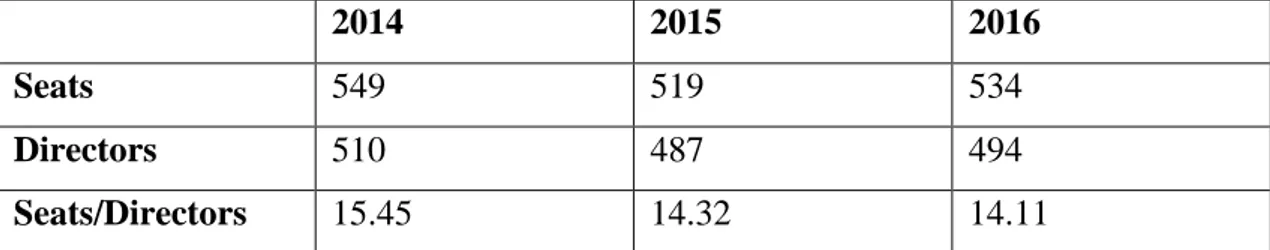
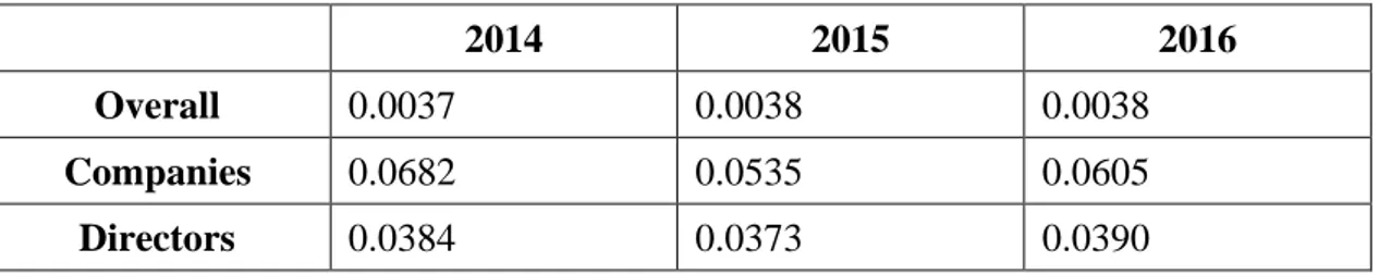
The widest representation of the network is the bipartite graph (Figure 4.1) consisting of the companies (33 to 35 from 2014 to 2016, respectively) present in the MIB in 2017 – net of the ones whose data is missing – and the corresponding directors (ranging from 487 to 494, depending on the year), for a total set of 543 elements (i.e., vertices) in 2014, 521 in 2015 and 529 in 2016, linked by a roughly equal amount of edges (respectively 549, 519, 534); all the relevant data are summarized in Table 5.2.

Despite the two sets of vertices are very different in the information they carry, a first glance analysis at the degree sequence (Table 5.3) is still feasible knowing that, given the nature of the dataset, all the vertices with degree ≤ 4 correspond to a director and the remaining ones are the

33

boards3. The degree of each of the vertices in these bigraphs has a notable meaning as it defines, depending on the nature of the vertex, either the number of the boards that a certain director sits on or the number of directors sitting on the boards of a certain company.

Concerning the directors (Table 5.3a), a vast majority of them (93.33% in 2014, 94.25% in 2015 and 92.91% in 2016) is only part of 1 board; this means that roughly, on average during the three years, all the connections among the companies – around 30 edges in the companies chart – are barely driven by the 6.5% of the directors.

Company-wise (Table 5.3b), the number of directors sitting on the boards ranges from 7 to 43 depending on the year and on the Company. Anyway, it is possible to notice a trend towards reduction of the directors in the boards (Table 5.4), with a median level dropping by 1 point per year and an average number of directors slowly diminishing as well4. This tendency towards a slight reduction in the number of board seats seems to be confirmed by the ratio between companies and number of directors (Table 5.5), i.e. the average number of directors per boards, which is 15.45 in 2014, 14.32 and 14.11 in 2016. The lower value of the simple ratio between directors and number of companies compared to the average grade of the companies themselves is imputable to their definition: by counting the degrees of each board, every director is technically counted multiple times, corresponding to the number of board seats they have, which is something that does not happen when one considers the overall number of directors, regardless of the number of boards they sit on. On the other hand, the relative closeness of these two set of numbers highlights a substantial lack of connections between directors.

The ratio related to the average board seats per director deserves a special mention; the value is 1.076 in 2014, 1.066 in 2015, 1.081 in 2016. The latter result can be seen as consistent with Elouaer’s (2009) analogous studies that show an average board membership per director in France5 equal to 1.19 / 1.22 in 2005 if one accepts the same conclusion as the author, who in particular highlights a decaying trend of the ratio, far higher in 1996 (1.33/1.30); assuming that the average board membership in Italy in the corresponding periods was roughly at least around the same scale, the decaying trend could explain the consequent drop to values that range from 1.066 to 1.081. To further strengthen both these two findings, the same indicator assumes a value of 1.12 in Germany in 2008 (Milaković, Alfarano, Lux, 2010). For the sake of completeness, one should also consider that at least 3 _{A manual check has been carried as well.}

4 _{Please notice that the 15.25 in 2016 is mainly due to the company with 43 degrees, which alone drives the average}

from 13.73 to 15.25 and the volatility from 4.13 to 7.49, while the highest degree observed in the companies of the other two subsets is 35

34

part of the cause of the slightly lower values for the Italian case may also be related to the lower number of companies considered compared to the German one, which leads to a higher likelihood of ignoring existing parallel board memberships of the directors in the sample, or to the peculiar structure of the Italian economy, where companies are most likely family-run with little participation of external share/stakeholders in the governance or in the property of the company.

5.2. NETWORK SHAPE, CLUSTERS AND EVOLUTION OVER TIME

A closer look at the set of linkages in the network, abstracting from metrics, could provide a more complete reference point in its description and in the analysis of its structure, in the sense that it can help to detect and explicitly mention the central companies and key directors that lead the connections, the tendency of the elements within the network to aggregate into clusters, and the evolution of such relationships over time.

As a reminder, we are considering two companies as ‘connected’ when they share at least one common director in their boards.

On the one hand, this analysis will focus on the clustered companies’ chart (Figure 4.2) and the ‘best partitions’ that it is possible to identify within it, albeit sometimes these may be very connected to each other. The exercise of shaping different subgraphs may prove particularly challenging as the graph becomes sparser and more decentralized or, at the extreme opposite, very compact. This is because, as mentioned above, a high level of flexibility is required when outlining the partitions and, in addition, sometimes using qualitative criterions could even be more complex than following some quantitative ‘decision boundary’. Therefore, while pursuing the goal of partitioning the entire chart, one has to accept that few partitions may be highly connected with some others or may include a huge number of vertices, giving unclear indications to interpret.

On the other hand, following the exactly opposite philosophy, a useful approach consists of simply isolating a subgraph of the formers, namely the largest component that shows up every time. Some of the considerations made can be, as a matter of fact, more trustworthy and effective once applied to this subset alone, because they focus more on the relationships, and sometimes give interesting explanations for counterintuitive evidence.

This two-level partitioning and analysis is the best compromise available to detect separate entities somewhat similar to clusters and keeping track of the most ‘critical’ links (we could say, the