UNIVERSITY
OF TRENTO
DEPARTMENT OF INFORMATION AND COMMUNICATION TECHNOLOGY
38050 Povo – Trento (Italy), Via Sommarive 14
http://www.dit.unitn.it
EFFICIENT INTERPOLANT GENERATION
IN SATISFIABILITY MODULO THEORIES
Alessandro Cimatti, Alberto Griggio, and Roberto Sebastiani
December 2007
Efficient Interpolant Generation
in Satisfiability Modulo Theories
⋆Alessandro Cimatti1, Alberto Griggio2, and Roberto Sebastiani2
1
FBK-IRST, Povo, Trento, Italy. [email protected]
2
DISI, Universit`a di Trento, Italy.{griggio,rseba}@disi.unitn.it
Abstract. The problem of computing Craig Interpolants for propositional (SAT) formulas has recently received a lot of interest, mainly for its applications in for-mal verification. However, propositional logic is often not expressive enough for representing many interesting verification problems, which can be more naturally addressed in the framework of Satisfiability Modulo Theories, SMT.
Although some works have addressed the topic of generating interpolants in SMT, the techniques and tools that are currently available have some limitations, and their performace still does not exploit the full power of current state-of-the-art SMT solvers.
In this paper we try to close this gap. We present several techniques for interpolant generation in SMT which overcome the limitations of the current generators men-tioned above, and which take full advantage of state-of-the-art SMT technology. These novel techniques can lead to substantial performance improvements wrt. the currently available tools.
We support our claims with an extensive experimental evaluation of our imple-mentation of the proposed techniques in the MathSAT SMT solver.
1
Introduction
Since the seminal paper of McMillan [18], interpolation has been recognized to be a substantial tool for verification in the case of boolean systems [7, 16, 17]. The tremen-dous improvements of Satisfiability Modulo Theory (SMT) solvers in the recent years have enabled the lifting of SAT-based verification algorithms to the non-boolean case [2, 1], and made it practical the implementation of other approaches such as CEGAR [20]. However, the research on interpolation for SMT has not kept the pace of the SMT solvers. In fact, the current approaches to producing interpolants for SMT [19, 29, 26, 15, 14] all suffer from a number of limitations. Some of the approaches are severely limited in terms of their expressiveness. For instance, the tool described in [26] can only deal with conjunctions of literals, whilst the recent work described in [15] can not deal with many useful theories. Furthermore, very few tools are available [26, 19], and these tools do not seem to scale particularly well. More than to na¨ıve implemen-tation, this appears to be due to the underlying algorithms, that substantially deviate from or ignore choices common in state-of-the-art SMT. For instance, in the domain
⋆
This work has been partly supported by ORCHID, a project sponsored by Provincia Autonoma di Trento, and by a grant from Intel Corporation.
of linear arithmetic over the rationals (LA(Q)), strict inequalities are encoded in [19] as the conjunction of a weak inequality and a disequality; although sound, this choice destroys the structure of the constraints, requires additional splitting, and ultimately re-sults in a larger search space. Similarly, the fragment of Difference Logic (DL(Q)) is dealt with by means of a general-purpose algorithm for fullLA(Q), rather than one of the well-known and much faster specialized algorithms. An even more fundamental example is the fact that state-of-the-art SMT reasoners use dedicated algorithms for Linear Arithmetic [9].
In this paper, we tackle the problem of generating interpolants within a state of the art SMT solver. We present a fully general approach that can generate interpolants for the most effective algorithms in SMT, most notably the algorithm for decidingLA(Q) presented in [9] and those forDL(Q) in [8, 22]. Our approach is also applicable to the combination of theories, based on the Delayed Theory Combination (DTC) method [5, 6], as an alternative to the traditional Nelson-Oppen method.
We carried out an extensive experimental evaluation on a wide range of benchmarks. The proposed techniques substantially advance the state of the art: our interpolator can deal with problems that can not be expressed in other solvers; furthermore, a compari-son on problems that can be dealt with by other tools shows dramatic improvements in performance, often by orders of magnitude.
The paper is structured as follows. In§2 we present some background on interpo-lation in SMT. In §3 and §4 we show how to efficiently interpolate LA(Q) and the subcase ofDL(Q). In §5 we discuss interpolation for combined theories. In §6 we an-alyze the experimental evaluation, whilst in§7 we draw some conclusions. The proofs of the theorems are reported in Appendix A.
2
Background
2.1 Satisfiability Modulo Theory – SMT
Our setting is standard first order logic. A0-ary function symbol is called a constant. A termis a first-order term built out of function symbols and variables. A linear term is either a linear combinationc1x1+ . . . + cnxn+ c, where c and ciare numeric constants andxi are variables. When doing arithmetic on terms, simplifications are performed where needed. We writet1 ≡ t2when the two termst1andt2are syntactically identi-cal. Ift1, . . . , tn are terms andp is a predicate symbol, then p(t1, . . . , tn) is an atom. A literal is either an atom or its negation. A (quantifier-free) formulaφ is an arbitrary boolean combination of atoms. We use the standard notions of theory, satisfiability, validity, logical consequence. We consider only theories with equality. We call Satis-fiability Modulo (the) TheoryT , SMT (T ), the problem of deciding the satisfiability of quantifier-free formulas wrt. a background theoryT .3
We denote formulas withφ, ψ, A, B, C, I, variables with x, y, z, and numeric con-stants witha, b, c, l, u. Given a theory T , we write φ |=T ψ (or simply φ |= ψ) to denote that the formulaψ is a logical consequence of φ in the theory T . With φ ¹ ψ we denote
3
The general definition of SMT deals also with quantified formulas. Nevertheless, in this paper we restrict our interest to quantifier-free formulas.
that all uninterpreted (inT ) symbols of φ appear in ψ. Without loss of generality, we also assume that the formulas are in Conjunctive Normal Form (CNF). IfC is a clause, C ↓ B is the clause obtained by removing all the literals whose atoms do not occur inB, and C \ B that obtained by removing all the literals whose atoms do occur in B. With a little abuse of notation, we might sometimes denote conjunctions of literals l1∧ . . . ∧ lnas sets{l1, . . . , ln} and vice versa. If η ≡ {l1, . . . , ln}, we might write ¬η to mean¬l1∨ . . . ∨ ¬ln.
We callT -solver a procedure that decides the consistency of a conjunction of literals inT . If S ≡ {l1, . . . , ln} is a set of literals in T , we call (T )-conflict set any subset η ofS which is inconsistent in T .4We call¬η a T -lemma (notice that ¬η is a T -valid clause). Given a set of clausesS ≡ {C1, . . . , Cn} and a clause C, we call a resolution proof thatV
iCi|=T C a DAG P such that:
1. C is the root of P;
2. the leaves ofP are either elements of S or T -lemmas;
3. each non-leaf nodeC′ has two parents Cp1 and Cp2 such thatCp1 ≡ p ∨ φ1,
Cp2 ≡ ¬p ∨ φ2, andC
′≡ φ
1∨ φ2. The atomp is called the pivot of Cp1andCp2.
IfC is the empty clause (denoted with ⊥), then P is a resolution proof of unsatisfiability forV
iCi.
A standard technique for solving the SMT(T ) problem is to integrate a DPLL-based SAT solver and aT -solver in a lazy manner (see, e.g., [27] for a detailed description). DPLL is used as an enumerator of truth assignments for the propositional abstraction of the input formula. At each step, the set ofT -literals S corresponding to the current as-signment is sent to theT -solver to be checked for consistency in T . If S is inconsistent, theT -solver returns a conflict set η, and the corresponding T -lemma ¬η is added as a blocking clause in DPLL, and used to drive the backjump mechanism. With a small modification of the embedded DPLL engine, a lazy SMT solver can also be used to generate a resolution proof of unsatisfiability.
2.2 Interpolation in SMT
We consider the SMT(T ) problem for some background theory T . Given an ordered pair(A, B) of formulas such that A ∧ B |=T ⊥, a Craig interpolant (simply “inter-polant” hereafter) is a formulaI s.t.:
a) A |=T I,
b) I ∧ B |=T ⊥,
c) I ¹ A and I ¹ B.
The use of interpolation in formal verification has been introduced by McMillan in [18] for purely-propositional formulas, and it was subsequently extended to han-dle SMT(EUF ∪ LA(Q)) formulas in [19], EUF being the theory of equality and uninterpreted functions. The technique is based on earlier work by Pudl´ak [24], where
4In the next sections, as we are in an SMT(T ) context, we often omit specifying “in the theory
two interpolant-generation algorithms are described: one for computing interpolants for propositional formulas from resolution proofs of unsatisfiability, and one for generating interpolants for conjunctions of (weak) linear inequalities inLA(Q). An interpolant for (A, B) is constructed from a resolution proof of unsatisfiability of A ∧ B, generated as outlined in§2.1. The algorithm can be described as follows:
Algorithm 1: Interpolant generation for SMT(T )
1. Generate a proof of unsatisfiabilityP for A ∧ B.
2. For everyT -lemma ¬η occurring in P, generate an interpolant I¬ηfor(η \ B, η ↓ B).
3. For every input clauseC in P, set IC≡ C ↓ B if C ∈ A, and IC ≡ ⊤ if C ∈ B.
4. For every inner nodeC of P obtained by resolution from C1 ≡ p ∨ φ1andC2≡ ¬p∨φ2, setIC≡ IC1∨IC2ifp does not occur in B, and IC≡ IC1∧IC2otherwise.
5. OutputI⊥as an interpolant for(A, B).
Notice that Step 2. of the algorithm is the only part which depends on the theory T , so that the problem of interpolant generation in SMT (T ) reduces to that of find-ing interpolants forT -lemmas. To this extent, in [19] McMillan gives a set of rules for constructing interpolants forT -lemmas in the theory of EUF, that of weak linear inequalities(0 ≤ t) in LA(Q), and their combination. Linear equalities (0 = t) can be reduced to conjunctions(0 ≤ t) ∧ (0 ≤ −t) of inequalities. Thanks to the combination of theories, also strict linear inequalities(0 < t) can be handled in EUF ∪ LA(Q) by replacing them with the conjunction(0 ≤ t) ∧ (0 6= t),5but this solution can be very inefficient. The combinationEUF ∪ LA(Q) can also be used to compute interpolants for other theories, such as those of lists, arrays, sets and multisets [14].
In [19], interpolants in the combined theoryEUF ∪LA(Q) are obtained by means of ad-hoc combination rules. The work in [29], instead, presents a method for generating interpolants for T1∪ T2 using the interpolant-generation procedures of T1 andT2as black-boxes, using the Nelson-Oppen approach [21].
Also the method of [26] allows to compute interpolants inEUF ∪ LA(Q). Its pecu-liarity is that it is not based on unsatisfiability proofs. Instead, it generates interpolants in LA(Q) by solving a system of constraints using an off-the-shelf Linear Programming (LP) solver. The method allows both weak and strict inequalities. Extension to unin-terpreted functions is achieved by means of reduction toLA(Q) using a hierarchical calculus. The algorithm works only with conjunctions of atoms, although in principle it could be integrated in Algorithm 1 to generate interpolants forT -lemmas in LA(Q). As an alternative, the authors show in [26] how to generate interpolants for formulas that are in Disjunctive Normal Form (DNF).
Another different approach is explored in [15]. There, the authors use the eager SMT approach to encode the original SMT problem into an equisatisfiable propositional problem, for which a propositional proof of unsatisfiability is generated. This proof is later “lifted” to the original theory, and used to generate an interpolant in a way similar to Algorithm 1. At the moment, the approach is however limited to the theory of equality only (without uninterpreted functions).
5
The details are not given in [19]. One possible way of doing this is to rewrite(0 6= t) as (y = t) ∧ (z = 0) ∧ (z 6= y), z and y being fresh variables.
HYP Γ ⊢ φφ∈ Γ LEQEQ Γ ⊢ 0 = t Γ ⊢ 0 ≤ t COMB Γ ⊢ 0 ≤ t1 Γ ⊢ 0 ≤ t2 Γ ⊢ 0 ≤ c1t1+ c2t2 c1, c2>0
Fig. 1. Proof rules forLA(Q) (without strict inequalities).
All the above techniques construct one interpolant for(A, B). In general, however, interpolants are not unique. In particular, some of them can be better than others, de-pending on the particular application domain. In [11], it is shown how to manipulate proofs in order to obtain stronger interpolants. In [12, 13], instead, a technique to re-strict the language used in interpolants is presented and shown to be useful in preventing divergence of techniques based on predicate abstraction.
3
Interpolation for Linear Arithmetic with a state-of-the-art solver
Traditionally, SMT solvers used some kind of incremental simplex algorithm [28] as T -solver for the LA(Q) theory. Recently, Dutertre and de Moura [9] have proposed a new simplex-based algorithm, specifically designed for integration in a lazy SMT solver. The algorithm is extremely efficient and was shown to significantly outperform (often by orders of magnitude) the traditional ones. It has now been integrated in several SMT solvers, including ARGOLIB, CVC3, MATHSAT, YICES, and Z3. Remarkably, this algorithm allows for handling also strict inequalities.In this Section, we show how to exploit this algorithm to efficiently generate inter-polants forLA(Q) formulas. In §3.1 we begin by considering the case in which the input atoms are only equalities and non-strict inequalities. In this case, we only need to show how to generate a proof of unsatisfiability, since then we can use the interpolation rules defined in [19]. Then, in§3.2 we show how to generate interpolants for problems containing also strict inequalities and disequalities.
3.1 Interpolation with non-strict inequalities
Similarly to [19], we use the proof rules of Figure 1: HYPfor introducing hypothe-ses, LEQEQfor deriving inequalities from equalities, and COMBfor performing linear combinations.6As in [19], we consider an atom “0 ≤ c”, c being a negative numerical constant, as a synonym of⊥.
The original de Moura algorithm. In its original formulation, the Dutertre-de Moura algorithm assumes that the variablesxi are partitioned a priori in two sets, hereafter denoted as ˆB (“initially basic”) and ˆN (“initially non-basic”), and that the algorithm receives as inputs two kinds of atomic formulas: 7
6In [19] the L
EQEQrule is not used inLA(Q), because the input is assumed to consist only of inequalities.
– a set of equations eqi, one for eachxi∈ ˆB, of the formPxj∈ ˆNˆaijxj+ ˆaiixi= 0
s.t. allaˆij’s are numerical constants;
– elementary atomsof the formxj ≥ ljorxj ≤ ujs.t.lj,ujare numerical constants. The initial equations eqiare then used to build a tableauT :
{xi =Pxj∈Naijxj| xi∈ B}, (1) whereB (“basic”), N (“non-basic”) and aij are such that initiallyB ≡ ˆB, N ≡ ˆN and aij ≡ −ˆaij/ˆaii.
In order to decide the satisfiability of the input problem, the algorithm performs manipulations of the tableau that change the sets B and N and the values of the co-efficientsaij, always keeping the tableauT in (1) equivalent to its initial version. An inconsistency is detected when it is not possible to satisfy all the bounds on the vari-ables introduced by the elementary atoms: as the algorithm ensures that the bounds on the variables inN are always satisfied, then there is a variable xi ∈ B such that the inconsistency is caused either by the elementary atomxi ≥ lior by the atomxi ≤ ui [9]. In the first case,8a conflict setη is generated as follows:
η = {xj≤ uj|xj ∈ N+} ∪ {xj ≥ lj|xj ∈ N−} ∪ {xi≥ li}, (2) wherexi =Pxj∈Naijxj is the row of the current version of the tableauT (1)
corre-sponding toxi,N+is{xj ∈ N |aij > 0} and N−is{xj ∈ N |aij < 0}. Notice that η is a conflict set in the sense that it is made inconsistent by (some of) the equations in the tableauT (1), i.e. T ∪ η |=LA(Q) ⊥.
In order to handle problems that are not in the above form, a satisfiability-preserving preprocessing step is applied upfront, before invoking the algorithm.
Our variant. In our variant of the algorithm, instead, the input is an arbitrary set of inequalitieslk ≤ Phˆakhyh oruk ≥ Phˆakhyh, and the preprocessing step is ap-plied internally. In particular, we introduce a “slack” variableskfor each distinct term P
hˆakhyhoccurring in the input inequalities. Then, we replace such term withsk(thus obtaininglk ≤ sk oruk ≥ sk) and add an equationsk =Phaˆkhyh. Notice that we introduce a slack variable even for “elementary” inequalities(lk ≤ yk). With this trans-formation, the initial tableauT (1) is:
{sk=Phˆakhyh}k, (3) s.t. ˆB is made of all the slack variables sk’s, ˆN is made of all the original variables yh’s, and the elementary atoms contain only slack variablessk’s.
In our variant, we can useη to generate a conflict set η′, thanks to the following lemma.
8Here we do not consider the second case x
Lemma 1. In the setη of (2), xiand all thexj’s are slack variables introduced by our preprocessing step. Moreover, the setη′ ≡ ηN+∪ ηN−∪ ηiis a conflict set, where
ηN+≡ {uk≥P
hˆakhyh|sk ≡ xjand xj∈ N+}, ηN− ≡ {lk≤Phˆakhyh|sk≡ xjand xj∈ N−},
ηi≡ {lk≤Phaˆkhyh|sk≡ xi}.
We construct a proof of inconsistency as follows. From the setη of (2) we build a conflict setη′by replacing each elementary atom in it with the corresponding original atom, as shown in Lemma 1. Using the HYPrule, we introduce all the atoms inηN+,
and combine them with repeated applications of the COMBrule: ifuk ≥Phˆakhyhis the atom corresponding tosk, we use as coefficient for the COMBtheaij (in thei-th row of the current tableau) such thatsk ≡ xj. Then, we introduce each of the atoms in ηN− with HYP, and add them to the previous combination, again using COMB. In this
case, the coefficient to use is−aij. Finally, we introduce the atom inηi and add it to the combination with coefficient1.
Lemma 2. The result of the linear combination described above is the atom0 ≤ c, such thatc is a numerical constant strictly lower than zero.
Besides the case just described (and its dual when the inconsistency is due to an elemen-tary atomxi ≤ ui), another case in which an inconsistency can be detected is when two contradictory atoms are asserted:lk≤Phˆakhyhanduk ≥Phˆakhyh, withlk> uk. In this case, the proof is simply the combination of the two atoms with coefficient 1.
The extension for handling also equalities likebk =Phˆakhyhis straightforward: we simply introduce two elementary atomsbk ≤ sk andbk ≥ sk and, in the construc-tion of the proof, we use the LEQEQrule to introduce the proper inequality.
Finally, notice that the current implementation in MATHSAT (see§6) is slightly different from what presented here, and significantly more efficient. In practice,η, η′ are not constructed in sequence; rather, they are built simultaneously. Moreover, some optimizations are applied to eliminate some slack variables when they are not needed. 3.2 Interpolation with strict inequalities and disequalities
Another benefit of the Dutertre-de Moura algorithm is that it can handle strict inequali-ties directly. Its method is based on the following lemma.
Lemma 3 (Lemma 1 in [9]). A set of linear arithmetic atomsΓ containing strict in-equalitiesS = {0 < p1, . . . , 0 < pn} is satisfiable iff there exists a rational number ε > 0 such that Γε= (Γ ∪ Sε) \ S is satisfiable, where Sε= {ε ≤ p1, . . . , ε ≤ pn}.
The idea of [9] is that of treating the infinitesimal parameterε symbolically instead of explicitly computing its value. Strict bounds(x < b) are replaced with weak ones (x ≤ b − ε), and the operations on bounds are adjusted to take ε into account.
We use the same idea also for computing interpolants. We transform every atom (0 < ti) occurring in the proof of unsatisfiability into (0 ≤ ti− ε). Then we compute an interpolantIεin the usual way. As a consequence of the rules of [19],Iεis always a single atom. As shown by the following lemma, ifIεcontainsε, then it must be in the form(0 ≤ t − c ε) with c > 0, and we can rewrite Iεinto(0 < t).
Lemma 4 (Interpolation with strict inequalities). LetΓ , S, Γεand Sε be defined as in Lemma 3. LetΓ be partitioned into A and B, and let Aε andBεbe obtained fromA and B by replacing atoms in S with the corresponding ones in Sε. LetIεbe an interpolant for(Aε, Bε). Then:
– Ifε 6¹ Iε, thenIεis an interpolant for(A, B).
– Ifε ¹ Iε, thenIε≡ (0 ≤ t−c ε) for some c > 0, and I ≡ (0 < t) is an interpolant for(A, B).
Thanks to Lemma 4, we can handle also negated equalities(0 6= t) directly. Suppose our setS of input atoms (partitioned into A and B) is the union of a set S′of equalities and inequalities (both weak and strict) and a setS6=of disequalities, and suppose that S′ is consistent. (If not so, an interpolant can be computed fromS′.) SinceLA(Q) is convex,S is inconsistent iff exists (0 6= t) ∈ S6=such thatS′∪{(0 6= t)} is inconsistent, that is, such that bothS′∪ {(0 < t)} and S′∪ {(0 > t)} are inconsistent.
Therefore, we pick one element(0 6= t) of S6=at a time, and check the satisfiability ofS′ ∪ {(0 < t)} and S′∪ {(0 > t)}. If both are inconsistent, from the two proofs we can generate two interpolants I− andI+. We combineI+ andI−
to obtain an interpolantI for (A, B): if (0 6= t) ∈ A, then I is I+∨ I−
; if(0 6= t) ∈ B, then I is I+∧ I−
, as shown by the following lemma.
Lemma 5 (Interpolation for negated equalities). LetA and B two conjunctions of LA(Q) atoms, and let n ≡ (0 6= t) be one such atom. Let g ≡ (0 < t) and l ≡ (0 > t). Ifn ∈ A, then let A+≡ A \ {n} ∪ {g}, A−≡ A \ {n} ∪ {l}, and B+≡ B−≡ B. Ifn ∈ B, then let A+≡ A−≡ A, B+≡ B \ {n} ∪ {g}, and B− ≡ B \ {n} ∪ {l}. Assume thatA+∧ B+ |=
LA(Q) ⊥ and that A−∧ B− |=LA(Q) ⊥, and let I+andI− be two interpolants for(A+, B+) and (A−, B−) respectively, and let
I ≡½ I
+∨ I−ifn ∈ A I+∧ I−ifn ∈ B. ThenI is an interpolant for (A, B).
4
Graph-based Interpolation for Difference Logic
Several interesting verification problems can be encoded using only a subset ofLA(Q), the theory of Difference Logic (DL(Q)), in which all atoms are inequalities of the form (0 ≤ y − x + c), where x and y are variables and c is a numerical constant. Equalities can be handled as conjunctions of inequalities. Here we do not consider the case when we also have strict inequalities(0 < y − x + c), because in DL(Q) they can be handled in a way which is similar to that described in§3.2 for LA(Q). Moreover, we believe that our method may be extended straightforwardly toDL(Z) because the graph-based algorithm described in this section applies also toDL(Z); in DL(Z) a strict inequality (0 < y −x +c) can be safely rewritten a priori into the inequality (0 ≤ y − x+c − 1).
DL(Q) is simpler than full linear arithmetic. Many SMT solvers use dedicated, graph-based algorithms for checking the consistency of a set ofDL(Q) atoms [8, 22].
Intuitively, a setS of DL(Q) atoms induces a graph whose vertexes are the variables of the atoms, and there exists an edgex −→ y for every (0 ≤ y − x + c) ∈ S. S isc inconsistent if and only if the induced graph has a cycle of negative weight.
We now extend the graph-based approach to generate interpolants. Consider the interpolation problem(A, B) where A and B are sets of inequalities as above, and let C be (the set of atoms in) a negative cycle in the graph corresponding to A ∪ B.
IfC ⊆ A, then A is inconsistent, in which case the interpolant is ⊥. Similarly, when C ⊆ B, the interpolant is ⊤. If neither of these occurs, then the edges in the cycle can be partitioned in subsets ofA and B. We call maximal A-paths of C a path x1
c1
−→ . . . cn−1
−−−→ xn such that (I)xi ci
−→ xi+1 ∈ A, and (II)C contains x′ c
′
−→ x1and xn
c′′
−→ x′′
that are inB. Clearly, the end-point variables x1, xnof the maximalA-path are suchx1, xn¹ A and x1, xn ¹ B.
Let the summary constraint of a maximalA-path x1 −→ . . .c1 cn−1
−−−→ xn be the in-equality0 ≤ xn−x1+Pn−1i=1 ci. We claim that the conjunction of summary constraints of theA-paths of C is an interpolant. In fact, using the rules for LA(Q) it is easy to see that a maximalA-path entails its summary constraint. Hence, A entails the conjunction of the summary constraints of maximalA-paths. Then, we notice that the conjunction of the summary constraints is inconsistent withB. In fact, the weight of a maximal A-path and the weight of its summary constraint are the same. Thus the cycle obtained fromC by replacing each maximalA-path with the corresponding summary constraint is also a negative cycle. Finally, we notice that every variablex occurring in the conjunction of the summary constraints is an end-point variable, and thusx ¹ A and x ¹ B.
A final remark is in order. In principle, to generate a proof of unsatisfiability for a conjunction ofDL(Q) atoms, the same rules used for LA(Q) [19] could be used. However, the interpolants generated from such proofs are in general notDL(Q) formu-las anymore and, if computed starting from the same inconsistent setC, they are either identical or weaker than those generated with our method. In fact, due to the interpola-tion rules in [19], it is easy to see that the interpolant obtained is in the form(0 ≤P
iti) s.t.V
i(0 ≤ ti) is the interpolant generated with our method.
Example 1. Consider the following sets ofDL(Q) atoms:
A = {(0 ≤ x1− x2+ 1), (0 ≤ x2− x3), (0 ≤ x4− x5− 1)} B = {(0 ≤ x5− x1), (0 ≤ x3− x4− 1)}. −1 −1 0 x1 x5 1 0 1 A B x2 x3 x4
corresponding to the negative cycle on the right. It is straightforward to see from the graph that the resulting interpolant is(0 ≤ x1− x3+ 1) ∧ (0 ≤ x4− x5− 1), because the first conjunct is the summary constraint of the first two conjuncts inA.
HYP (0 ≤ x1− x2+ 1) HYP (0 ≤ x2− x3) COMB (0 ≤ x1− x3+ 1) HYP (0 ≤ x4− x5− 1) COMB (0 ≤ x1− x3+ x4− x5) HYP (0 ≤ x5− x1) COMB (0 ≤ −x3+ x4) HYP (0 ≤ x3− x4− 1) COMB (0 ≤ −1)
By using the interpolation rules for LA(Q) (see [19]), the interpolant we obtain is (0 ≤ x1− x3+ x4− x5), which is not in DL(Q), and is weaker than that computed above.
5
Computing interpolants for combined theories via DTC
One of the typical approaches to the SMT problem in combined theories,SM T (T1∪ T2), is that of combining the solvers for T1and forT2with the Nelson-Oppen (NO) integration schema [21].
The NO framework works for combinations of stably-infinite and signature-disjoint theoriesTiwith equality. Moreover, it requires the input formula to be pure (i.e., s.t. all the atoms contain only symbols in one theory): if not, a purification step is performed, which might introduce some additional variables but preserves satisfiability. In this set-ting, the two decision procedures forT1andT2cooperate by exchanging (disjunctions of) implied interface equalities, that is, equalities between variables appearing in atoms of different theories (interface variables).
The work in [29] gives a method for generating an interpolant for a pair(A, B) of T1 ∪ T2-formulas using the NO schema. Besides the requirements onT1 andT2 needed to use NO, it requires also thatT1andT2are equality-interpolating. A theory T is said to be equality-interpolating when for all pairs of formulas (A, B) in T and for all equalities xa = xb such that (i) xa 6¹ B and xb 6¹ A (i.e. xa = xb is an AB-mixed equality), and (ii) A ∧ B |=T xa = xb, there exists a termt such that A ∧ B |=T xa = t ∧ t = xb,t ¹ A and t ¹ B. E.g., both EUF and LA(Q) are equality-interpolating.
Recently, an alternative approach for combining theories in SMT has been proposed, called Delayed Theory Combination (DTC) [5, 6]. With DTC, the solvers forT1and T2 do not communicate directly. The integration is performed by the SAT solver, by augmenting the boolean search space with up to all the possible interface equalities. DTC has several advantages wrt. NO, both in terms of ease of implementation and in reduction of search space [5, 6], so that many current SMT tools implement variants of DTC. In this Section, we give a method for generating interpolants for a pair ofT1∪ T2 -formulas(A, B) when T1andT2are combined using DTC. As in [29], we assume that A and B have been purified using disjoint sets of auxiliary variables.
5.1 Combination withoutAB-mixed interface equalities
LetEq be the set of all interface equalities introduced by DTC. We first consider the case in whichEq does not contain AB-mixed equalities. That is, Eq can be partitioned
into two sets(Eq \ B) ≡ {(x = y)|(x = y) ¹ A and (x = y) 6¹ B} and (Eq ↓ B) ≡ {(x = y)|(x = y) ¹ B}. In this restricted case, nothing special needs to be done, despite the fact that the interface equalities inEq do not occur neither in A nor inB, but might be introduced in the resolution proof P by T -lemmas. This is because —as observed in [19]— as long as for an atomp either p ¹ A or p ¹ B holds, it is possible to consider it part ofA (resp. of B) simply by assuming the tautology clause p ∨ ¬p to be part of A (resp. of B). Therefore, we can treat the interface equalities in (Eq \ B) as if they appeared in A, and those in (Eq ↓ B) as if they appeared in B.
5.2 Combination withAB-mixed interface equalities
We can handle the case in which some of the equalities inEq are AB-mixed under the hypothesis thatT1andT2are equality-interpolating. Currently, we also require thatT1 andT2 are convex, although the extension of the approach to non-convex theories is part of ongoing work.
The idea is similar to that used in [29] in the case of NO: using the fact that the Ti’s are equality-interpolating, we reduce this case to the previous one by “split-ting” everyAB-mixed interface equality (xa = xb) into the conjunction of two parts (xa = t) ∧ (t = xb), such that (xa= t) ¹ A and (t = xb) ¹ B. The main difference is that we do this a posteriori, after the construction of the resolution proof of unsatisfia-bilityP. This makes it possible to compute different interpolants for different partitions of the input problem into anA-part and a B-part from the same proof P. Besides the advantage in performance of not having to recompute the proof every time, this is par-ticularly important in some application domains like abstraction refinement [10], where the relation between interpolants obtained from the same proof tree is exploited to prove some properties of the refinement procedure.9 To do this, we traverseP and split every AB-mixed equality in it, performing also the necessary manipulations to ensure that the modified DAG is still a resolution proof of unsatisfiability (according to the definition in§2.2). As long as this requirement is met, our technique is independent from the exact procedure implementing it. In the rest of this Section, we describe the algorithm that we have implemented, for the combinationEUF ∪ LA(Q). Due to lack of space, we can not describe it in detail, rather we only provide the main intuitions.
First, we control the branching and learning heuristics of the SMT solver to ensure that the generated resolution proof of unsatisfiability P has a property that we call locality wrt. interface equalities. We say thatP is local wrt. interface equalities (ie -local) if the interface equalities occur only in subproofsPie
i ofP, in which both the root and the leaves areT1∪ T2-valid, the leaves ofPiieare also leaves ofP, the root of Piie does not contain any interface equality, and inPie
i all the pivots are interface equalities.
9
In particular, the following relation: IA,B∪C(P) ∧ C =⇒ IA∪C,B(P) (where IA,B(P) is
an interpolant for(A, B) generated from the proof P) is used to show that for every spurious counterexample found, the interpolation-based refinement procedure is able to rule-out the counterexample in the refined abstraction [10]. It is possible to show that a similar relation holds also for IA,B∪C(P1) and IA∪C,B(P2), when P1 andP2are obtained from the same
P by splitting AB-mixed interface equalities with the technique described here. However, for lack of space we can not include such proof.
In order to generate ie -local proofs, we adopt a variant of the DTC Strategy 1 of [6]. We never select an interface equality for case splitting if there is some other unassigned atom, and we always assign false to interface equalities first. Moreover, when splitting on interface equalities, we restrict both the backjumping and the learning procedures of the DPLL engine as follows. Letd be the depth in the DPLL tree at which the first interface equality is selected for case splitting. If during the exploration of the current DPLL branch we have to backjump aboved, then we generate by resolution a conflict clause that does not contain any interface equality, and “deactivate” all theT -lemmas containing some interface equality, so that they can not be used elsewhere in the search tree. Only when we start splitting on interface equalities again, we can re-activate such T -lemmas.
The idea of the Strategy just described is that of “emulating” the NO combination of the twoTi-solvers. The conflict clause generated by resolution plays the role of the T -lemma generated by the NO-based T1∪ T2 solver, and the T -lemmas containing positive interface equalities are used for exchanging implied equalities. The difference is that the combination is performed by the DPLL engine, and encoded directly in the ie -local subproofsPie
i ofP.
SinceAB-mixed equalities can only occur in Pie
i subproofs, we can handle the rest ofP in the usual way. Therefore, we now describe only how to manipulate the Pie
i ’s such that all theAB-mixed equalities are split.
In order accomplish this task, we exploit the following fact: since we are considering only convex theories, all theTi-lemmas generated by theTi-solvers contain at most one positive interface equality(x = y).10
LetC ≡ (x = y) ∨ ¬η be one such Ti-lemma. Thenη |=Ti (x = y). Since Tiis equality-interpolating, if(x = y) is AB-mixed, we
can splitC into C1 ≡ (x = t) ∨ ¬η and C2 ≡ (t = y) ∨ ¬η. (E.g. by using the algorithms given in [29] forEUF and LA(Q).) Then, we replace every occurrence of ¬(x = y) in the leaves of Pie
i with the disjunction¬(x = t) ∨ ¬(t = y). Finally, we replace the subproof
(x = y) ∨ ¬η ¬(x = y) ∨ φ
¬η ∨ φ with
(x = t) ∨ ¬η ¬(x = t) ∨ ¬(t = y) ∨ φ
¬η ∨ ¬(t = y) ∨ φ (t = y) ∨ ¬η
¬η ∨ φ .
If this is done recursively, starting fromTi-lemmas¬η ∨ (x = y) such that ¬η contains no negatedAB-mixed equality, then the procedure terminates and the new proof Pie
i ′ contains noAB-mixed equality.
Finally, we wish to remark that what just described is only one possible way of splittingAB-mixed equalities in P. In particular, the restrictions on the branching and learning heuristics needed to generate ie -local proofs might have a negative impact in the performance of the SMT solver. In fact, we are currently investigating some alternative strategies.
10
There is a further technical condition that must be satisfied by theTi-solvers, i.e. they must not
generate conflict sets containing redundant disequalities. This is true for all theTi-solvers on
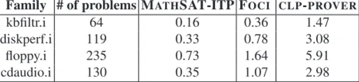
Family # of problems MATHSAT-ITP FOCI CLP-PROVER
kbfiltr.i 64 0.16 0.36 1.47 diskperf.i 119 0.33 0.78 3.08 floppy.i 235 0.73 1.64 5.91 cdaudio.i 130 0.35 1.07 2.98
Fig. 2. Comparison of execution times of MATHSAT-ITP, FOCIandCLP-PROVERon problems generated by BLAST.
6
Experimental evaluation
The techniques presented in previous sections have been implemented within MATH -SAT 4 [4] (Hereafter, we will refer to such implementation as MATHSAT-ITP). MATH -SAT is an SMT solver supporting a wide range of theories and their combinations. In the last SMT solvers competition (SMT-COMP’07), it has proved to be competitive with the other state-of-the-art solvers. In this Section, we experimentally evaluate our approach.
6.1 Description of the benchmark sets
We have performed our experiments on two different sets of benchmarks. The first is obtained by running the BLAST software model checker [10] on some Windows device drivers; these are similar to those used in [26]. This is one of the most important applications of interpolation in formal verification, namely abstraction refinement in the context of CEGAR. The problem represents an abstract counterexample trace, and consists of a conjunction of atoms. In this setting, the interpolant generator is called very frequently, each time with a relatively simple input problem.
The second set of benchmarks originates from the SMT-LIB [25], and is composed of a subset of the unsatisfiable problems used in the 2007 SMT solvers competition (http://www.smtcomp.org). The instances have been converted to CNF and then split in two consistent parts of approximately the same size. The set consists of problems of varying difficulty and with a nontrivial boolean structure.
The experiments have been performed on a 3GHz Intel Xeon machine with 4GB of RAM running Linux. All the tools were run with a timeout of 600 seconds and a memory limit of 900 MB.
6.2 Comparison with the state-of-the-art tools available
In this section, we compare with the only other interpolant generators which are avail-able: FOCI [19, 12] and CLP-PROVER [26]. Other natural candidates for comparison would have been ZAP[3] and LIFTER[15]; however, it was not possible to obtain them from the authors.
The comparison had to be adapted to the limitations of FOCIandCLP-PROVER. In
Execution Time Size of the Interpolant F O C I 0.1 1 10 100 1000 0.1 1 10 100 1000 2x 4x Single theory Multiple theories 10 100 1000 10000 100000 1e+06 10 100 1000 10000 100000 1e+06 2x 4x Single theory Multiple theories
MATHSAT-ITP MATHSAT-ITP Fig. 3. Comparison of MATHSAT-ITP and FOCIon SMT-LIB instances: execution time (left), and size of the interpolant (right). In the left plot, points on the horizontal and vertical lines are timeouts/failures.
Execution Time C L P -P R O V E R 0.01 0.1 1 10 100 1000 0.01 0.1 1 10 100 1000 2x 4x MATHSAT-ITP Fig. 4. Comparison of MATH -SAT-ITP and CLP-PROVER
on conjunctions of LA(Q) atoms.
fragment11. We also notice that the interpolants it generates are not always DL(Q) formulas. (See, e.g., Example 1 of Section 4.)CLP-PROVER, on the other hand, does handle the fullLA(Q), but it accepts only conjunctions of atoms, rather than formulas with arbitrary boolean structure. These limitations made it impossible to compare all the three tools on all the instances of our benchmark sets. Therefore, we perform the following comparisons:
– We compare all the three solvers on the problems generated by BLAST;
– We compare MATHSAT-ITP with FOCIon SMT-LIB instances in the theories of EUF, DL(Q) and their combination. In this case, we compare both the execution times and the sizes of the generated interpolants (in terms of number of nodes in the DAG representation of the formula). For computing interpolants inEUF, we apply the algorithm of [19], using an extension of the algorithm of [23] to generate EUF proof trees. The combination EUF ∪ DL(Q) is handled with the technique described in§5;
– We compare MATHSAT-ITP andCLP-PROVERonLA(Q) problems consisting of conjunctions of atoms. These problems are single branches of the search trees ex-plored by MATHSAT for someLA(Q) instances in the SMT-LIB. We have
col-lected several problems that took more than0.1 seconds to MATHSAT to solve, and then randomly picked50 of them. In this case, we do not compare the sizes of the interpolants as they are always atomic formulas.
The results are collected in Figures 2, 3 and 4. We can observe the following facts:
– Interpolation problems generated by BLASTare trivial for all the tools. In fact, we even had some difficulties in measuring the execution times reliably. Despite this, MATHSAT-ITP seems to be a little faster than the others.
11
For example, it fails to detect the LA(Q)-unsatisfiability of the following problem: (0 ≤ y− x + w) ∧ (0 ≤ x − z − w) ∧ (0 ≤ z − y − 1) .
– For problems with a nontrivial boolean structure, MATHSAT-ITP outperforms FOCI
in terms of execution time. This is true even for problems in the combined theory EUF ∪ DL(Q), despite the fact that the current implementation is still preliminary.
– In terms of size of the generated interpolants, the gap between MATHSAT-ITP and
FOCIis smaller on average. However, the right plot of Figure 3 (which considers only instances for which both tools were able to generate an interpolant) shows that there are more cases in which MATHSAT-ITP produces a smaller interpolant.
– On conjunctions ofLA(Q) atoms, MATHSAT-ITP outperformsCLP-PROVER, some-times by more than two orders of magnitude.
7
Conclusions
In this paper, we have shown how to efficiently build interpolants using state-of-the-art SMT solvers. Our methods encompass a wide range of theories (includingEUF, difference logic, and linear arithmetic), and their combination (based on the Delayed Theory Combination schema). A thorough experimental evaluation shows that the pro-posed methods are vastly superior to the state of the art interpolants, both in terms of expressiveness, and in terms of efficiency.
In the future, we plan to investigate the following issues. First, we will improve the implementation of the interpolation method for combined theories, that is currently rather na¨ıve, and limited to the case of convex theories. Second, we will investigate interpolation with other rules, in particular Ackermann’s expansion. Finally, we will integrate our interpolator within a CEGAR loop based on decision procedures, such as BLAST or the new version of NuSMV. In fact, such an integration raises interesting problems related to controlling the structure of the generated interpolants [12, 13], e.g. in order to limit the number or the size of constants occurring in the proof.
References
1. G. Audemard, M. Bozzano, A. Cimatti, and R. Sebastiani. Verifying industrial hybrid sys-tems with mathsat. Electr. Notes Theor. Comput. Sci., 119(2), 2005.
2. G. Audemard, A. Cimatti, A. Kornilowicz, and R. Sebastiani. Bounded model checking for timed systems. In Proc. FORTE, volume 2529 of LNCS. Springer, 2002.
3. T. Ball, S. K. Lahiri, and M. Musuvathi. Zap: Automated theorem proving for software analysis. In Proc. LPAR, volume 3835 of LNCS. Springer, 2005.
4. M. Bozzano, R. Bruttomesso, A. Cimatti, T. Junttila, P. Rossum, S. Schulz, and R. Sebastiani. MathSAT: A Tight Integration of SAT and Mathematical Decision Procedure. Journal of Automated Reasoning, 35(1-3), October 2005.
5. M. Bozzano, R. Bruttomesso, A. Cimatti, T. Junttila, P. van Rossum, S. Ranise, and R. Se-bastiani. Efficient Theory Combination via Boolean Search. Information and Computation, 204(10), 2006.
6. R. Bruttomesso, A. Cimatti, A. Franz´en, A. Griggio, and R. Sebastiani. Delayed Theory Combination vs. Nelson-Oppen for Satisfiability Modulo Theories: A Comparative Analysis. In Proc. LPAR, volume 4246 of LNCS. Springer, 2006.
7. G. Cabodi, M. Murciano, S. Nocco, and S. Quer. Stepping forward with interpolants in unbounded model checking. In Proc. ICCAD’06,. ACM, 2006.
8. S. Cotton and O. Maler. Fast and Flexible Difference Constraint Propagation for DPLL(T). In Proc. SAT, volume 4121 of LNCS. Springer, 2006.
9. B. Dutertre and L. de Moura. A Fast Linear-Arithmetic Solver for DPLL(T). In Proc .CAV, volume 4144 of LNCS, 2006.
10. T. A. Henzinger, R. Jhala, R. Majumdar, and K. L. McMillan. Abstractions from proofs. In N. D. Jones and X. Leroy, editors, POPL. ACM, 2004.
11. R. Jhala and K. McMillan. Interpolant-based transition relation approximation. In Proc. CAV, volume 3576 of LNCS. Springer, 2005.
12. R. Jhala and K. L. McMillan. A Practical and Complete Approach to Predicate Refinement. In H. Hermanns and J. Palsberg, editors, TACAS, volume 3920 of LNCS. Springer, 2006.
13. R. Jhala and K. L. McMillan. Array Abstractions from Proofs. In W. Damm and H. Her-manns, editors, CAV, volume 4590 of LNCS. Springer, 2007.
14. D. Kapur, R. Majumdar, and C. G. Zarba. Interpolation for data structures. In M. Young and P. T. Devanbu, editors, SIGSOFT FSE. ACM, 2006.
15. D. Kroening and G. Weissenbacher. Lifting Propositional Interpolants to the Word-Level. In FMCAD, pages 85–89, Los Alamitos, CA, USA, 2007. IEEE Computer Society.
16. B. Li and F. Somenzi. Efficient Abstraction Refinement in Interpolation-Based Unbounded Model Checking. In Proc. TACAS, volume 3920 of LNCS. Springer, 2006.
17. J. Marques-Silva. Interpolant Learning and Reuse in SAT-Based Model Checking. Electr. Notes Theor. Comput. Sci., 174(3):31–43, 2007.
18. K. McMillan. Interpolation and SAT-based model checking. In Proc. CAV, 2003.
19. K. L. McMillan. An interpolating theorem prover. Theor. Comput. Sci., 345(1), 2005.
20. K. L. McMillan. Lazy Abstraction with Interpolants. In Proc CAV, volume 4144 of LNCS. Springer, 2006.
21. G. Nelson and D. Oppen. Simplification by Cooperating Decision Procedures. ACM Trans. on Programming Languages and Systems, 1(2), 1979.
22. R. Nieuwenhuis and A. Oliveras. DPLL(T) with Exhaustive Theory Propagation and Its Application to Difference Logic. In Proc. CAV, volume 3576 of LNCS. Springer, 2005.
23. R. Nieuwenhuis and A. Oliveras. Fast Congruence Closure and Extensions. Inf. Comput., 2005(4):557–580, 2007.
24. P. Pudl´ak. Lower bounds for resolution and cutting planes proofs and monotone computa-tions. J. of Symb. Logic, 62(3), 1997.
25. S. Ranise and C. Tinelli. The Satisfiability Modulo Theories Library (SMT-LIB). www.SMT-LIB.org, 2006.
26. A. Rybalchenko and V. Sofronie-Stokkermans. Constraint Solving for Interpolation. In VMCAI, LNCS. Springer, 2007.
27. R. Sebastiani. Lazy Satisfiability Modulo Theories. Journal on Satisfiability, Boolean Mod-eling and Computation, JSAT, Volume 3, 2007.
28. R. J. Vanderbei. Linear Programming: Foundations and Extensions. Springer, 2001.
29. G. Yorsh and M. Musuvathi. A combination method for generating interpolants. In R. Nieuwenhuis, editor, CADE, volume 3632 of LNCS. Springer, 2005.
A
Appendix: Proofs
A.1 Proof of Lemma 1Proof. In order to prove the lemma, we need to give some details on how the Dutertre-de Moura algorithm Dutertre-detects an inconsistency. The algorithm maintains a mappingβ : B ∪ N 7−→ Q representing a candidate model which, at every step, satisfies the follow-ing invariants:
∀xj∈ N , lj≤ β(xj) ≤ uj, ∀xi∈ B, β(xi) =Pj∈Naijβ(xj). (4) The algorithm tries to adjust the values of β and the sets B and N , and hence the coefficientsaij of the tableau, such thatli ≤ β(xi) ≤ ui holds also for all thexi’s in B. Inconsistency is detected when this is not possible without violating any constraint in (4).
We consider the case in whichη (2) is generated from a row xi=Pxj∈Naijxjin
the tableauT (1) such that β(xi) < li. In [9] it is shown that in this case the following facts hold:
∀xj∈ N+, β(xj) = uj, and ∀xj∈ N−, β(xj) = lj. (5) (We recall that N+ = {x
j ∈ N |aij > 0} and N− = {xj ∈ N |aij < 0}.) The bounds uj andlj can be introduced only by elementary atoms. Since in our variant the elementary atoms contain only slack variables, eachxj must be a slack variable (namelysk). The same holds forxi(since its value is bounded byli).
Now considerη again. In [9] it is shown that when a conflict is detected because β(xi) < li, then the following fact holds:
β(xi) =Pxj∈N+aijuj+
P
xj∈N−aijlj. (6)
From thei-th row of the tableau T (1) we can derive 0 ≤P
xj∈Naijxj− xi. (7)
If we take each inequality0 ≤ uj−xjmultiplied by the coefficientaijfor allxj ∈ N+, each inequality0 ≤ xj − lj multiplied by coefficient−aij for allxj ∈ N−, and the inequality(0 ≤ xi− li) multiplied by 1, and we add them to (7), we obtain
0 ≤P
N+aijuj+PN−aijlj− li, (8) which by (6) is equivalent to 0 ≤ β(xi) − li. Thus we have obtained 0 ≤ c with c ≡ β(xi) − li, which is strictly lower than zero. Therefore,η is inconsistent under the definitions inT . Since we know that xiand all thexj’s inη are slack variables, we can replace everyxj(i.e., everysk) with its corresponding termPhˆakhyh, thus obtaining
η′, which is thus inconsistent. ⊓⊔
A.2 Proof of Lemma 2
A.3 Proof of Lemma 4
Proof. Since the side condition of the COMBrule ensures that equations are combined only using positive coefficients, and since the atoms introduced in the proof either do not containε or contain it with a negative coefficient, if ε appears in Iε, it must have a negative coefficient.
Ifε does not appear in Iε, thenIεhas been obtained from atoms appearing inA or B, so that Iεis an interpolant for(A, B).
Ifε appears in Iε, since its value has not been explicitly computed, it can be arbitrar-ily small, so thanks to Lemma 3 we have thatBε∧Iε|=LA(Q)⊥ implies B ∧I |=LA(Q) ⊥.
We can prove thatA |=LA(Q)I as follows. We consider some interpretation µ which is a model forA. Since ε does not occur in A, we can extend µ by setting µ(ε) = δ for someδ > 0 such that µ is a model also for Aε. AsAǫ|=LA(Q) Iǫ,µ is also a model for Iε, and henceµ is also a model for I. Thus, we have that A |=LA(Q) I. ⊓⊔ A.4 Proof of Lemma 5
Proof. We have to prove that:
a) A |=LA(Q)I
b) B ∧ I |=LA(Q)⊥
c) I ¹ A and I ¹ B.
a) Ifn ∈ A, then A |=LA(Q) g ∨ l. By hypothesis, we know that A+ |=LA(Q) I+ andA− |=
LA(Q) I−. Then trivially A ∪ {g} |=LA(Q) I+ andA ∪ {l} |=LA(Q) I−. ThereforeA ∪ {g} |=
LA(Q) I+∨ I− andA ∪ {l} |=LA(Q) I− ∨ I+, so that A |=LA(Q)I.
Ifn ∈ B, then A+ ≡ A− ≡ A. By hypothesis A |=
LA(Q) I+andA |=LA(Q) I−, so thatA |=LA(Q)I.
b) If n ∈ A, then B+ ≡ B− ≡ B. By hypothesis B ∧ I+ |=
LA(Q) ⊥ and B ∧ I−|=LA(Q) ⊥, so that B ∧ I |=LA(Q)⊥.
Ifn ∈ B, then B |=LA(Q) g ∨ l, so that either B → g or B → l must hold. By hypothesis we haveB+∧I+|=
LA(Q)⊥, so that B ∪{g}∧I+|=LA(Q)⊥. If B → g holds, thenB ∧ I+ |=LA(Q) ⊥, and hence B ∧ I |=LA(Q) ⊥. Similarly, if B → l holds, thenB ∧ I−|=
LA(Q) ⊥, and so again B ∧ I |=LA(Q)⊥.
c) By the hypothesis, bothI+andI− contain only symbols common toA and B, so