International equity markets interdependence: bigger shocks or contagion in the 21st century?

International Equity Markets Interdependence:

Bigger Shocks or Contagion in the 21st Century?

Giovanna Bua

 

Central Bank of Ireland

Carmine Trecroci

1



University of Brescia

This draft: 13 June 2018

Abstract

We investigate the nature of shocks across international equity markets and evaluate the shifts in their comovements at a business-cycle frequency. By using a parsimonious “identification through heteroskedasticity” methodology, we compute the impact exposures of index returns to common and country-specific shocks. We then establish some key results regarding comovement amongst international returns and macroeconomic fluctuations over the last decades. First, across all indices, persistent high-volatility, high cross-market correlation spells always coincide with macroeconomic slowdowns, and they coincide with measured shifts in macroeconomic and financial uncertainty. Second, there is a rise in the observed responses of international stock returns to common shocks during turbulent periods; such increase is largely attributable to bigger shocks (heteroskedasticity of fundamentals) rather than to breaks in the transmission mechanism or increased structural interdependence between markets. This holds for the Great Financial Crisis too. Third, since around the turn of the millennium, returns have experienced more often high volatility and comovement, likely because of larger and persistent macroeconomic disturbances.

Keywords: International equity markets; Volatility; Regime switching; Structural transmission. JEL Codes: C32, C51, G15.

1 _{Corresponding author. Department of Economics and Management, University of Brescia, Via San Faustino 74/B,}

25122 Brescia, carmine.trecroci@unibs.it. We are grateful to José Eduardo Gómez González, Anton Muscatelli, Franco Spinelli, Pietro Veronesi, two anonymous referees and seminar participants at the University of Brescia, Bank of Italy and Infiniti 2017 Conference for very helpful comments. All errors remain ours.

1 Introduction

Asset prices and aggregate economic fluctuations are related. A key insight of empirical finance is that equity market’s willingness to take risk varies over time: higher in good times, lower in bad times. As a consequence, market returns tend to be serially correlated and heteroskedastic. More precisely, returns display recurrent and sometimes prolonged spells of high volatility. The market prices of risk vary over time and, because of their adjustment to new information, induce time variation in the volatility of returns. Several studies document that the variability of returns tends to be higher during downside, or “bear” markets, than during upside or “bull” markets. A closely associated phenomenon regards market correlations: they too seem to vary over time and to rise around episodes of financial distress. Research has labelled those instances as contagion, i.e., fast and sustained propagation of shocks from their epicenter towards other financial markets (see King and Wadhwani, 1990; Lee and Kim, 1993; Kaminsky et al., 2003; Pericoli and Sbracia, 2003).

One case particularly relevant because of its implications for portfolio choices and macroeconomic policies is that of lower-frequency comovements between international equity market indices. Since Kaminsky et al. (2003) contagion is being studied as “...an episode in which there are significant immediate effects in a number of countries following an event—that is, when the consequences are fast and furious and evolve over a matter of hours or days”. However, over the past decades we have observed several episodes of sustained international comovement of asset markets that have contagion-like properties, like being unanticipated by markets, but they are also more persistent and interplay more clearly with macroeconomic and financial variables. This paper identifies shocks across international stock markets and empirically evaluates the nature of shifts in their comovements. Our analysis departs from most existing studies as we choose a combination of methodology and data that focuses on the relationship of international equity markets interdependence with business cycle developments.

Figure 1 provides some background to our investigation. It shows the cross-country average correlation of monthly returns of six advanced-economy equity markets (USA, Japan, UK, France, Germany, Canada) with an equally-weighted global index.2_{The correlations are computed between 1970 and early}

2016 on a 30-month rolling window. The black marks on the x-axis denote periods during which weighted real GDP growth (computed with respect to the same quarter of the previous year) in the six countries was below 1%, whereas the shaded areas indicate NBER-dated recessions in the US. The GDP data show a remarkable synchronization of macroeconomic slowdowns between the US and the other countries. However, the correlations point to further regularities, particularly valuable given the monthly frequency of our data. First, international equity correlations display a clear tendency to grow and remain high around notable episodes of financial turbulence, such as 1987, 1997-1998, 2000-2002 and 2008 to 2010. Second, macroeconomic downturns too tend to accompany increases in correlations, and US recessions always lead slowdowns in the rest of the countries. In those instances, international markets seem to move more closely with the US.3 _{Third, correlations have climbed up from around 0.65 in the late 1990s and since the Great}

2 _{Very similar dynamics shows up when using a value-weighted index such as the MSCI World.} 3 _{See Baele and Inghelbrecht (2009), Bekaert et al. (2014) and Pukthuanthong and Roll (2009).}

Financial Crisis appear to have plateaued at a permanently higher level close to 0.9 (see also Morana and Beltratti, 2008).

These facts seemingly point to some structural change having occurred after 1995, either in the transmission or in the origination of shocks. However, sharp conclusions from simple correlation coefficients would be misleading. In the context of a risk factor model, it is straightforward to show that correlations increase with betas and factor volatilities and decrease with idiosyncratic volatility, everything else being equal. In addition, past studies claimed (see Schwert, 1989a, b, for instance) that market volatility, while varying over time, shows no long-term trend. Therefore, the dynamics of simple measures of comovement such as correlations could either be driven by changes in the size of shocks, or be the result of structural shifts in the sensitivity of returns to systematic disturbances with macroeconomic and financial origins.4

We employ a parsimonious approach to identify the regime shifts in the comovement across equity indices at business-cycle frequency. The key question is: Are comovements indeed caused by changes in the transmission of shocks hitting the markets, or rather the outcome of changing volatility? The answer to this question has important implications for both theoretical and empirical models of interdependence, for investors as well as in the design of policies aiming to dampen the undesirable effects of volatility and comovement.

FIGURE 1 HERE

Figure 1. Conditional average correlation across stock market returns

The line represents the cross-market average of the 30-month rolling correlations of each country index with an equally-weighted index of the stock market returns across the US, Japan, UK, France, Germany, Canada. Lower black marks denote periods during which the weighted average of the quarterly GDP growth rate, compared to the same quarter of the previous year and seasonally adjusted, was below 1%; shaded bars indicate NBER-dated recessions of the US economy.

This paper extends the methodology first employed by Gravelle, Kirchian and Morley (2006) and then, amongst others, by Flavin et al. (2008, 2009) and Lagoarde-Segot and Lucey (2009). Contagion implies an association between markets beyond what one would expect from economic fundamentals. However, most studies focus on bilateral models estimated on data at the daily or weekly frequency, thus making it hard to capture the exact nature of their interplay with business cycle developments, to which we are primarily interested. Accordingly, and in contrast with existing studies, our specification centers on one-factor models for international stock market indices, where the factor is represented by the return on a well-diversified basket of international stocks, and we use monthly data over 1970-2016. Because of these modelling choices, our conditional loadings capture the exposures of returns to common and country-specific shocks, are exempt from short-term market noises and are likely to respond only to persistent changes in the information set of investors. The parameters governing the transmission of shocks across markets are identified assuming that the volatility of shocks experiences regime shifts. However, again in contrast with most of the extant literature, our approach allows for the timing of changes in comovement and volatility to be fully endogenous. We posit that a latent variable (the ‘state’ of the economy) determines both the mean of output

growth and the scale of stock return variances and covariances. This latent variable takes on one of an infinite set of values and is presumed to be determined by an unobserved Markov chain. This way, the probability of returns switching from a regime of volatility and comovement to another, rather than constant, is assumed dependent on uncertainty about underlying macroeconomic fundamentals.

We hypothesize that systematic and return-specific disturbances switch between low-volatility and high-volatility states. The intuition that we exploit for the returns on any two indices is consistent with the definitions of contagion (‘excess’ or ‘increased’ interdependence, or ‘shift-contagion’) by Kaminsky et al. (2003) and Pericoli and Sbracia (2003). In the baseline scenario (normal interdependence), an increase in the comovement between index returns could just reflect larger common shocks, hitting through invariant structural linkages. If this were the case, the coefficients linking the unexpected components of the two returns to the common shocks would both be larger during bad times or financial distress. We evaluate the interdependence between index returns by studying the ratio of the impact coefficients on the common shocks. Hence, in ‘tranquil’ circumstances, they would both increase proportionally to the size of the common shocks, leaving their ratio approximately equal to its normal-times value. By contrast, financial market distress or a shift in underlying economic fundamentals might produce a break in the transmission of systematic shocks to the two returns. This would be a scenario of increased structural interdependence, or ‘slower-moving contagion’ and the ratio of impact coefficients would turn out to be higher during bad times than under normal times. We therefore exploit this intuition to test for contagion (i.e., increased structural interdependence, see the taxonomy proposed in Pericoli and Sbracia, 2003) through the analysis of impact coefficients for the systematic shocks and by measuring whether their ratio changes significantly during periods of heightened market volatility.

The main innovations of this paper in relation to existing contributions are in our parsimonious methodology and our focus on the relationship of equity returns with business-cycle developments. We extract the impact coefficients on common and country-specific shocks to monthly returns in the context of a one-factor model. This reduces the number of hypotheses to be tested. The monthly frequency allows for novel modelling of the linkage between market volatility and business cycle fluctuations. Most of the available evidence is based on intra-day, daily or weekly data. Besides their relevance for financial traders, they typically have high noise-to-signal ratios and make it difficult to capture infrequent but sizable shifts that are correlated – with some lags – across markets. Moreover, we choose to work with international stock market indices since they should display lower comovement than stocks trading on the same market. This also prevents various microstructure issues such as bid/ask bounce, irregular trading, measurement noise and stale pricing from affecting our results. Finally, we posit that risk premia vary with the level of volatility in the stock market, that is, expected returns depend on the volatility/comovement regime.

Our estimates innovate the existing evidence by showing that, despite using no direct information from business-cycle aggregates, the most persistent high-comovement, high-volatility spells mostly coincide with increases of macroeconomic uncertainty, as also measured by novel aggregate indicators. This confirms that shifts in the regime of volatility and comovement of equity indices are likely the result of revisions in the subjective probability distribution of macroeconomic risks and hence in expectations about underlying business conditions. Moreover, the observed increase in the correlation of international stock returns is

mostly attributable to larger common shocks triggering market turbulence (heteroskedasticity of fundamentals) rather than to increased structural interdependence between markets. In the most recent part of the sample, all countries exhibit two major intervals in which systematic shocks show persistently high volatility: 1997-2003 and 2008-2013. These findings adverse to the ‘contagion’ hypothesis suggest that while variances and covariances across markets do change over time, the spillover effects are essentially a function of the magnitude of common shocks rather than of breaks to the transmission mechanism. In other words, variances, covariances and correlations are both time and state varying.

The remainder of the paper is organised as follows. The next Section provides a brief literature review. Section 3 sets out the methodology. In Section 4 we present estimation results, test for increased interdependence and assess the predictive content of estimated probabilities for high volatility/correlation regimes. Section 5 concludes.

2 Related literature

There is ample evidence on the persistence and heteroskedasticity of stock market returns, as well as on their volatility exhibiting switches at business-cycle frequencies (Schwert, 1989a, b; Ramchand and Susmel, 1998). It is straightforward to show that asset covariances and correlations increase with market volatility. According to a linear one-factor model, 𝑅𝑡𝑖 = 𝛼𝑖+ 𝛽𝑖𝐹𝑡+ 𝜀𝑡𝑖, the correlation between assets i and j can be

simply written as

𝜌

_𝑖𝑗

=

𝛽𝑖𝛽𝑗𝜎𝐹 2 √(𝛽_𝑖2_𝜎 𝐹2𝜎𝜀,𝑖2)∙(𝛽𝑗2𝜎𝐹2𝜎𝜀,𝑗2 ) , (1)

Where

𝜎

_𝐹2 is the variance of the structural factor and the

𝜎

_𝐹2s those of return residuals (also, 𝜌𝑖,𝐹=

𝛽𝑖 𝜎_𝐹

𝜎_𝑖). The above implies that conventional estimates of the correlation between assets i and j are conditional

on the factor variance

𝜎

_𝐹 . With invariant risk sensitivities, higher systematic risk – an increase in the variance of the risk factor - translates into higher return correlation. During crises, some increase in comovements across markets is inevitable, as both indices i and j depend on heteroskedasticity of F. This is the key reason why Forbes and Rigobon (2002) and others question the straight use of correlations and correlation tests for the evaluation of contagion.

The notion that the shifts in volatility might be the result of revisions of market expectations about business conditions is increasingly accepted, but has not been investigated in depth. Changes in market’s valuation of expected cash flows most likely derive from revisions in the expected values of macroeconomic variables, like GDP growth, industrial production, policy interest rates or even fiscal imbalances. Some studies (Hamilton and Lin, 1996; Ang and Bekaert, 2002)   do hypothesize that shocks to these aggregates might cause

shifts in market volatility too.5 _{Indeed, several contributions point out that during downturns correlations}

may increase as a result either of shifts in the perception of macroeconomic risk, or of changes in the structural transmission of shocks (Ang and Timmermann, 2012). However, a simple analysis of risk sensitivities (market betas) would not settle the issue, because of the failure of conventional betas to account for the effect of time variation and various structural changes.6

The business cycle could affect jointly market volatilities and the correlation between stock markets through several channels. For instance, at the onset of downturns macroeconomic uncertainty rises sharply (Jurado et al., 2015), driving up both systematic and idiosyncratic risk. Fundamental processes whose drift rates are influenced by changes in investment opportunities (Longin and Solnik, 1995; Ribeiro and Veronesi, 2002; Bekaert et al., 2007; David and Veronesi, 2013) may drive the business cycle of open economies. As investors strive to learn the state of the global economy, their uncertainty fluctuates, thereby affecting the cross-covariances and correlations of asset returns. Excess volatility during bad times ensues as a reflection of higher uncertainty.

An additional explanation for the observed changes in the correlation between stock indices relates to economic as well as financial integration. Technology and regulatory changes are often credited with deepening financial interlinkages amongst markets. Ceteris paribus, equity markets could be more synchronized because of greater correlation between countries’ business cycles. This might happen if the fundamentals driving firm profitability and cash flows become more synchronized. However, even when countries become more financially integrated over time, factor exposures or factor volatilities may decrease rather than increase, as long as country-specific residual volatility is not zero (see Pukthuanthong and Roll, 2009 and the references therein). Indeed, increased comovement between asset returns under economic or financial distress may be driven by changes in the structural transmission of shocks across countries, or reflect a change in the size of underlying economic disturbances. The analysis of these scenarios has been the subject of extensive empirical study, commonly referred to as the contagion or shift-contagion literature (Forbes and Rigobon, 2002; Kaminsky et al., 2003; Corsetti et al., 2005; Caporale et al., 2005; Gravelle et al., 2006).

There is a large body of empirical work testing for the existence of “fast and furious” contagion. However, there is no agreement on a theoretical or empirical identification procedure, and different methodologies have led to different results, making it difficult to draw unambiguous conclusions. One of the earliest approaches implied analyzing the correlations between market indices for crisis and non-crisis periods and then testing whether there was a significant change in correlations across regimes. However, most of the traditional studies relying on this methodology (King and Wadhwani, 1990; Baig and Goldfajn, 1999) suffer from heteroskedasticity problems. Forbes and Rigobon (2002) employed a test that adjusted for the volatility-induced bias in correlations and found no evidence of contagion in a sample of stock market crises in the 1980s and 1990s. On the other hand, Corsetti et al. (2005) provide theoretical and empirical arguments suggesting that these conclusions tend to be sensitive to restrictions concerning the distribution

5 _{GARCH models have initially dominated this empirical literature. However, their appeal has subsequently declined as}

they cannot adequately capture the sudden shifts that are commonly observed in financial market data.

and the transmission of the shocks. Fazio (2007) uses probit techniques to separate pure contagion from macroeconomic interdependence in the propagation of crises. His results indicate limited evidence for contagion, especially at regional levels. More recently, Baele and Inghelbrecht (2009) and Bekaert et al. (2014)7_{perform comprehensive analyses using global- and local-factor models, finding that most of the}

variation in correlations is explained by volatility shocks and that there is little evidence of trends in return correlations.8_{Briere et al. (2012) and other studies test for globalization and contagion for different asset}

classes and across several markets using ex ante definitions of crises. Their results too confirm the instability of correlations but point to contagion across equity markets as an artifact due to globalization, in line with Forbes and Rigobon (2002). Flavin and Panopoulou (2009) employed weekly data and the methodology of Gravelle et al. (2006) to study the channels of pure and shift-contagion between equity markets in G-7 economies. They found little evidence of increased market interdependence in turbulent times. In contrast, Flavin and Panopoulou (2010) detect strong signs of both types of contagion for the East Asian economies between 1990 and 2007.

The above findings appear far from conclusive, so it is hard to adjudicate between the hypotheses. The testing procedures of most existing studies depend heavily on the restrictions employed to identify fundamental market linkages. The implied null hypothesis is therefore a joint test for no contagion and for the true factor specification. In addition, test results depend substantially also on restrictions concerning the time variation in the structural and cyclical component of the factor loadings. Our aim is to revert to the simplest possible factor structure and thus we avoid imposing restrictions on the covariance structure of disturbances. More importantly, contagion implies an association between markets beyond what one would expect from economic fundamentals. However, most studies focus on bilateral models estimated on data at the daily or weekly frequency, thus making it hard to capture the exact nature of their interplay with the business cycle. Recent episodes of sustained international comovement of asset markets display some contagion-like properties, like being unanticipated by markets, but they are also more persistent and interplay more clearly with macroeconomic and financial variables. Our analysis departs from most existing studies as we choose a combination of methodology and data that focuses on the relationship of international equity markets interdependence with business cycle developments. This is why we focus on international equity returns and monthly data, which permit to purge returns of short-term noise, allow for a richer lead-lag structure of effects and capture the responses to changes in the macroeconomic environment.

7 _{The former (see also Baele and Inghelbrecht, 2010) develop a volatility spillover model that decomposes total}

volatilities at the regional, country, and global industry level in a systematic and an idiosyncratic component. They also allow the exposures to global and regional market shocks to vary with both structural changes and temporary

fluctuations in the economic environment.

8 _{However, Bekaert et al. (2012) study interdependence around the 2007-2009 crisis, finding evidence of contagion,}

3 Econometric framework

Most empirical studies on interdependence have employed either multivariate ARCH/GARCH frameworks or the Markov-switching model developed by Hamilton (1989). The latter permits to identify in an endogenous fashion the turning points in economic activity, thereby circumventing the issue of regime windows being assigned ex post. In this section we outline our empirical model for the comovements between a country j’s stock index and another country i’s, or a global index w. Our methodology starts from the approach of Gravelle et al. (2006), further applied, amongst others, by Flavin and Panopolou (2008, 2009, 2010). Unlike previous approaches, this methodology achieves identification of the shocks by exploiting estimates of the variance-covariance matrix to make inferences about each return’s sensitivities to idiosyncratic and systematic disturbances. By definition, homoskedastic shocks would imply no change in interdependence between returns over time. On the contrary, with regime switching in the volatility of structural shocks, returns’ sensitivities may be recovered by using the measured changes in the interdependence between the countries and achieving “identification through heteroskedasticity” (Sentana and Fiorentini, 2001; Rigobon, 2003). However, our approach departs from Gravelle et al. (2006) and Flavin and Panopoulou (2008, 2009, 2010) along three important dimensions. First, as we are interested in the comovement across equity indices at a business-cycle frequency, we employ monthly data.9_{Second, we study interdependence from a global}

perspective rather than on a bilateral basis. Most of the literature on contagion has looked at market linkages for country pairs, whereas we aim at capturing the impact of non-diversifiable risk by looking at comovements between individual countries’ indices and well-diversified global portfolios. This is also the reason why here we do not study pure contagion, i.e., the transmission of idiosyncratic shocks through market linkages that exist only during turbulent times in the source country: such risks can still be diversified away and our results show that they are relatively unimportant in the context of advanced-economy markets.10 _{Third, we look at an extended and more recent sample and only to equity market data, which has}

rarely been the object of tests.

Work by Ramchand and Susmel (1998) and Hamilton and Susmel (1994) showed that ARCH models are inadequate when the data are characterized not so much by persistent shocks but by structural breaks leading to switches between variance regimes. Ramchand and Susmel (1998) used a switching ARCH technique that tests for differences in correlations across variance regimes; they found that the correlations between the U.S. and other world markets are on average 2 to 3.5 times higher when the U.S. market is in a high variance state as compared to a low variance regime. Gravelle, Kirchian and Morley (2006) studied contagion between currency and bond market pairs. The technique can be applied to any pair of returns, but here we modify and extend it to model well-diversified international stock portfolios and a global stockmarket index. This represents a parsimonious way to analyze the international transmission of systematic shocks and allows to minimize the effects of idiosyncratic risk. In Dungey and Martin’s (2007) interesting study, the authors investigate the correlation of daily returns on equity and currency markets with reference to 1997-98 emerging markets crisis, using a four-factor model. On the other hand, Dungey et

9 _{Flavin and Panopolou (2009, 2010) for instance study country pairs on weekly data.} 10 _{Indeed, Flavin and Panopoulou (2009) do not perform any attempt to measure it.}

al. (2006) focus on international bond markets and daily spreads. These are well known to be influenced by short-term microstructure issues like liquidity and by local credit and default-risk aspects, which in turn do not affect our monthly equity returns. Dungey and Martin (2007) find, for instance, that the effects of common shocks on equity markets die out within 3-4 days. We instead study monthly data and a longer sample because we are concerned with slower-moving relationships between international market returns and the international macroeconomic environment. Nevertheless, our method derives impact coefficients for country-specific shocks, therefore accounting for the above-mentioned effects. Conventional multifactor models for equity returns would have better explained the behaviour of our international indices, but at the cost of cluttering our investigation on shocks that are common to advanced-markets equity indices.

Let 𝑅_𝑡𝑒𝑗denote the (log) excess return on stock index j, where j = i, w throughout the paper. Excess returns are the sum of expected and surprise components as follows:

𝑅

_𝑡𝑒𝑗

= 𝔼[𝑅

_𝑡𝑒𝑗

|𝜓

_𝑡−1

] + 𝑢

_𝑡𝑗. (2)

Here ψ is the information set,

𝔼[𝑅

_𝑡𝑒𝑗

|𝜓

𝑡−1

]

is the expected return on index j in excess of the risk-free

rate, and

𝑢

_𝑡𝑗 is a forecast error. As the latter mainly reflects unexpected news on the return, forecast errors have zero mean and are uncorrelated over time (i.e.,

𝔼[𝑢

_𝑡+𝑘𝑗

]

= 0 for all k > 0). However, we posit they are contemporaneously correlated across indices:

𝔼[𝑢

_𝑡𝑗

𝑢

_𝑡𝑗′

]

≠ 0 for 𝑗 ≠ 𝑗′. This assumption implies i) comovement across markets, and ii) that the forecast error component of returns responds to common shocks (systematic risk), as well as to country-specific disturbances,

𝑢

_𝑡𝑗

= 𝛽

_𝑖𝑡𝑐

𝑧

𝑡𝑐

+ 𝛽

𝑖𝑡

𝑧

𝑡 𝑗

. (3)

Here 𝑧𝑡𝑐 represents the common shock, 𝑧𝑡 𝑗

is a country-specific disturbance, and 𝛽_𝑖𝑡𝑐 and 𝛽𝑖𝑡 indicate

the respective impact of shocks on returns, measured in standard deviations. The country-specific shocks have zero mean and are uncorrelated both across time and with each other:

𝔼[𝑧

_𝑡+𝑘𝑗

]

= 0 for all k > 0 and 𝔼[

𝑧

_𝑡𝑗

𝑧

_𝑡𝑗′] = 0.

In our variant of the model we focus on the correlation between the returns of country index i and an index w representing the world market portfolio.11 _{To evaluate the degree of interdependence amongst}

stock indices and its relationship with volatility, we study the ratio between the impact coefficients on the systematic shocks. The intuition is as follows. For the return on any index i, an increase in its tendency to vary with the world market portfolio 𝑤 could just signal larger common shocks 𝑧𝑡𝑐 propagating through

invariant market linkages. In this conventional case of interdependence (see Forbes and Rigobon, 2002), both 𝛽_𝑖𝑡𝑐 and 𝛽𝑖𝑡 will be larger during bad times or crises than under normal circumstances. Hence, they will both

increase proportionally to the size of systematic shocks, leaving their ratio 𝜆𝑖,𝑤 = 𝛽𝑖𝑐⁄𝛽𝑤𝑐 approximately

constant across macroeconomic states.

By contrast, let us suppose that, in line with some of the extant evidence (see for instance Corsetti et al., 2005), financial market distress or a shift in underlying economic fundamentals alters the propagation

channels of common shocks. This would be the case of increased interdependence, “excessive” correlation, or contagion between the indices.12

  This would also imply that the ratio 𝜆𝑖,𝑤 will be different during bad

times than under good times. By measuring factor loadings on the common shocks and analyzing whether their ratio changes significantly during periods of economic and financial distress, we can test for interdependence versus contagion.

The covariance matrix of the forecast errors

𝑢

_𝑡𝑗 can be written in terms of the 𝛽 coefficients: Σ𝑡 = [

(𝛽_𝑖𝑡𝑐)2+ (𝛽_𝑖𝑡)2 𝛽_𝑖𝑡𝑐𝛽𝑤𝑡𝑐

𝛽_𝑖𝑡𝑐𝛽𝑤𝑡𝑐 (𝛽𝑤𝑡𝑐 )2+ (𝛽𝑤𝑡)

2]. (4)

We therefore employ estimates of the covariance matrix to make inferences about 𝛽𝑖𝑡𝑐 and 𝛽𝑤𝑡𝑐 and

to test for a structural break in cross-market linkages conditional on international shocks to country i. The variances and covariances of the forecast errors have a correspondence with the vector of structural shocks:

𝑣𝑎𝑟(𝑢𝑡𝑖) = (𝛽𝑖𝑐)2+ (𝛽𝑖 ) 2 (5) 𝑣𝑎𝑟(𝑢𝑡𝑤) = (𝛽𝑤𝑐)2+ (𝛽𝑤) 2 (6) 𝑐𝑜𝑣(𝑢𝑡𝑖, 𝑢𝑡𝑤) = 𝛽𝑖𝑐𝛽𝑤𝑐 (7)

By definition, homoskedastic disturbances would imply no shifts in interdependence over time. By contrast, with regime switches in the volatility of structural shocks, the factor sensitivities may be identified based on the observed variations in the interdependence between the countries. Let us assume that common and country-specific shocks switch between low-volatility (L) and high-volatility (H) states. The two types of structural shock sensitivities can then be represented as follows:

𝛽_𝑗𝑡𝑐 = 𝛽_𝑗𝑐𝐿(1 − 𝑆_𝑡𝑐_{) + 𝛽} 𝑗𝑐𝐻𝑆𝑡𝑐 (8) 𝛽𝑗𝑡 = 𝛽𝑗𝐿(1 − 𝑆𝑡 𝑗 ) + 𝛽𝑗𝐻𝑆𝑡 𝑗 (9) where 𝑆𝑡 𝑗

= {0,1} are the latent regime variables governing the volatility state.

This scheme of “identification through heteroskedasticity” (Sentana and Fiorentini, 2001; Rigobon, 2003) becomes clear by writing the moments related to the H regime for each structural shock affecting the returns on i and w: 𝑣𝑎𝑟(𝑢𝑡𝑖|𝑆𝑡𝑐 = 1) = (𝛽𝑖𝑐𝐻) 2 + (𝛽_𝑖𝐿)2 (10) 𝑣𝑎𝑟(𝑢𝑡𝑤|𝑆𝑡𝑐= 1) = (𝛽𝑤𝑐𝐻)2+ (𝛽𝑤𝐿)2 (11) 𝑐𝑜𝑣(𝑢𝑡𝑖, 𝑢𝑡𝑤|𝑆𝑡𝑐= 1) = 𝛽𝑖𝑐𝐻𝛽𝑤𝑐𝐻 (12) 𝑣𝑎𝑟(𝑢𝑡𝑖|𝑆𝑡𝑖 = 1) = (𝛽𝑖𝑐𝐿) 2 + (𝛽_𝑖𝐻)2 (13) 𝑣𝑎𝑟(𝑢𝑡𝑤|𝑆𝑡𝑤= 1) = (𝛽𝑤𝑐𝐿)2+ (𝛽𝑤𝐻)2 (14)

12 _{According to Pericoli and Sbracia’s (2003) classification, “contagion occurs when the transmission channel}

Combined with the three moments in (5)-(7) corresponding to low-variability regimes, these relationships identify the eight structural parameters in (8)-(9). The model is closed by defining the probabilities of regime switching between low and high volatility,

𝑃𝑟𝑜𝑏[𝑆_𝑡𝑗= 0|𝑆_𝑡−1𝑗 = 0] = 𝑞𝑗 ₍₁₅₎

𝑃𝑟𝑜𝑏[𝑆_𝑡𝑗= 1|𝑆_𝑡−1𝑗 = 1] = 𝑝𝑗 ₍₁₆₎

Again in contrast with part of the existing literature, which identifies regime shifts ex-post via ad hoc thresholds or anecdotal evidence, our methodology allows to endogenize the timing of changes in volatility and hence comovement. This is alternative to the traditional factor-model approach employed by Corsetti et al. (2005) in the context of higher-frequency returns: their tests measure the relative variability of common against country-specific factors. In such a framework, however, if the ratio of factor loadings during crises is not significantly different from its value during tranquil periods, there would be no contagion, regardless of the variance of country-specific disturbances. In any case, the impact of the latter on equilibrium returns is muted, thanks to diversification across countries. As a further consequence, our results do not suffer either from the biases described by Forbes and Rigobon (2002) and Corsetti et al. (2005), or from the errors-in-variables bias typical of standard factor model approaches.

We further assume an additional channel through which the returns’ forecast error can exhibit serially correlated dynamics. In line with evidence for instance by Ferson and Harvey (1993) and Kim et al. (2004), we posit that this short-horizon predictability is the result of a risk premium that varies with the level of volatility in the stock market. Specifically, we assume that expected returns change over time and depend on the volatility regime of the common shock:

𝔼[𝑅_𝑡𝑒𝑗|𝜓𝑡−1] = 𝜇𝑗𝐿(1 − 𝑆𝑡𝑐) + 𝜇𝑗𝐻𝑆𝑡𝑐 (17)

As in standard asset pricing theory, idiosyncratic shocks do not affect expected returns. Under the assumption of normality for the underlying structural shocks, we estimate the parameters via maximum likelihood using the Markov-switching approach pioneered by Hamilton (1989).13

  

4 Data and estimates

Our dataset consists of US-dollar denominated, total return indices over the period January 1970 - February 2016, provided by Morgan Stanley Capital International (MSCI) for 6 markets: USA, Japan, United Kingdom, France, Germany and Canada.14

  The US 1-Month Treasury Bill rate is used to compute excess returns. All

13 _{We thank James Morley for making available the Gauss code.}

indices are value-weighted and are obtained via Thomson Reuters Datastream. The global market portfolio is either the MSCI WORLD total return index, or the equally-weighted average of all countries in our sample.

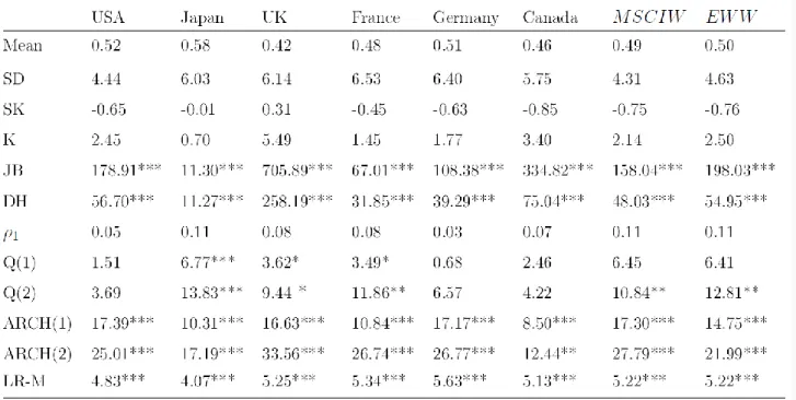
Table 1 reports results from diagnostic tests on our data. As is common with equity returns, there is strong evidence of nonnormality. The autocorrelation coefficients and, to a lesser extent, the Ljung-Box Q statistics indicate the presence of significant autocorrelations, pointing to some short-term predictability of returns even at the monthly frequency. Furthermore, the two ARCH tests reveal significant autoregressive conditional heteroskedasticity for all the series; this motivates the adoption of methods that account for the change in volatility. In the last row, we present standardised Likelihood Ratio statistics for the presence of Markov-switching behaviour in the returns (Hansen, 1992, 1996). The statistics tests the hypothesis of linear variance against the alternative of Markov switching. The results strongly reject the null, everywhere. We therefore proceed and maintain the assumption of heteroskedastic, regime-switching volatility, in keeping with most of the literature (see also Hamilton and Susmel, 1994).

Table 1 - Diagnostic tests for stock returns

Mean is the sample average, SD the standard deviation, SK the skewness coefficient, K the kurtosis coefficient; JB and DH refer to the tests of normality by Jarque and Bera (1987) and Doornik and Hansen (1994), respectively; ρ1 is the

first-order autocorrelation coefficient; Q(k) is the Ljung and Box (1978) statistic for no residual autocorrelation up to lag

k; ARCH(k) is the test for ARCH effects at k-order lags (Engle, 1982); LR − M is the standardized likelihood ratio statistics

for the Markov-switching parameter based on Hansen (1992, 1996). *, **, *** indicate significance at the 10%, 5% and 1% level, respectively.

4.1 Identified common shocks

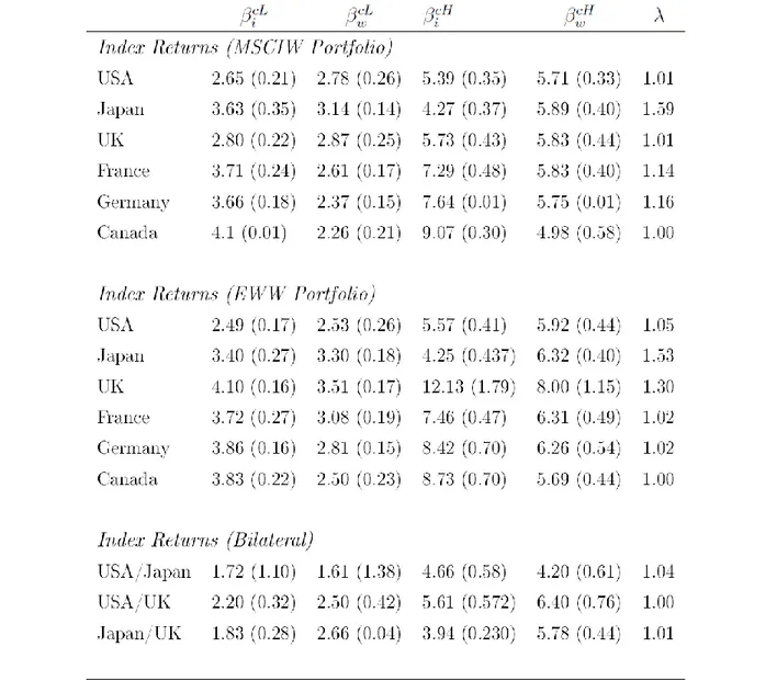
Table 2 reports estimates of some model parameters for common structural shocks (measured in standard deviations). For each country, we report the coefficients that quantify the impact of shocks common to a world portfolio (the value-weighted MSCIW or the equally-weighted index EWW) and to the country index at hand. For completeness, in the bottom panel of the table, we also report estimates of some bilateral

models; for brevity, we limit ourselves to the three largest markets15_{. Estimated parameters refer to the}

low-volatility state (𝛽𝑗𝑐𝐿, 𝛽𝑤𝑐𝐿) and to the high-volatility regime (𝛽𝑗𝑐𝐻, 𝛽𝑤𝑐𝐻).

We observe several interesting patterns. First, as expected, in each country the responses of returns to high-volatility common shocks are markedly larger than those to low-volatility disturbances. In addition, the estimated values of high-volatility impact coefficients tend to vary more widely across markets. Of course, only the statistical analysis of their ratio can tell whether and how impact coefficients vary across volatility regimes. In the case of simple interdependence (only the size of shocks increases), the ratio would not change significantly across regimes, whereas with a strengthened transmission of shocks across countries, i.e., under contagion, the ratio would go up.

Second, estimated impact coefficients for individual countries are very similar no matter whether one employs the MSCIW or the EWW basket as the reference portfolio. This means that our identification scheme captures the systematic components of shocks to volatility in a fashion that is remarkably consistent across portfolios and markets.

Third, during tranquil times the impact of shocks to returns on the US and UK indices, the deepest markets, tend to be smaller than those on most other countries. Index returns for Germany, Canada and France are at the opposite end of the shock distribution. Under high-volatility regimes, those differences disappear.

Fourth, and as expected, in bilateral specifications the size of impact coefficients is on average significantly lower, particularly during tranquil times. This occurs likely because the returns on world market portfolios have a larger exposure to systematic risks.

15 _{In relation to systematic risks, we expect the exposures of returns in the bilateral specifications to have a downward}

Table 2 - Estimates of impact coefficients for common shocks

Estimates of model parameters (expressed in terms of standard deviations) for common structural shocks. For each country, we report the estimated impact of shocks common to a world portfolio (either the value-weighted MSCIW or the equally-weighted index EWW) and to the country index at hand. The bottom panel of the table reports estimates from bilateral models. Parameters refer to the low-volatility state (𝛽𝑗𝑐𝐿, 𝛽𝑤𝑐𝐿) and to the high-volatility regime

(𝛽𝑗𝑐𝐻, 𝛽𝑤𝑐𝐻). Standard errors are reported in parentheses.

To determine whether impact coefficients remain proportional across volatility regimes, let us define by 𝜆 = |𝛽𝑗

𝑐𝐻_𝛽 𝑤 𝑐𝐿

𝛽_𝑗𝑐𝐿𝛽_𝑤𝑐𝐻| the absolute value of the ratio of the impact coefficients in the high volatility regime to the

ratio of the impact coefficients in the low volatility regime. The last column of Table 2 reports its values as implied by our estimates: in most cases, the ratio is very close to one, pointing to the changing size of common shocks as the main reason for closer comovements. However, there are a few cases in which 𝜆 rises further above one. To check whether the ratios of estimated impact coefficients are significantly above one, we follow Gravelle et al. (2006) and construct a simple likelihood ratio test as follows:

𝐻

0

:

𝛽1𝑐𝐻 𝛽2𝑐𝐻

=

𝛽1𝑐𝐿 𝛽2𝑐𝐿 against

𝐻

1

:

𝛽1𝑐𝐻 𝛽2𝑐𝐻

≠

𝛽1𝑐𝐿 𝛽2𝑐𝐿

The implied null hypothesis is that there is no change in the ratio during periods of heightened market volatility and comovement, i.e., there is no contagion. This follows closely definition n. 5 in the well-known taxonomy by Pericoli and Sbracia (2003): (shift-)contagion occurs when the transmission channel intensifies or, more generally, changes after a shock in one market. Our test statistic has a 𝜒2(1) distribution under the null hypothesis. Table 3 contains the test’s results. The statistic is very small in all cases, rising somewhat in the specifications including Japan. The associated p-value confirms that we cannot reject the null hypothesis of no contagion for all the indices pairs. This strong result is consistent with the strand of evidence started by Forbes and Rigobon (2002). This evidence supports the notion that the closer comovement we observe in correspondence of the most recent financial crises is essentially the result of more sizeable common shocks hitting the markets, rather than the effect of increased structural interdependence.

Table 3 - LR test

The implied null hypothesis is that there is no change in the ratio during periods of heightened market volatility, i.e., there is no contagion. The test statistic has a 𝜒2(1) distribution under the null hypothesis (p-values are reported in parentheses).

To gain further insight, in Figures 2-4 we plot the filtered probabilities of high-volatility regimes for common shocks. As before, small black marks on the x-axis denote periods of below-1% GDP growth in the G7 countries, while the shaded areas indicate NBER-dated recessions in the US. The model for the US shows

the highest occurrence of high-volatility periods, with Canada the lowest one, but overall similarities in the displayed patterns are striking. Post mid-1990s, all countries exhibit two major intervals of persistent high volatility of systematic shocks: 1997-2003 and 2008-2013. These periods seem the culmination of financial cycles (Schularick and Taylor, 2012; Miranda-Agrippino and Rey, 2015; Juselius et al., 2016). The average filtered probability as well as the duration of the high-volatility regime (not shown but available on request) are significantly higher after 1996. The charts also show that for all index pairs the timing of prolonged high-volatility spells coincides with that of GDP slowdowns. In particular, the start of US recessions always coincide with a switch to a persistent high-volatility regime. US recessions always precede downturns elsewhere. These findings are in line with those in Corradi et al. (2013) and Kim and Nelson (2014) and are particularly valuable, as here we model the interdependence amongst returns by drawing no information from business-cycle variables. Our estimates of common shocks confirm that the probability of switching from low to high volatility and comovement is dependent on underlying business-cycle conditions, with the latter nicely summarized by NBER-dated peaks and troughs. Therefore, shifts in volatility regimes are likely to occur because of widespread revisions to expectations about underlying macroeconomic fundamentals. Assets’ long-run values are functions of macroeconomic risk factors, which are shared across countries, and of country-specific factors. Increased comovement amongst indices occurs when investors optimally rebalance their portfolio’s exposures to the shared macroeconomic risk factors in other countries’ markets. Our evidence also suggests the presence of cyclical variation in the co-movement across equity indices.

For the US and Japan, our estimates identify several instances in which very synchronous switches to high-volatility regimes took place. For instance: around 1970, 1975, the sharp recessions in the early 1980s, 1987, around 1990, the run-up to the exuberance and subsequent fall of the stock market in 2000, as well as the Great Financial Crisis started in 2007. For all countries, our estimates also signal August 2015 as a switch to high volatility. Strikingly similar too across all index pairs are the intervals of persistent low volatility: indeed, early-to-mid 1990s, 2003-2007 and 2013-2014 stand out as periods of compressed market variability. Other interesting features emerge from individual countries’ filtered probabilities. For instance, volatility states for French and German returns (see Figure 3) look remarkably synchronous, whereas the UK market follows patterns closer to those experienced by the US. Finally, bilateral models in Figure 4, despite being based on more indirect information than (world) market models are, portrait regime switches that are consistent with all other cases. The Japan-UK model in particular points to a relative prevalence of high-volatility states.

FIGURE 2 HERE

Figure 2. Timing of high volatility regimes for common shocks to country index returns against the MSCI World Index

The charts show the filtered probabilities of high volatility regimes for common shocks for the USA, Japan and the UK. For each country, we report the probability associated with shocks common to the world portfolio and to the country index at hand. Lower black marks denote periods during which quarterly GDP growth rate, compared with the same quarter of the previous year and seasonally adjusted, was below 1%; shaded bars indicate NBER-dated recessions of the US economy.

FIGURE 3 HERE

The charts show the filtered probabilities of high volatility regimes for common shocks for France, Germany and Canada. For each country, we report the probability associated with shocks common to the world portfolio and to the country index at hand. Lower black marks denote periods during which quarterly GDP growth rate, compared with the same quarter of the previous year and seasonally adjusted, was below 1%; shaded bars indicate NBER-dated recessions of the US economy.

FIGURE 4 HERE

Figure 4. Timing of high volatility regimes for common shocks to country-pair index returns

The charts show the filtered probabilities of high volatility regimes for common shocks for USA/Japan, Usa/UK, Japan/UK models. Lower black marks denote periods during which quarterly GDP growth rate, compared with the same quarter of the previous year and seasonally adjusted, was below 1%; shaded bars indicate NBER-dated recessions of the US economy.

4.2 Volatility/correlation shifts and business conditions

Given their rich temporal variation, our filtered probabilities provide a valuable opportunity to measure the degree to which regime shifts in volatility and correlation derive from changes in economic activity, market conditions and their uncertainty. In this subsection, we investigate the lead-lag association between the probability of high-volatility states and revisions in the expectations of the business cycle. We perform two complementary exercises for the US. First, we compute monthly correlations of filtered probabilities and a battery of state variables that capture the evolution of expectations about macroeconomic conditions. Second, we run alternative unrestricted bivariate Vector Autoregressions (VAR) of the filtered probabilities and a business cycle indicator. This is in order to gauge the lead-lag relations among the variables.

We chose the following leading indicators of business and financial conditions: the log of the ISM manufacturing PMI (PMI), the 4-week Treasury bill rate (TBILL), the yield spread between ten-year and one-year Treasury bonds (TERM), the yield spread between Moody’s seasoned Baa and Aaa corporate bonds (DEF), the log change in the cyclically-adjusted price/earnings yield by R. Shiller (CAPE) and, in turn, one of three well-known measures of uncertainty. The latter are: the VXO stock market volatility index constructed by the Chicago Board of Options Exchange from the prices of options contracts written on the S&P 100 Index (VXO, monthly average of daily data since 1986), the Financial Uncertainty index (FUNC) and the Macroeconomic Uncertainty index (MUNC), both introduced by Jurado et al. (2015).

Table 4 shows contemporaneous as well as 1- to 3-month lagged and forward correlations. We find that our estimated filtered probabilities correlate more strongly with the indicators of financial uncertainty FUNC and stock market volatility VXO. In particular, the correlation with FUNC, a composite measure of financial uncertainty that aggregates 147 financial time series16_{, is positive and almost always the highest,}

with values ranging from 0.53 to 0.66. Stock market volatility clearly accounts for much of this correlation, as the figures for VXO show. However, both the PMI, which is a leading indicator for the level of economic activity in the manufacturing sector, and MUNC, a composite aggregator of 132 macroeconomic time

16 _{They include valuation ratios such as the dividend-price ratio and earnings-price ratio, growth rates of aggregate}

dividends and prices, default and term spreads, yields on corporate bonds of different ratings grades, yields on Treasuries and yield spreads, and a broad cross-section of industry, size, book-market, and momentum portfolio equity returns (see Jurado et al., 2015).

series17_{, display quite high (and very significant) correlations with our probabilities. In contrast, the short}

interest rate and the long-short spread, commonly used as predictors for economic downturns, have much looser associations. The DEF spread appears to be informationally more relevant, perhaps because of its proven ability to track relative financial distress.

Table 4 - USA, correlations between filtered probabilities of high-volatility regime and selected macroeconomic variables

Contemporaneous, lagged and forward correlations with estimated filtered probabilities of high-volatility state. The variables are: the log of the ISM manufacturing PMI (PMI), the 4-week Treasury bill rate (TBILL), the yield spread between ten-year and one-year Treasury bonds (TERM), the yield spread between Moody’s seasoned Baa and Aaa corporate bonds (DEF), the log change in the cyclically-adjusted price/earnings yield by R. Shiller (CAPE) and, in turn, one of three common measures of: the VXO stock market volatility index constructed by the Chicago Board of Options Exchange from the prices of options contracts written on the S&P 100 Index (VXO, monthly average of daily data since 1986), the Financial Uncertainty index (FUNC) and the Macroeconomic Uncertainty index (MUNC) by Jurado et al. (2015). Values above 0.40 in bold.

Next, we insert the estimated filtered probabilities, along with a business/financial cycle indicator, in a battery of unrestricted bivariate VARs. In order to infer whether the leading indicator Granger-causes, i.e., is helpful in capturing future developments in probabilities, we run Wald tests on the significance of estimated VAR coefficients. The logic of such exercise is straightforward. If markets process information efficiently, and if the probabilities are an unbiased measures of variation in macroeconomic/financial conditions, their dynamics might somehow be predicted by lagged indicators of business fluctuations. If instead probabilities also contain coincident or forward-looking information about macroeconomic risk, their

17 _{This includes broad categories of macroeconomic time series: real output and income, employment and hours, real}

retail, manufacturing and trade sales, consumer spending, housing starts, inventories and inventory sales ratios, orders and unfilled orders, compensation and labor costs, capacity utilization measures, price indexes, bond and stock market indexes, and foreign exchange measures.

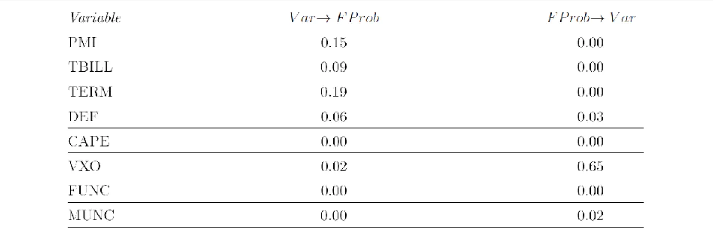
current value might help forecast future business conditions. The VARs lag order is chosen according to conventional information criteria.18,19

Table 5 lists the p-values of Granger-causality tests: a high value points to one variable having low forecasting power for the other. On a comparative basis, our estimated filtered probabilities of the high-volatility regime predict future developments in all indicators except VXO. On the contrary, the forecasting ability of PMI, TBILL and TERM for the probabilities seems very limited. CAPE, VXO, FUNC and MUNC instead all display good predictive content. Therefore, our estimated probabilities contain forward-looking information about developments in macroeconomic conditions, as embodied in commonly used leading indicators such as PMI or TERM, but are not forecast by the latter. This is clear evidence that filtered probabilities, as estimated via our parsimonious approach based only on stock returns, can be used along with state variables to predict future macroeconomic and financial developments. We can also conclude that the observed shifts in the volatility regime are consistent with revisions of market expectations about cyclical and financial conditions. At the aggregate level and in the long run, the dynamics of asset prices should be tied to real variables such as productivity, profitability and demographic factors. Therefore, positive shocks to funding conditions should only drive the transitory components of asset prices. However, over recent cycles the financial sector’s balance sheet has appeared to be particularly vulnerable to fluctuations in risk aversion and asset market expectations, which in turn likely affect business-cycle developments.

18 _{We checked for the robustness of our estimates with respect to the potential bias represented by the use of a}

continuous variable that assumes values in the standard unit interval (0, 1). We applied a variant of the beta

regression model of Ferrari and Cribari-Neto (2004) that allows for nonlinearities and variable dispersion, as proposed by Simas, Barreto-Souza, and Rocha (2010). In this model, the parameter accounting for the precision of the data is assumed to vary across observations, leading to the variable dispersion beta regression model. The results we obtained were not qualitatively different from those without transformation or adjustments of the variables. We thank an anonymous referee for raising this point.

19 _{As standard in many applications (see Hamilton, 1994, and Lutkepohl, 2005, for instance), Granger-causality analysis}

in a bivariate context permits to assess whether one variable contains useful information for improving the

predictions of another variable. It does not describe the full set of interactions between the variables. In cases similar to ours, in which a full-fledged structural model is not at hand, defining and identifying a full VAR system would be impossible. While there would always be some omitted variables, our filtered probabilities are generated variables and their use in overparameterised specifications should be avoided. The solution conventionally adopted in VAR-based Granger-causality tests is to assume that all relevant information is efficiently summarized in the past and current values of the process under study. We therefore follow standard practice by running unrestricted bivariate Vector Autoregressions of our filtered probabilities of high volatility regimes for common shocks along with a business cycle indicator, in order to gauge only the lead-lag relations between the two variables.

Table 5 - USA, VAR Granger-causality tests on filtered probabilities of high-volatility regime and selected macroeconomic variables

P-values of significant (at least 10% confidence level) χ2-statistic of Wald tests on estimated coefficients of unrestricted bivariate VARs of estimated filtered probabilities of high-volatility state (FProb) and a macroeconomic indicator. HAC standard errors were computed (Andrews, 1991). The state variables are: the log of the ISM manufacturing PMI (PMI), the 4-week Treasury bill rate (TBILL), the yield spread between ten-year and one-year Treasury bonds (TERM), the yield spread between Moody’s seasoned Baa and Aaa corporate bonds (DEF), the log change in the cyclically-adjusted price/earnings yield by R. Shiller (CAPE) and one of three common measures of: the VXO stock market volatility index constructed by the Chicago Board of Options Exchange from the prices of options contracts written on the S&P 100 Index (VXO, monthly average of daily data since 1986), the Financial Uncertainty index (FUNC) and the Macroeconomic Uncertainty index (MUNC) by Jurado et al. (2015).

5 Conclusions and implications

We enrich the evidence regarding international equity return comovements by establishing the following stylized facts. First, our estimated probabilities of a high-volatility, high-correlation regime are strongly associated with measures of macroeconomic uncertainty. Persistent high-volatility spells mostly coincide with macroeconomic slowdowns, which in turn trigger increases in cross-market correlations. This confirms that shifts in the regime of volatility and comovement of equity indices are likely the result of revisions in the subjective probability distribution of macroeconomic risks and hence of expectations about underlying business conditions. Second, the exposure of returns to common shocks is significantly larger during times of high volatility. Third, this increase in the observed responses of international stock returns to common shocks is largely attributable to the occurrence of bigger shocks (heteroskedasticity of fundamentals) rather than to breaks in the transmission mechanism or contagion between markets. In addition, as the structural linkages across markets appear overall stable, international diversification is still effective in mitigating risk during episodes of market turbulence. Fourth, since the late 1990s correlations between international stock indices appear to have stepped up. Our estimates confirm that returns have since then entered more often a regime of high volatility likely because of more sizeable and persistent macroeconomic disturbances. Of course, the question of the origins and nature of those larger perturbations remains to be answered, as well as that of the role of uncertainty (Bansal et al., 2014; Baker et al., 2016).

These results suggest that while variances and covariances across markets do shift over time, the spillover effects are essentially a function of the magnitude of cross-country shocks rather than of breaks to

the transmission mechanism. In other words, variances, covariances and correlations are both time and state varying and mainly reflect the size of systematic shocks.

These results have implications along several, important dimensions. Policy makers aim at minimizing financial stability risks and their effects on real activity. Financial investors care about the impact that changes in correlations exert on the pricing and hedging of portfolio risks. Equity returns are correlated with business cycles: at the trough of downturns, expected returns and risk premia are high (equity prices are low), whereas they are low (prices are high) close to boom peaks. The market prices of risk vary over time, and as a result, they induce time variation in both the volatility and correlation of returns. When market volatility and correlation are high, increased risk will be compounded by a decline in diversification potential. In the medium term and at frequencies that are consistent with the standard rebalancing of portfolio choices, the difference between normal and increased structural interdependence surely matters to investors. Moreover, we gather evidence of an increasing occurrence of large macroeconomic disturbances as determinants of heightened volatility and correlation in asset returns. This confirms that there is not only an intuitive causal relationship from economic activity to funding conditions and on to asset price changes and valuations, but also a positive feedback response of asset prices on to monetary conditions, and so forth, along a mutually reinforcing, and potentially destabilizing, loop (Schularick and Taylor, 2012, for instance). This complex interdependence has likely become stronger with the rise in importance of some relatively new channels of liquidity creation. As a result, macroeconomic policies should take financial developments more systematically into account. The optimal asset weights in internationally diversified portfolios change with expected returns, volatilities, and correlations of the assets. The resulting portfolio rebalancing may affect the dynamics of returns on all assets, particularly across international financial markets that are increasingly integrated at a global level. One interesting extension would be to investigate the degree of interdependence amongst returns on bond, stock and currency markets, particularly around the Great Financial Crisis.

6 References

Ang, A., and J. Chen, 2002. Asymmetric correlations of equity portfolios. Journal of Financial Economics, 63, 443-494.

Ang, A. and G. Bekaert, 2002. International Asset Allocation with Regime Shifts. Review of Financial Studies, 15 (4), 1137-1187.

Ang, A., and A. Timmermann, 2012. Regime Changes and Financial Markets. Annual Review of Financial Economics, 4:313-337.

Baele, L., G. Bekaert, and K. Inghelbrecht, 2010. The Determinants of Stock and Bond Return Comovements. Review of Financial Studies, 23:6, 2374-2428.

Baele, L. and K. Inghelbrecht, 2009. Time-varying integration and international diversification strategies. Journal of Empirical Finance, 16 (3), 368-387.

Baig T. and I. Goldfajn, 1999. Financial Market Contagion in the Asian Crisis. IMF Staff Papers, Palgrave Macmillan, vol. 46(2).

Baker, Steve, N. Bloom, and S. Davis, 2016. Measuring Economic Policy Uncertainty. Quarterly Journal of Economics, 131 (4): 1593-1636.

Bansal, R., D. Kiku, I. Shaliastovich and A. Yaron, 2014. Volatility, the Macroeconomy and Asset Prices. Journal of Finance, 69 (6), 2471-2511.

Bekaert, G. and C. R. Harvey, 1995. Time-varying world market integration. Journal of Finance, 50, 403- 444.

Bekaert, G., M. Ehrmann, M. Fratzscher, and A. J. Mehl, 2014. Global Crises and Equity Market Contagion. Journal of Finance, 69:6, 2597-2649.

Bekaert, G. and C. R. Harvey, 1997. Emerging equity market volatility, Journal of Financial Economics, 43, 29--77.

Bekaert, G., C. R. Harvey and R. Lumsdaine, 2002. Dating the integration of world equity markets. Journal of Financial Economics, 65 (2), 203-248.

Bekaert, G., C. R. Harvey and C. Lundblad, 2005. Does financial liberalization spur economic growth. Journal of Financial Economics, 77, 3-55.

Bekaert, G., C. R. Harvey and C. Lundblad, 2006. Growth volatility and financial liberalization. Journal of International Money and Finance, 25, 370-403.

Bekaert, G., C. R. Harvey, C. Lundblad and S. Siegel, 2007. Global growth opportunities and market integration. Journal of Finance, 62 (3), 1081-1137.

Bekaert, G., C. R. Harvey, C. Lundblad and S. Siegel, 2011. What segments equity markets?. Review of Financial Studies, 24:12, 3847-3890.

Bekaert, G., R. Hodrick and X. Zhang, 2009. International stock return comovements. Journal of Finance, 64, 2591-2626.

Brière, M., A. Chapelle, and A. Szafarz (2012). No contagion, only globalization and flight to quality. Journal of International Money and Finance, 31(6), 1729-1744.

Bruno, V., and H.S. Shin (2015). Capital flows and the risk-taking channel of monetary policy. Journal of Monetary Economics, 71, 119-132.

Candelon, B., Hecq, A., Verschoor, W.F.C., 2005. Measuring common cyclical features during financial turmoil: Evidence of interdependence not contagion. Journal of International Money and Finance, 24, 1317-1334.

Caporale, G.M., Cipollini, A., Spagnolo, N., 2005. Testing for contagion: A conditional correlation analysis. Journal of Empirical Finance 12, 476-489.

Corradi, V., W. Distaso, A. Mele, 2013. Macroeconomic determinants of stock volatility and volatility premiums. Journal of Monetary Economics, 60, 203--220.

Corsetti, G., Pericoli, M., Sbracia, M., 2005. Some contagion, some interdependence: More pitfalls in tests of financial contagion. Journal of International Money and Finance 24, 1177-1199.

David, A. and P. Veronesi, 2013. What Ties Return Volatilities to Price Valuations and Fundamentals? Journal of Political Economy, 121:4, 682-746.

Doornik, J.A., and H. Hansen, 1994. A practical test for univariate and multivariate normality. Discussion Paper, Nuffield College.

Dungey, M., Fry, R., Gonzalez-Hermosillo, B., Martin, V.L., 2006. International contagion effects from the Russian crisis and the LTCM near-collapse. Journal of Financial Stability, 2, 1-27.

Dungey, M., Martin V.L., 2007. Unravelling financial market linkages during crises. Journal of Applied Econometrics, 22, 89-119.

Engle, R.F., 1982. Autoregressive conditional heteroscedasticity, with estimates of the variance of United Kingdom inflation. Econometrica, 50, 987-1007.

Fama, E., and K. French, 1998. Value versus growth: The international evidence. Journal of Finance, 53, 1975-1999.

Ferrari, S., and F. Cribari-Neto, 2004. Beta regression for modelling rates and proportions. Journal of Applied Statistics, 31 (7), 799-815.

Ferson, W.E., and C.R. Harvey, 1993. The risk and predictability of international equity returns. Review of Financial Studies, 6, 527-566.

Flavin, T. J., E. Panopoulou and D. Unalmis, 2008. On the stability of domestic financial market linkages in the presence of time-varying volatility. Emerging Markets Review, 9(4), 280-301.

Flavin, T. J. and E. Panopoulou, 2009. On the robustness of international portfolio diversification benefits to regime-switching volatility. Journal of International Financial Markets, Institutions and Money, 19(1), 140-156.

Flavin T. and E. Panopoulou, 2010. Detecting Shift And Pure Contagion In East Asian Equity Markets: A Unified Approach. Pacific Economic Review, 15(3), 401-421.

Forbes, K.J., Rigobon, R., 2002. No contagion, only interdependence: measuring stock market comovements. Journal of Finance, 57, 2223--2261.

Gravelle, T., M. Kirchian and J.C. Morley, 2006. Detecting Shift-Contagion in Currency and Bond Markets. Journal of International Economics, 68, pp. 409-423.

Hamilton, J.D., and G. Lin, 1996. Stock market volatility and the business cycle. Journal of Applied Econometrics, 11 (5), 573--593.

Hamilton, J.D., and R. Susmel, 1994. Autoregressive conditional heteroskedasticity and changes in regime. Journal of Econometrics, 64, 307-333.

Heston, S. L. and K. G. Rouwenhorst, 1994. Does industrial structure explain the benefits of international diversification? Journal of Financial Economics, 36, 3-27.

Imbs, J., 2004. Trade, finance, specialization and synchronization. Review of Economics and Statistics, 86 (3), 723-734.

Jappelli, T. and M. Pagano, 2008. Financial market integration under EMU. CEPR Discussion Paper No. 7091.

Jarque, C.M., and A.K. Bera, 1987. A test for normality of observations and regression residuals. International Statistical Review, 55, 163-172.

Jurado, K., S.C. Ludvigson, S. Ng, 2015. Measuring Uncertainty. American Economic Review, 105(3), 1177-1216.

Juselius, M. C. Borio, P. Disyatat and M. Drehmann, 2016. Monetary policy, the financial cycle and ultra-low interest rates. BIS Working Paper 569.