About the development of visual search algorithms and their hardware implementations

(1)

Dottorato in Informatica e Ingegneria dell’Informazione Curriculum Informatica

Coordinatore: Prof. Alfredo De Santis

XV Nuovo Ciclo

About the Development of Visual Search Algorithms and

their Hardware Implementations

Relatori:

Ch.mo Prof. Giancarlo Raiconi Ph.D. Mario Vigliar

Candidato: Luca Puglia Matr. 8888100007

(2)

(3)

“...Inside my heart is breaking My make-up may be flaking But my smile still stays on...” — The Show Must Go On, Queen

(4)

(5)

Introduction

The main goal of my work is to exploit the benefits of a hardware imple-mentation of a 3D visual search pipeline. The term visual search refers to the task of searching objects in the environment starting from the real world representation. Object recognition today is mainly based on scene descriptors, an unique description for special spots in the data structure. This task has been implemented traditionally for years using just plain images: an image descriptor is a feature vector used to describe a position in the images. Matching descriptors present in different viewing of the same scene should allows the same spot to be found from different angles, therefore a good descriptor should be robust with respect to changes in: scene luminosity, camera affine transformations (rotation, scale and trans-lation), camera noise and object affine transformations. Clearly, by using 2D images it is not possible to be robust with respect to the change in the projective space, e.g. if the object is rotated with respect to the up camera axes its 2D projection will dramatically change. For this reason, alongside 2D descriptors, many techniques have been proposed to solve the projective transformation problem using 3D descriptors that allow to map the shape of the objects and consequently the surface real appearance. This category of descriptors relies on 3D Point Cloud and Disparity Map to build a reliable feature vector which is invariant to the projective transformation. More

(10)

sophisticated techniques are needed to obtain the 3D representation of the scene and, if necessary, the texture of the 3D model and obviously these techniques are also more computationally intensive than the simple image capture. The field of 3D model acquisition is very broad, it is possible to distinguish between two main categories: active and passive methods. In the active methods category we can find special devices able to obtain 3D information projecting special light and. Generally an infrared projector is coupled with a camera: while the infrared light projects a well known and fixed pattern, the camera will receive the information of the patterns reflection on a certain surface and the distortion in the pattern will give the precise depth of every point in the scene. These kind of sensors are of course expensive and not very efficient from the power consumption point of view, since a lot of power is wasted projecting light and the use of lasers also imposes eye safety rules on frame rate and transmissed power. Another way to obtain 3D models is to use passive stereo vision techniques, where two (or more) cameras are required which only acquire the scene appearance.

Using the two (or more) images as input for a stereo matching algorithm it is possible to reconstruct the 3D world. Since more computational resources will be needed for this task, hardware acceleration can give an impressive performance boost over pure software approach.

In this work I will explore the principal steps of a visual search pipeline composed by a 3D vision and a 3D description system. Both systems will take advantage of a parallelized architecture prototyped in RTL and implemented on an FPGA platform. This is a huge research field and in this work I will try to explain the reason for all the choices I made for my implementation, e.g. chosen algorithms, applied heuristics to accelerate the performance and selected device. In the first chapter we explain the Visual Search issues, showing the main components required by a Visual Search pipeline. Then I show the implemented architecture for a stereo vision system based on a Bio-informatics inspired approach, where the final system can process up to 30fps at 1024 × 768 pixels. After that a clever method for boosting the performance of 3D descriptor is presented and as last chapter the final architecture for the SHOT descriptor on FPGA will

(11)

CONTENTS 11

be presented. A more complete description of the work can be found in [1,2,3,4,5,6]

(12)

(13)

Chapter

1

Visual Search

Visual Search is a complex task and over the years many approaches have been proposed to solve it. Since the real world can be modelled with different kinds of data, visual search methods may differ a lot with respect to the chosen technique. Generally speaking, a representation of the real world can be acquired in multiple ways. Two kinds of sensors are used in this field: camera sensors and range sensors. Both sensors have advantages over the other. the images produced with a camera are relatively easy to manipulate and visualize but a slanted surface in the scene will result in major drawback in the visual search algorithm performance (in Fig. 1.1 is shown an instance of the problem). By using a range sensor it is possible to obtain a 3D representation of the world, but unfortunately this representation is less compact than an image but more information about the scene structure is carried by the data (Fig. 1.2); furthermore, changes in the position of the sensors potentially bring projective changes in the object pose, and a change in the object projection onto the image plane will dramatically change the appearance of some object, using a 3D representation no problems arise when the object is rotated since the whole structure is defined.

In order to have better results in the Visual Search pipeline, we decided to 13

(14)

Figure 1.1: Example of visual search problem using images; starting from a template (left) some keypoints are extracted, using a visual search algorithm is possible to match these points in a cluttered scene (right). This kind of approach only works well when the template pose is close to the one present in the scene.

utilize the more robust representation brought by range sensors. This kind of data are more complex to acquire. Usually each device uses its own output format and a conversion phase is required to use those data. These systems can be distinguished in active and passive. The former category uses a light sensor paired with a light emitter, the emitter projects a pattern over the scene, while the sensor registers changes in the known pattern; By using this strategy it is possible to measure the distances of the scene positions. Some drawbacks occur when using these sensors in outdoor enviroment and direct sunlight: in fact, sun rays can interfere with the light emitter pattern. Some of these systems are available off-the-shelf (e.g. KinectTM, Asus Xtion Pro Live, ...). The latter category, instead, is based on just camera sensors. By using images, in fact, it is possible to obtain information about the object position, the system generally results more power efficient than an active approach since no light emitters are used, but of course more computational power is required because a complex algorithm must run.

For this work I created range data starting from a camera pair (so the passive approach was chosen). Starting from a stereoscopic system it is

(15)

1.1. ACTIVE RANGE SENSORS 15

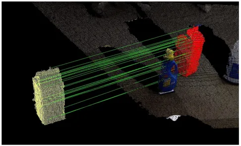
Figure 1.2: Example of 3D visual search, the template in yellow (on the left) is matched against the 3D representation of the scene (on the right).

possible to obtain a 3D representation of the scene, but, as mentioned previously, more computational power is required.

1.1 Active range sensors

In the past few years there has been a growing interest in processing 3D data. Computer vision tasks such as 3D keypoint detection and description, surface matching and segmentation, 3D object recognition and categorization have become of major relevance. The relevance of such applications has been fostered by the availability, in the consumer market, of new low-cost Active range sensors (also called RGB-D cameras), which can simultaneously capture RGB and range images at a high frame rate. Such devices are either based on structured light (e.g. Microsoft Kinect, Asus Xtion) or Time-of-Flight (TOF) technology (e.g., Kinect II) (Fig. 1.3), and belong to

(16)

Figure 1.3: Example of off-the-shelf RGB-D sensors.

the class of active acquisition methods.

Independently from the specific technology being used, each sensor acquires 3D data in the form of range images, a type of 3D representation that stores depth measurements obtained from a specific point in 3D space (i.e., sensor viewpoint) — for this reason, it is sometimes referred to as 2.5D data. Such representation is organized, in the sense that each depth value is logically stored in a 2D array, so that spatially correlated points can be accessed by looking at nearby positions on such grid. Conversely, data are unorganized when 3D representation is simply stored in 3D coordinates in an unordered list. These kinds of representation (unorganized and organized) are called point clouds.

1.2 Passive range sensors

Stereo Matching is the problem to solve to obtain a 3D representation of the world. In order to triangulate every point in the scene a special pair of sensors is required. This problem usually requires two cameras as input sources. It can be defined as the process of finding couples of pixels in the two images representing the same points in the real world. It is possible to distinguish two categories of problems, namely: sparse stereo matching and dense stereo matching. The first category is generally easier and faster to solve since only some specific (key)points are matched between the images

(17)

1.2. PASSIVE RANGE SENSORS 17

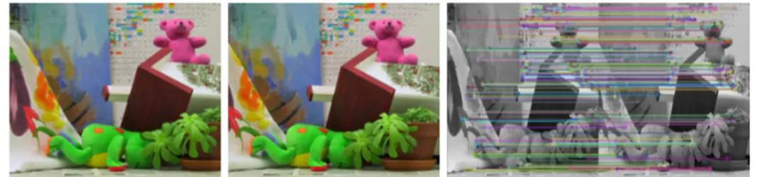
Figure 1.4: Sparse stereo matching input (first two images) and output (last image). The horizontal lines represent the few matched point on both

images.

(Fig. 1.4). The second category can be thought as a generalization of the first one: instead of finding just some matches in the two images, a match is find for every point (pixel) (Fig. 1.5); the final result of this process is called a disparity map.

Figure 1.5: Dense stereo matching problem input (first two images) and output (last two images).

Since [7] all the efforts in the Stereo Vision community have been focused on finding the best algorithm to match correct pixel pairs. Many of these algorithms are discussed in [8], where a taxonomy is defined that distin-guishes between global and local methods. According to [8] Stereo Vision algorithms are composed of five different phases:

• Pre-processing;

(18)

• Cost aggregation; • Disparity computation; • Disparity refinement.

The search for the best method has caused an explosion of creativity regard-ing the matchregard-ing technique. Disparity map quality, system performance, frame rate, image resolution, power consumption and platform cost are just few of the objectives that can be achieved by a stereo vision system. Obviously, many of these targets are in contrast, e.g. it is not possible to have good disparity map quality with high performance on a cheap platform, therefore a trade-off has to be reached. The complexity of the algorithm impacts on the disparity map quality, in fact, it is tightly coupled to the number of comparisons to be performed: for every pixel in the first (reference) image a matching pixel must be found in the second (target)

image.

1.2.1 Pre-processing

This is a common phase for every image processing algorithm, in the stereo-vision context is used to remove image distortion and noise. The following methods are encompassed by the pre-processing:

• Laplacian of Gaussian (LoG) filtering [9]; • Histogram equalization;

• Neighborhood average value subtraction [10]; • Bilateral filter [11].

(19)

1.2.2 Matching Cost

Since a comparison between pixels is required a matching cost function must be defined, the easiest technique is to subtract pixel channel values: let I_L be the reference image (sensor on the left), IR be the target image (sensor

on the right), we define:

• Absolute intensity difference (AD): |IL(x1, y1) − IR(x2, y2)|

• Squared intensity difference (SD): (IL(x1, y1) − IR(x2, y2))2

where I(x, y) represents the pixel of position x, y.

1.2.3 Disparity Computation

Once a cost function is defined it is possible to compute the disparity between pixels. The plot in Fig. 1.6 is obtained by comparing pixels on the left image with every single pixels in the homologous right line.

If the cost function is good enough, the function minima will represent the correct match and consequently the disparity. This kind of strategy has been named "winner takes all" (WTA) (see Fig. 1.7). By using this kind of strategy it is hard to obtain good results since the cost function has to be robust enough to accounnt for every possible situation present in the images.

1.2.4 Cost Aggregation

In order to obtain a more robust algorithm it is possible to aggregate the cost functions of more than one pixel:

X

(x,y)∈W

(20)

d

Matching Cost

d

_max

Figure 1.6: Disparity Function.

This function is called SAD (Sum of Absolute intensity Differences) or SSD (Sum of Squared intensity Differences) if the square value is used. In this case a window of pixels W is used to compute the cost of the matching. Fig.

1.8 shows how much the final result is improved.

1.2.5 Disparity Refinement

In order to enhance the final results of Cost Aggregation, a post-processing phase of disparity refinement is applied. Since the relative pixel distances are always integer numbers, the disparity function acts as if the world is discrete, but this is obviously not true for the real world. To improve the final result the disparity function could be interpolated to give a more smooth appearance to the disparity map (Fig. 1.9).

Furthermore, a cost aggregation strategy will decrease the quality of the disparity map around the corners; this happens because the different point of view between the cameras change dramatically the object projections

(21)

reference image ground truth ﬁnal result

Figure 1.7: Winner takes all applied to Absolute intensity Difference.

reference image ground truth ﬁnal result

Figure 1.8: Winner takes all applied to Sum of Absolute intensity Differences.

close to the edges, for this reason running an outlier detector/corrector increases the overall quality (Fig. 1.10).

1.2.6 Main Problems

Using window approaches (SAD, SSD) has some drawbacks. The main problems to address are the following:

• object edges; • repetitive texture; • uniform areas; • small structure.

(22)

d

Matching Cost

d

_max

Figure 1.9: Interpolated Disparity Function.

In Fig. 1.11some instances of these problems are shown.

In square 1 repetitive textures are present caused by multiple books with the same cover; in squares number 2 and 3 flat zones are highlighted; in square number 4 a slanted surface does not allow an easy matching; in 6 and 7 the edges of the objects affect the accuracy, finally in 5 the window is larger than the contained object.

1.2.7 Global Techniques

The methods shown in the previous sections are called local because they utilize only local information to match pixels, however other kinds of local methods use more complicated matching criteria based on correlation [12] and variable size windows [13,14]. In order to obtain better results, a global method could be applied: these methods use whole image chunks during the optimization of the global function.

(23)

Figure 1.10: Outlier detection and correction.

1 2

3

4 5

6 7

Figure 1.11: Windows which are responsible for major drawbacks in the result quality.

image; the functions depend on the parameter δ which represents the relative offset in the image space:

d(x, y) = argmin

δ

(∆(I_L(x, y), I_R(x + δ, y)))

The matching problem is now converted into an optimization problem. By minimizing the function for each pixel (x, y) we obtain a monochrome disparity map in which color channel are substituted by the solution d(x, y). The ∆ function can be defined as explained above using SAD and SSD functions:

(24)

d(x, y) = argmin δ   X (x,y)∈W

∆(I_L(x, y), I_R(x + δ, y))  

This method enhances the quality of the algorithm in plain zones but deteriorate the quality near the object edges.

1.2.8 Accelerating Stereo Vision

Depending on the technique chosen, stereo matching can be a complex and time-consuming task, which makes CPU implementation very expensive (or unfeasible for global methods) in terms of cost of the chip and power consumption, and consequently a very large number of implementations for both GPU and FPGA devices have been developed in recent years. A remarkable GPU implementation can be found in [15] in which an Absolute Difference (AD)-Census algorithm is implemented; this algorithm has been ranked first in the Middlebury benchmark [16]. GPUs are chosen for the native support for parallelism, in fact many cores on a GPU can process multiple pixel pairs at the same time reducing dramatically the processing time. But the shortcoming of this approach is power consumption: generally a desktop GPU consumes many tens of watts making this solution not valid for embedded applications. In recent years many artificial vision applications on mobile robot have been developed, one of the principal tasks to handle in building a fleet of robots is the power management and the cost of the single element, without an affordable and power efficient solution further progress in this field will be constrained. The only way to obtain a stereo vision system with a low power consumption and acceptable quality on a cheap device is to use a dedicated architecture, that can be produced using devices like FPGA and ASIC. Since ASIC requires thousands (if not millions) devices to be produced, in this work I have prototyped an FPGA architecture. For a more accurate comparison between GPU and FPGA limits see [17].

(25)

1.3. DIFFERENCES BETWEEN ACTIVE AND PASSIVE SENSORS 25

1.3 Differences between Active and Passive

sen-sors

The principal difference between active and passive range sensors is the resultant output: generally, an active sensor will output a point cloud, while a passive system will output a disparity map. Luckily both formats are interchangeable, therefore, starting from one is possible to obtain the other (with a modest numeric precision loss in the distances).

Since my visual search pipeline will be composed of a stereo vision system and a 3D description module, a conversion from disparity map to point cloud is requieed. The conversion is straightforward, each pixel becomes a point. The conversion formula is based on the camera parameters and the baseline size between the two cameras.

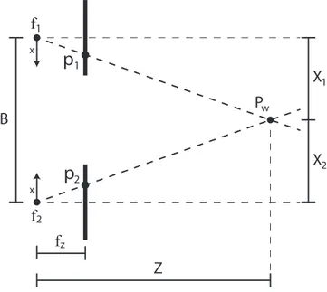
In1.13a classic structure for stereo vision system is shown: the vertical bold lines represent the image planes of the cameras, each camera has a focus f and a focus length f_z. In stereo systems, it is common to have homogeneous sources, thus a set of identical cameras with same f_z is used. A baseline B represents the distance between the two focuses, while the distance from a point in the real word P_w to the baseline is Z. The projection of the point Pw onto the camera sensors is marked respectively by p1 = (x1, y1) and

p2 = (x2, y2). By orienting the reference system of both cameras inward it

is possible to simplify the equation to represent the disparity d of the point Pw as the sum of x coordinate of p points:

d = x1+ x2

This disparity is inversely proportional to the distance and can be used to triangulate the Z of the real world point. By using triangular similarity it is possible to obtain the following equation system:

       X1 Z = x1 fz X2 Z = x2 fz X1+ X2 = B

(26)

Figure 1.12: Disparity to cloud result.

This system can be solved for Z to obtain:

Z = Bfz d

by applying this rule to every disparity in the disparity map a point cloud is built.

(27)

1.4. 3D DESCRIPTORS 27

P

p

1

f

1 2

B

Z

f

z

X

1

X

2 w x x

p

2

Figure 1.13: Scheme of a stereo system as it appears from the top.

1.4 3D Descriptors

The technological progress in the development of range sensors has led us to the ability in delivering high definition range map with an high frame rate. Each process that needs to be applied to this range map stream (e.g. key points extraction and key points description) has to satisfy a precise performance constraint in order to avoid bottlenecks in computation. To execute these algorithms on portable devices the extra constraint of low power usage is imposed.

The principal problem to address during 3D scene reconstruction is to find the correct rotation and translation matrix among many views obtained through passive or active range sensors (also called depth sensors).

(28)

a 3D point (x, y, z) and an optional colour. Aligning point clouds is not easy and it is strictly related to the Simultaneous Localization and Mapping (SLAM) problem, but, once two disparity maps are correctly aligned, the

relative positions of the sensors could be easily computed.

To solve the point cloud alignment problem is possible to use techniques based on the point matches among clouds. To make a correct match, it is necessary to compute a unique and descriptive representation for each point that is invariant to the sensor pose. For this reason, if this representation remains unambiguous among the views, it is said to be the “description” of the point. Specifically speaking, the description (or descriptor) of the point is stored as a multidimensional feature vector. The similarity between two descriptions is easily computed as the distance in the features space of the descriptors.

As keypoint extractions and descriptions are computationally intensive, these tasks are not suitable for embedded applications which require real time performance. Even modern Desktop CPUs struggle trying to compute a large number of descriptors of a 3D point cloud video. A possible solution is to use a GPU to parallelize the processing, but a battery dependent application could never use such a power consuming device, e.g. a drone trying to reconstruct the environment and at the same time to localize itself in the real word will never have the ability to align 3D cloud points obtained using a depth sensor. The only way to obtain a high performance system with a low power consumption and acceptable quality is to use a dedicated architecture that can be produced using devices like FPGA and ASIC. Since ASIC requires thousands (if not millions) devices to be produced, I chose to develop my application using an FPGA.

To avoid problems caused by rigid rotation of the objects, it is essential to define a reference system. The older techniques use the so called Local Reference Axis (LRA) which use the normal of the keypoint as a reference axis, while more recent approaches use a Local Reference Frame (LRF). A LRF is a new coordinate system that is used as a reference to encode the various geometries of the neighborhood. The LRF can be thought of

(29)

as a way to make the descriptors invariant to the sensor pose; this result is obtained by using the LRF as a way to encode the neighborhood of a keypoint.

Several 3D local feature descriptors have been designed to encode the in-formation of a local surface. Among these approaches, many algorithms use histograms to represent different characteristics of the local surface. Specifically, they describe the local surface by accumulating geometric or topological measurements (e.g., point numbers) into histograms according to a specific domain (e.g., point coordinates, geometric attributes). These al-gorithms are categorized into ’spatial distribution histogram’ and ’geometric attribute histogram’ based descriptors. (Fig. 1.14).

1.4.1 Histogram based Descriptors

In this category we can find descriptors that use the point positions to build histograms.

Spin Image (SI) [19, 20] (Fig. 1.14.a) in SI the normal n to keypoint k is used as LRA, for each point q_i in the neighborhood an α and a β parameter are computed (Fig. 1.14.a). The discretization of these two distances is used to build a 2D Histogram, each point is accumulated in the histogram giving the final SI descriptor.

3D Shape Context (3DSC) [21] in 3DSC the normal n to keypoint k is used as the LRA. A spherical grid is superimposed on p, with the north pole of the grid being aligned with the normal n. The grid is then divided into several bins (Fig. 1.14.b). The divisions are logarithmically spaced along the radial dimension and linearly along the other two dimensions. The 3DSC descriptor is computed by counting the weighted number of points laying into each bin.

Unique Shape Context (USC) [22] USC is an extension of 3DSC which is more robust to the rotation and translation changes. The LRF is used instead of the LRA and it is computed starting from the neighborhood instead of the normal n to keypoint k (Fig. 1.14.c).

(30)

(a) (e) ( ) f ( g (h)) ) c ( ) b ( (d) (i) (j)

(31)

Rotational Projection Statistics (RoPS) [23,24] RoPS is based on a novel, unique and repeatable LRF [24]. According to the LRF the points are rotated around the three coordinate axis. For each rotation the pro-jection onto the xy, yz and xz space is performed and for each propro-jection a distribution matrix is generated, which is used to encode five statistics. RoPS descriptor will be built starting from the concatenation of all the statistics (Fig. 1.14.e).

Tri-Spin-Image (TriSI) [25] TriSi builds a LRF in a similar way as it is done in RoPS. The surface is rotated according to the LRF and then a spin image is generated using the x-axes as its LRA. In addition, another two spin images are computed using the y and z-axes as the LRAs of these spin images (Fig. 1.14.d). The TriSI descriptor is formed by concatenating the spin images.

1.4.2 Geometric Attribute Histogram based Descriptors These descriptors represent the local surface by generating histograms according to the geometric attributes (e.g., normals, curvatures) of the points on the surface.

Local Surface Patch (LSP) [26, 27] In LSP, the shape index [28] and the cosine of the angle between the normal of the neighboring points and the keypoint normal are calculated. The LSP descriptor is a 2D histogram, where the shape index value and the cosine of the angle between the normals are discretized in bins (Fig. 1.14.f).

THRIFT [29, 30] In THRIFT, a 1D histogram of the deviation angles between the normal of the keypoint k and normals of the neighboring points is built (Fig. 1.14.g). The density of point samples and the distance from the neighboring point to the keypoint are used to update the bins in a histogram.

Point Feature Histogram (PFH) [31] in PFH, for each pair of points in the neighborhood, a Darboux frame is defined using the normals and point

(32)

coordinates (Fig. 1.14.i). Next, four features are calculated for each point pair using the Darboux frame, the surface normals, and their positions. PFH is generated by accumulating points in particular bins along the four dimensions.

Fast Point Feature Histogram (FPFH) [32] First of all, a simplified point feature histogram (SPFH) is generated for each point by calculating the relationships between a point and its neighbors (Fig. 1.14.h). While in PFH there is the comparison between all the pairs in the neighborhood. FPFH is then built as a weighted sum of all the SPFH built upon every point in the neighborhood.

Signature of Histogram of Orientations (SHOT) [22] First, an LRF is computed for the keypoint k, then the neighboring points are aligned with this new LRF. Next, the support region is divided into several volumes along the radial, azimuth and elevation axes (Fig. 1.14.j). A local histogram is associated to each volume. The histograms are filled according to the angles between the normals to the neighboring points and the normal to the keypoint. The SHOT descriptor is the concatenation of all the local histograms. For further reading on the topic refer to [18].

(33)

Chapter

2

Tools

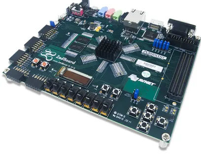
The present work of research has been completed using mainly Altera and Xilinx Tools and its Intellectual Properties (IP). Prototyping a new architecture starting from scratch is not a simple task, for this reason Altera and Xilinx tools come in help to the hardware designer. The developed IPs were produced using Verilog and High Level Synthesis (HLS) by Xilinx languages. The board used to prototype the proposed system is a Zedboard (Fig. 2.1) mounting a Zynq 7000 chip (part number: xc7z020clg484-1). The Zynq 7000 family is very handy when used in prototyping, in fact, the programmable logic is coupled with an ARM dual-core A9. ARM core is crucial when an actual debug on the circuit takes place, in fact, it is easier to feed simulated data to the architecture using a microprocessor. The ARM core is able to run both bare metal applications and Linux kernel, making even easier the architecture debugging. Furthermore, for every IP present in the Xilinx IP catalog a Linux driver is available, speeding up the prototyping time.

(34)

Figure 2.1: Zedboard.

2.1 ModelSim Altera Edition

Producing an IP could be a frustrating process, hours and hours spent simulating the circuits just to notice an error in the signal stimulations. The simulation is a critical task before the actual synthesis. For this purpose a lot of tools are available on the market and one of the best is without any doubt ModelSim Altera Edition (Fig. 2.2).

ModelSim combines simulation performance and capacity with the code coverage and debugging capabilities required to simulate multiple blocks and systems and attain ASIC gate-level sign-off. Comprehensive support of Verilog, SystemVerilog for Design, VHDL, and SystemC provide a solid foundation for single and multi-language design verification environments. ModelSim’s easy to use and unified debug and simulation environment provide today’s FPGA designers both the advanced capabilities that they

(35)

2.1. MODELSIM ALTERA EDITION 35

Figure 2.2: ModelSim Altera Edition.

are growing to need and the environment that makes their work productive. The ModelSim debug environment’s broad set of intuitive capabilities for Verilog, VHDL, and SystemC make it the choice for ASIC and FPGA design. ModelSim eases the process of finding design defects with an intelligently engineered debug environment. The ModelSim debug environment efficiently displays design data for analysis and debug of all languages.

ModelSim allows many debug and analysis capabilities to be employed post-simulation on saved results, as well as during live simulation runs. For example, the coverage viewer analyzes and annotates source code with code coverage results, including FSM state and transition, statement, expression, branch, and toggle coverage.

Signal values can be annotated in the source window and viewed in the waveform viewer, easing debug navigation with hyperlinked navigation between objects and its declaration and between visited files.

(36)

Figure 2.3: Xilinx Vivado.

Race conditions, delta, and event activity can be analyzed in the list and wave windows. User-defined enumeration values can be easily defined for quicker understanding of simulation results. For improved debug productivity, ModelSim also has graphical and textual dataflow capabilities.

2.2 Xilinx Vivado Design Suite

Vivado enables developers to synthesize their designs, perform timing analy-sis, examine RTL diagrams, simulate a design’s reaction to different stimuli, and configure the target device with the programmer. Vivado is a design environment for FPGA products from Xilinx, and is tightly-coupled to the architecture of such chips, and cannot be used with FPGA products from other vendors.

(37)

2.3. VIVADO HIGH-LEVEL SYNTHESIS 37

Vivado was introduced in April 2012, and is an integrated design environment (IDE) with a system-to-IC level tools built on a shared scalable data model and a common debug environment. Vivado includes electronic system level (ESL) design tools for synthesizing and verifying C-based algorithmic IP; standards based packaging of both algorithmic and RTL IP for reuse; standards based IP stitching and systems integration of all types of system building blocks; and the verification of blocks and systems. A free version WebPACK Edition of Vivado provides designers with a limited version of the design environment.

2.3 Vivado High-Level Synthesis

Advanced algorithms used today in wireless, medical, defense, and consumer applications are more sophisticated than ever before. Vivado High-Level Synthesis included as a no cost upgrade in all Vivado HLx Editions, ac-celerates IP creation by enabling C, C++ and System C specifications to be directly targeted into Xilinx All Programmable devices without the need to manually create RTL. Supporting both the ISE and Vivado design environments Vivado HLS provides system and design architects alike with a faster path to IP creation by :

• Abstraction of algorithmic description, data type specification (integer, fixed-point or floating-point) and interfaces (FIFO, AXI4, AXI4-Lite, AXI4-Stream)

• Extensive libraries for arbitrary precision data types, video, DSP and more. . . see the below section under Libraries

• Directives driven architecture-aware synthesis that delivers the best possible QoR

(38)

• Accelerated verification using C/C++ test bench simulation, auto-matic VHDL or Verilog simulation and test bench generation

• Multi-language support and the broadest language coverage in the industry

• Automatic use of Xilinx on-chip memories, DSP elements and floating-point library

(39)

Chapter

3

Stereo Vision on FPGA

Many FPGA architectures for stereo vision have been proposed in recent years, but not without limits; for example, many of these use very expensive FPGAs (e.g. [33,34,35]). With nowadays technology it is not possible to obtain optimal quality with high frame rate on a cheap device. Another limit is the maximum number of disparities although this is not a huge problem when taking into account the field of use before synthesis; most of FPGA implementations have a maximum disparity level that leads the structure to be more regular and compact, but, of course, constraining the minimum depth of the final disparity map. The aim of this work is to obtain a good trade-off between performance and platform cost/power consumption. I therefore decided to implement a global method inspired by a bio-Informatics algorithm [36] on a Zynq-7000 FPGA. According to [8] every stereo matching algorithm can be divided in four (or less) phases: 1) matching cost computation 2) cost aggregation 3) disparity computation and 4) disparity refinement. In my implementation we have no cost aggregation nor disparity refinement to further reduce the resource requirement. This global method is very time consuming on both CPU and GPU, but it is possible to enhance the performance on FPGA by exploiting the well-known

(40)

structure of systolic array. In this work I present:

1. A hardware-friendly algorithm of a global method inspired by a pre-viously presented bio-Informatics approach, that uses, heuristics to reduce the computation time with a minimum quality degradation of the disparity map;

2. A hardware architecture to implement the algorithm using reusable non optimized code, so that is possible to remap the aforementioned architecture to another FPGA board, without further modification; 3. A synthesis report for Zynq-7000 (part number XC7Z020CLG484-1)

reaching real-time processing up to XGA resolution;

4. A comparison with the state-of-the-art FPGA architecture and the implemented low power counterpart.

3.1 The algorithm

Many approaches have been proposed to address the stereo vision task complexity, the vast majority of classical methods present a matching mechanism that tries to couple pixels in two stereo images. The simplest solutions use sliding pixel windows to do local matching, a more robust solution is represented by global methods that try to align whole pixels lines boosting the disparity map quality, to exploit benefit from both algorithm categories some semi-global method were proposed. In [36] a bio-informatic inspired approach is proposed that is based on the Needleman & Wunsh algorithm, a Dynamic Programming algorithm to find the optimal alignment in a nucleotides or amino-acids string [37].

Every DP algorithm consists of two phases: in the first one a score matrix is filled whose dimension depends on the input sequence length; the number of columns and rows corresponds to the length of the first and second

(41)

3.1. THE ALGORITHM 41

input sequences characters respectively. In the second phase the solution is extracted from the matrix via backtracking.

Let A and B two DNA sequences and F the score matrix, the following rules are used to fill the matrix:

Basis: F0,j = j × GAP Fi,0 = i × GAP Recursion: Fi,j = max      Fi−1,j−1+ S(Ai, Bj) Fi,j−1+ GAP Fi−1,j+ GAP

Given the score dependency of previous rules, each cell can be filled only when the three upper right cells are computed (NORTH-WEST, NORTH, WEST) as shown in figure 3.1, alongside the score a direction is stored to indicate the score source.

i-1,j-1 i,j-1 i,j i-1,j +GAP +S(_{A ,B )} +GAP

Figure 3.1: How the scores are produced during the scoring phase. In3.2 is shown a common example of nucleotides alignment. The function S(Ai, B − j) is mapped using two values, when Ai = Bj we have a match

(S(A_i, Bj) = 1) on the other hand when Ai 6= Bj we have a mismatch

(S(Ai, Bj) = 0). The penalty GAP is used to model the dis-alignment in

the two sequences, in particular when the score produced by the north or west cell is higher than the score produced by diagonal cell we are in a GAP situation in which a dash is added to the final alignment, this is due to

(42)

problems like insertion or deletion in the two DNA sequences. When a new cell is computed a direction is produced to mark the cell from which max value is found.

C A C G A

C

G

A

0 -1

-2

-3

-4

-5

-1

0 -1

-2

-3

-2

0

1

0

0 -1

-3

-1

1

0

1

Figure 3.2: Needlemean and Wunsh example with match = 1, mismatch = 0, GAP = -1

This phase is also called scoring procedure, the final result is a score matrix in which the element in the last cell represents the value of the match between the two sequences. Knowing only the score of the match is useless, it’s important to track the precise order in which the nucleotides are matched. To get the solution of the alignment, after the filling process a backtracking phase begins. In this process a path is built starting from the element in the last column and last row, following the directions stored alongside with the scores is possible to return to the first element in the matrix (red arrow in3.2).

If two or more directions are stored in a single cell multiple optimal align-ments arise during backtrack phase, this happens when multiple maximum values are produced in the recursive step of the scoring procedure. In this case some heuristics must be used to prefer an alignment over the others. The path in red shown in 3.2 is an alignment that must be translated into a sequence of nucleotides, each red arrow in the path is translated into a character, starting from the first cell three things can happen: if a direction is WEST a GAP is inserted (-), if the directions is a NORTH no characters are added to the final result, in case of NORTH-WEST direction

(43)

the respective character is copied, so from3.2 we obtain the following two alignments:

− − CGA C − −GA

In [36] N&W is used to align pixels scanlines, the algorithm can be summa-rized with the following recursion rule:

Fi,j = max      Fi−1,j−1+ S(Ai, Bj)

Fi,j−1+ {GAP ∨ EGAP }

Fi−1,j+ {GAP ∨ EGAP }

To use the algorithm for stereo matching purposes image pixels are sub-stituted in place of nucleotides. The principal difference between DNA sequences and images alignment is the frequency of GAP penalty: while it is usual to find small recurring differences in two DNA sequences, in the context of stereo vision many large GAP zones are present, that represent occlusion in the images, i.e. parts of the scene visible from one camera but hidden in the other. To correctly model occlusion during alignment it is necessary to introduce the parameter Extended GAP (E GAP) that promotes occasional large misalignment zones over small recurring GAP∫ . Let ILx and IRxbe the x − th homologous lines in the left and right images,

w their length, M, GAP and E GAP respectively the Match score, the GAP and Extended GAP score (both constant) and MS be the MiSmatch score set proportional to the pixel relative distance in RGB space. The algorithm is shown in Fig.3.3.

I have chosen to develop an FPGA architecture based on this algorithm to exploit:

1. the benefit of a gloabal approach on the quality of the disparity map; 2. the low complexity given by the Dynamic Programming

(44)

for i ← 1 . . . w do for j ← 1 . . . w do MS = −|IL_x(i) − IR_x(j)| if is_GAP (M (i − 1, j)) then nord ← M (i − 1, j) + E GAP else nord ← M (i − 1, j) + GAP end if diag ← M (i − 1, j − 1) + M + MS if is_GAP (M (i, j − 1)) then

west ← M (i, j − 1) + E GAP else

west ← M (i, j − 1) + GAP end if

M (i, j) ← max(north, diag, west) end for

end for

(45)

3.1.1 Heuristics and Optimization

The Needleman & Wunsh algorithm as every global method is quite ex-pensive in the number of operations. In this hardware implementation I tried to reduce this number using heuristics, while the remaining operations have been parallelised. Making some assumptions like the maximum dis-parity (minimum depth) is possible to further enhance the quadratic DP algorithm to a linear complexity, the parallelisation is achieved by a scalable parametrised systolic array.

The first chosen heuristic is the removal of multiple optimal backtrack path, in fact, when two or three maximal value from NORTH, DIAG and WEST score are computed multiple optimal path arise, to avoid this situation only one direction is stored.

But the principal heuristic used in the implementation is the reduction of the score/direction matrix size. While in the original algorithm a whole square matrix is filled, in this work I have first removed all the cells in the upper triangular part (representing alignment behind the background) and then removed all the cells below a certain distance from the principal diagonal (high disparity levels) (Fig.3.4).

A further memory reduction can be done limiting the minimum depth recognizable, this heuristic is very common in stereo vision context on

a) b) c)

Figure 3.4: Score Matrix with different optimization: a) no optimization; b) upper triangular remove; c) cut on the maximum disparity;

(46)

FPGA. In general, two corresponding scanlines are very similar, this imply a small band of the matrix utilized in the backtrack. Cutting the matrix (3.4.c) reduce the minimum distance in the depth map and so the maximum

disparity:

(d_max > d(x, y)∀(x, y) ∈ IL)

This is not a relevant problem since the minimum distance recognizable can be adjusted modifying the distance between the camera. By using:

Z = Bfz d

equation it is possible to calculate the minimum distance the system can recognize, with an higher maximum disparity object closer to the cameras are recognizable.

Since two scanlines are very similar and the resources on a FPGA are very limited it is important to reach the right trade-off between precision and power consumption. This choice can be made at synthesis time since the system is parametrised and it is very simple to modify. To further reduce the use of BRAMs only the direction matrix is stored in them.

3.2 Architecture

Given the score dependency of the algorithm, each cell can be filled only when the three upper right cells are computed (NORTH-WEST, NORTH, WEST). According to other authors [38] there is only one way to correctly parallelise this algorithm, this task is accomplished by filling the score matrix in antidiagonal order. A systolic array was implemented to parallelise the procedure of filling multiple cells in the same clock tick.

The systolic array is composed by Processing Elements (Fig. 3.5), P E from now on. Each P E has four inout vector ports plus four sync signals. Two ports are used for the pixel stream while the other two are used to exchange scores from the neighbour cells. Four other signals (enable and ready) are

(47)

3.2. ARCHITECTURE 47

PE

pixel_up score_up pixel_up_enable pixel_up_ready pixel_down score_down pixel_down_enable pixel_down_ready dir ec tion

Figure 3.5: Processing Element interface with wire direction.

necessary to synchronize the modules. If no pixels are available, deasserting enable signal to the first P E stops the whole computation. Each P E fills a cell in antidiagonal order in a two phases (RIGHT-DOWN) stair-likes pattern.

In3.6are shown three P E used to compute the value of a score matrix, the computation proceed in antidiagonal order, the number progression in the figure indicates the order in which the cell are filled. In the first and second clock tick only two cells are computed by P E₁, in the third and fourth tick P E1 and P E2 are used to fill 4 cells, from that moment at each clock tick

three cells are filled altogether. By the 28th and 30th clock tick respectively P E3 and P E2 became useless. Finally, in the last two ticks P E1 finish to

fill the matrix.

In 3.7 the systolic array is shown. As explained before, the number of P E determines the maximum recognizable disparity (dmax). The chosen

approach is very similar to the one shown in [39] to solve dynamic program-ming on FPGA context. To avoid the use of a huge multiplexer to feed the P E in random access order in [39], the P E are feed in sequential mode, so the array is also used as pass-through channel for the data.

While in [39] the first P E able to compute a direction is the one in the middle of the array, in this work I have optimized this architecture to adhere more strictly to the problem field. Each element of the systolic array is filled starting from the right P E with the right image pixels (in a FIFO queue manner). When the first right pixel (RP 0) met the first left pixel (LP 0), the computation proceed fully pipelined till the end of the two lines

(48)

PE

1

PE

2

PE

3 1 2 3 4₅ 6 7₈ 9₁₀ 11 12 13 14₁₅ 16 17₁₈ 19 20 21₂₂ 23 24 25₂₆ 27 28 29₃₀ 31

Figure 3.6: Processing order for the PEs.

(Fig.3.8and Fig.3.9). Furthermore my architecture does not require 2 × n P Es as in [39] since the data streams are introduced in the array one per clock tick, this gives a further reduction to the architecture area.

The whole processing can be summarized as a two phases computation. In the odd cycle P E_i uses the previous cached scores as WEST and NORTH-WEST, while the NORTH is read from P Ei−1; at the same time P Ei+1

does the same as P Ei but uses its WEST score as a NORTH since it is

placed one cell down and one cell left with respect to P E_i. In the even cycle the P Ei uses the two previous cached score as NORTH-WEST and

NORTH, reads the WEST from P Ei+1 and in the same way P Ei−1 reads

his WEST score from the NORTH score of P E_i. The values produced by P Es outside the matrix at the start and at the end of the computation are stored, but are ignored during the backtrack phase.

The BRAM requirement in the design is very little since it is directly proportional with the length of the scanlines. As mentioned previously only

(49)

PE

Scanline 1 Scanline 2 Directions 1 2 n-1 n pixel_down pixel_up pixel_down_enable pixel_up_enable pixel_down_ready pixel_up_ready score_down score_up

Figure 3.7: Systolic Array with n = dmax Processing Elements.

the directions are stored in the BRAM, while the scores are exchanged by the P Es during the computation and hence it is not necessary to store them. Since each direction is represented using 2 bits (NORTH-WEST-DIAG) and at each clock tick d_max directions are produced, the BRAMs are configured to have words of length 2w bits and size 2d_max with a grand total of 2×w ×dmaxbits requested by each direction matrix. The backtrack phase

needs to read these directions and since a BRAM has a latency clock cycle to be read, two clock cycles are used to traverse each cell of the solution.

3.2.1 Complexity

During the scoring phase each P E processes 2w cells, bringing to the complexity of O(2w). After the score procedure a backtrack phase starts so that the optimal alignment is computed. This last phase traverses in the worst case w + d_max cells and since a BRAM read has one cycle clock latency, the tracker pointer needs 2 clocks cycle to move from one cell to the next, and this leads to the complexity of O(2(w + dmax)) clock to resolve a single

lines pair which is linear with the size of the input. A further improvement is done pipelining the two phases permitting to work simultaneously on two scanlines couples, so while the systolic array is processing a line pair at the same time the backtrack module is computing the optimal alignment of the previous lines pair; this is possible only storing both direction matrix for both scanline pairs. This double buffer approach bring to the final

(50)

Figure 3.8: Systolic Array time sequence with four Processing Elements, Starting phase: in red are highlighted the PEs in which the actual compu-tation take places.

(51)

Figure 3.9: Systolic Array time sequence with four Processing Elements, Ending phase: in red are highlighted the PEs in which the actual computa-tion take places.

(52)

complexity of max(O(2w), O(2(w + d_max))) = O(2(w + d_max)))

The two scanlines flow in the array from the first and the last P E, when the first pixel of both scanlines meets each other in P E1 the computation starts

and at every clock tick d_maxdirections are produced; since each direction can have three different values, NORTH, WEST and NORTH-WEST, 2 bits are required; the directions produced are stored in a BRAM with word length 2dmax and size 2w. The total BRAM space utilized in the architecture is of

4(w × d_max) bits, a very little amount since the common FPGA BRAMs size is in the order of few Mega bits.

3.3 Performance & Comparison

Synthesis has been made on a Zynq-7000 All Programmable SoC Xilinx chip (part number XC7Z020CLG484). Syntesizing a single P E I have obtained a little occupation, only 249 LUT and 116 FF. The combinatorial logic occupation is double respect to the sequential logic due to the operations executed in the P Es. Given the computational complexity of O(2(w+dmax))

to complete a single scanlines couple, it is possible to calculate the number of clock ticks needed for various image resolution as shown in Tab.3.1.

Table 3.1: Clock Ticks needed to process a real time (30 fps) video stream at different resolution (Upper bound)

Resolution #clk per frame #clk for real-time 1024×768 1,572,864 47,185,920

800×600 960,000 28,800,000

640×480 614,400 18,432,000

320×240 153,600 4,608,000

This means that with a 50 MHz clock it is possible to obtain real-time performance (>30fps) on image size up to XGA (1024×768), a really good performance for a global optimization algorithm on a cheap device.

(53)

3.3. PERFORMANCE & COMPARISON 53

Figure 3.10: Algorithm results on Middlebury standard datasets.

The algorithm quality is shown in3.10. As with every scanline optimization algorithm it suffers from horizontal strike problems.

Since some heuristics have been adopted in the hardware implementation (multiple optimal path removal and maximum disparity), the resultant disparity quality is a little degraded. Respectively the error rate for the image in the Middlebury dataset [16] Tsukuba, Venus, Teddym Cones is: 7.19%, 9.54%, 21.0%, 17.8%. As we can observe the difference between FPGA implementation and the original in [36] is very small.

In Table3.2various FPGA implementations are compared in term of various parameters: resolution, disparity levels, frame per second and other two measure to allow the comparison of heterogeneous architectures. Each implementation uses a global or a semiglobal solution, other architectures using local methods are not compared (i.e. [40]) since the intrinsic difference of the approaches. Let the number of disparity pixels present in a frame be dp, the frame rate f r and the number of dispairty level dmax, the Million

Disparity Evaluated per second (MDE/s) is calculated as dp×f r ×dmax, and

is expressed in millions per units. Clearly this measure might be misleading because cheaper FPGA will never compete with larger and expensive devices, the same it could be said taking into account that FPGA built on older

(54)

Table 3.2: Power Estimation

Resolution DL FPS MDE/s ER FPGA PC EE mW

Ours 1024 × 768 64 30 1510 14% Vx-7 XC7Z020 0.172W 0.11 [41] 680 × 400 128 25 870 8.13% Vx-4 XC4VFX140 1.243W 1.42 [42] 1024 × 768 128 129 13076 7.65% Sx IV EP4SGX230 1.518W 0.12 [33] 1024 × 768 60 58.7 1082 8.71% Vx-4 XC4VLX160 1.404W 1.3 [35] 1024 × 768 64 60 3019 8.2% Sx III EP3SL150 1.558W 0.52 [43] 640 × 480 128 103 4050 6.7% Vx-5 XC5VLX 2.313W 0.57 [34] 1600 × 1200 128 42.61 10472 5.61% Sx-V 5SGSMD5K2 2.792W 0.26 [44] 1024 × 768 60 199.3 9362 6.05% Vx-6 XC6VLX240T 3.350W 0.36

technology nodes are less power efficient, but to the best of my knowledge I have tried to do the most accurate and precise report. For this purpose I introduced the Power Consumption (P C) of the FPGA logics only (no I/O nor peripherals) for each architecture. Since it is not common to find power usage information about the compared architectures I retrieved this data using Xilinx and Altera tools for the power estimation. These tools start from the FPGA type, area occupation and clocks speed to compute a power analysis of the architecture. Since many papers do not provide information like BRAM and DSP usage, flip-flop occupancy or clock frequency, the table numbers represent always a lower bound to the actual value (no I/O devices are taken into account), meanwhile my implementation has been estimated in the most precise and accurate way since all the architecture module are well known. As a final measure to make the architecture performances directly comparable we define the Energy Efficiency (EE) as P C/M DE/s, this value express how much power is used to compute one milion disparities in one second. As we can see my architecture is the most efficient in term of power consumption in absolute terms and in terms of Watts per MDE/s and is implemented on the cheapest chip.

As a final result I show the synthesis obtained using 90nm standard cell technology:

Worst Slack 8893.80 ps Total Power 46.14 mW Total Area 777153 um2

(55)

3.4. PROTOTYPE 55

power consumption (3.7× less) if we opt for a design on chip instead of a re-configurable device.

3.4 Prototype

In the prototype 3.11two MT9D111 sensors are used as a stereo camera system and a Digilent ZedboardTM is used to connect the Zynq-7000 to the two cameras and to a LCD monitor. As an example application I have synthesized a design for the real-time processing of a video stream at 1024×768 30 fps with 64 disparity level. The final design occupies 29057 LUT (57%), 15208 FF (14%) and 2.6 Mb of BRAM (53%). This architecture greatily outperforms the software version of the program, in fact the CPU time for processing a single frame is of 5.4s on a Intel i7-4558U CPU @ 2.80GHz with 8Gb RAM, leading to a speed-up of 162x;

Barely half of the FPGA is occupied and synthesis correctly closed at 50 Mhz. The total power consumption (with I/O and peripherals) is just 2 Watts. The proposed architecture is easily customizable at synthesis time since no optimization for the target device has been performed, and by using verilog standard code it is possible to migrate easily to every FPGA platform.

In2.3the final architecture is shown, as can be seen from the Vivado block diagram viewer. The camera controllers are highlighted in orange, each of them is connected directly to the output pins of the PMODs and the pixel bits are sent in parallel. The two chosen cameras can work in RGB mode so that no debayering is necessary and the two streams are then sent to the main memory (a DDR2 memory) through two Video Direct Memory Access (VDMA). The VDMA is a Xilinx IP used to manage video data: briefly, by using a start address and a frame size it is possible to acquire a frame and save it to a memory location. The stereo vision co-processor is highlighted in green. The input data are streamed from the frame buffers to the main memory, then, when the output is ready it will be flushed again to the DDR memory. The final step of the process is performed by the VGA-controller

(56)

Figure 3.11: Final prototype of the device, the cameras are connected through the PMOD pin, also four resistors are needed to pull up the i2c interfaces.

which is highlighted in purple, the controller is directly connected to a DAC converter that will output the disparity map on a VGA monitor.

3.4.1 Camera Controllers

Two MT9D111 sensors are used as cameras for the system. These are attached to the Zynq usign PMOD connectors on the Zedboard. Two kind of PMOD connectors are present on the board: the PMODs connected to the Programmable Logic and the PMODs connected to the ARM core. In order to configure the cameras, an I2C interface is available on the external pins. The interfaces are directly connected to the ARM core through the second kind of PMODs, while the 8 pins used to transmit the pixels are connected to the Programmable Logic. The camera can be configured in RGB 565

(57)

3.4. PROTOTYPE 57

(58)

format, in this configuration the 8 external pins are used to transmit 1 pixel every two clock cycle in the following pattern:

• In the odd cycle |R₇|R₆|R₅|R₄|R₃|G₇|G₆|G₅| are transmitted • In the even cycle we have: |G4|G3|G2|B7|B6|B5|B4|B3|

Camera controllers are used to deserialize this stream in such a way that for every clock tick a complete pixel is available, the clock frequency in the output will be halved with respect to the camera one. Furthermore, since the architecture is real time, no buffering is needed neither in the camera controllers nor in the hardware co-processor.

3.4.2 VGA Controller

The zedboard has a VGA connector that can be driven by the Programmable Logic. Between the actual connectors and the PL, a DAC converter is available, which has just 4 bits per channel. Since we are using 64 disparity levels, it is necessary to map each level to a color using 4+4+4 bits, an heat map color scheme in which the hotter the color the closer the pixel has been used: 1 assign R = (!tready) ? 4’b0000: (disparity < 128) ? 4’b0000: (disparity < 192) ? disparity[5:2]: 4’b1111; 6 assign G = (!tready) ? 4’b0000: (disparity < 64) ? disparity[5:2]: (disparity < 192) ? 4’b1111: ~disparity[5:2]; 11 assign B = (!tready) ? 4’b0000: (disparity < 1) ? 4’b0000: (disparity < 64) ? 4’b1111: (disparity < 128) ? ~disparity[5:2]:

(59)

3.5. CONCLUSION 59

4’b0000;

Listing 3.1: Heat Map conversion from disparity level. An LCD monitor is then plugged to the socket to visualize the result.

3.5 Conclusion

I have presented a new architecture for scanline optimization in a stereo matching context. We utilised a global method to achieve real-time per-formance for higher resolution than VGA standard. My systolic array has reached good results thanks to the chosen heuristic, e.g. limiting disparity levels and storing only one direction per cell in the score matrix. The power usage is very low; no CPU nor GPU can achieve this power consumption with similar performance.

I have compared my work with the performance of other proposed architec-ture and showed that my implementation is the most energy efficient and based on the cheapest device, furthermore the results show a boost of 165 times over the software implementation.

The highly parametrized design is intended to be used on every FPGA brand, no optimization has been made regarding the target device, the design is written in plain verilog code and further optimization can be achieved taking into account the target device, but my goal was to maintain the code as general as possible.

(60)

(61)

Chapter

4

3D Descriptors and Detectors

Arguably the most ubiquitous task performed on 3D data for the aforemen-tioned computer vision applications is represented by the Nearest Neighbors Search (NNS), i.e. given a query 3D point, find its k nearest neighbors (kNN Search), or, alternatively, all its neighbors falling within a sphere of radius r (Radius Search). This is for example necessary for computing standard surface differential operators such as normals and curvatures. In addition, NNS is a required step also for keypoint detection and description on 3D data, which are deployed, in turn, for 3D object recognition and segmentation. Another relevant example (among many others) of the use of NNS is the Iterative Closest Point (ICP)[45] algorithm, a key step for most 3D registration, 3D reconstruction and SLAM applications.

When NNS has to be solved on a point cloud, being it an unorganized type of 3D data representation, efficient indexing scheme are typically employed to speed up the otherwise mandatory linear search. Nevertheless, despite such schemes are particularly efficient, the NNS on point clouds can still be extremely time consuming, since the complexity grows with the size of the point cloud. In particular, over the years several methods have been proposed to optimally solve the NNS problem in the fastest way possible

(62)

based on heuristic strategy [46], clustering techniques (e.g. hierarchical k-means, [47]) or hashing techniques [48]. Currently, the most popular approach is the kd-tree approach [49], or its 3D-specific counterpart known as octree.

In addition to exact algorithms, also approximated methods have been proposed, which trade-off a non optimal search accuracy with a higher speed-up with respect to the linear search. In [50], a modified kd-tree approach known as Best Bin First (BBF) is presented, where a priority queue with a maximum size is deployed to limit the maximum number of subtrees visited while traversing the tree bottom up, i.e. from the leaf node to the root. In [51] a similar approach is proposed, where the stop criteria is imposed as a bound on the precision of the result. More recently, [52] proposed the used of an ensemble of trees where the split on each dimension is computed randomly and that rely on an unified priority queue: such approach is known as multiple randomized kd-trees, or randomized kd-forest. In [53], a library including several approximated NNS algorithms is proposed, including multiple randomized kd-trees[52], BBF kd-tree[50] and hierarchical k-means[47]. In addition, [53] also proposes a method to automatically determine the best algorithm and its parameters given the current dataset. Such, library, known as Fast Library for Approximate Nearest Neighbors (FLANN), is one of the most used libraries for NNS on point clouds: for example, it is the default choice for NNS within the Point Cloud Library (PCL)[54], the reference library for 3D computer vision and robotic perception.

Although all of the aforementioned methods for approximated NNS on points clouds can be used also on range images simply by turning this 3D data representation into a point cloud, it is possible to leverage on the organized trait of such data representation to speed up the search. Nevertheless, exploiting the 2D grid available when dealing with range images is not trivial, since nearest neighbor on the 2D grid are not guaranteed to be nearest neighbors also in 3D space (think about two points lying nearby on the image plane but on two different sides of a depth border). Furthermore, and especially for the Radius Search case, it is not trivial to turn a metric

About the development of visual search algorithms and their hardware implementations

About the Development of Visual Search Algorithms and

their Hardware Implementations

Contents

Introduction

Chapter

1

Visual Search

1.1

Active range sensors

1.2

Passive range sensors

d

Matching Cost

d

d

Matching Cost

d

1.3

Differences between Active and Passive

sen-sors

P

p

f

f

B

Z

f

X

X

p

1.4

3D Descriptors

Chapter

2

Tools

2.1

ModelSim Altera Edition

2.2

Xilinx Vivado Design Suite

2.3

Vivado High-Level Synthesis

Chapter

3

Stereo Vision on FPGA

3.1

The algorithm

C A C G A

C

G

A

0

-1

-2

-3

-4

-5

-1

-1

0

-1

-2

-3

-2

0

1

0

0

-1

-3

-1

1

1

0

1

3.2

Architecture

PE

PE

PE