Optimization of SI and CI engine control strategies via integrated simulation of combustion and turbocharging

(1)

DIPARTIMENTO DI INGEGNERIA INDUSTRIALE

Dottorato di Ricerca in Ingegneria Meccanica

X Ciclo N.S. (2008-2011)

“Optimization of SI and CI engine control strategies via

integrated simulation of combustion and turbocharging”

Ing. Ivan Criscuolo

Il Tutor Il Coordinatore

(2)

(3)

Index of figures

Figure 1.1 Example of compressor map 8

Figure 1.2 Example of turbine map 10

Figure 1.3 Compressor impeller 12

Figure 1.4 Velocity triangle 13

Figure.2.1 Scheme of the overall model structure, including in-cylinder,

turbine and compressor models 23

Figure 2.2 Superposition of indicated and ideal intake/exhaust strokes

from EVO to IVC 24

Figure 2.3 Scheme of the common-rail injector [32] 26 Figure 2.4 Injector in closing and opening position [32] 27 Figure 2.5 Time correlation between current, solenoid valve lift and

nozzle lift 28

Figure 2.6 Scheme of the combustion chamber with air zone (a) and spray discretization in axial and radial direction 30

Figure 2.7 Ideal jet reference 32

Figure 2.8 Break-up distance and spray angle 34

Figure 2.9 Dependence of γ from x 37

Figure 2.10 Compressor maps from the manufacturer 41 Figure 2.11 Sketch of the moving least squares method principle 43 Figure 2.12 The experimental domain transformation using conformal

mapping 44

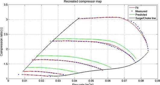
Figure 2.13 Graph of the recreated compressor flow map with fitted and

predicted curves. 45

Figure 2.14 Low speed area of the compressor 46

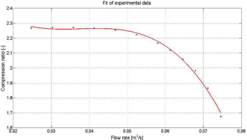
Figure 2.15 Example of a third order fit of a compressor flow curve 46 Figure 2.16 Fitted and extrapolate compressor flow curves in the low

speed area 47

(7)

Figure 2.18 Fitted power curves 48 Figure 2.19 Fit of coefficient b1 as function of the Mach number 49 Figure 2.20 Fitted and extrapolated compressor efficiency curve in the

low speed area 50

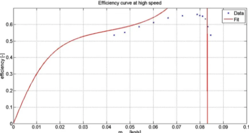
Figure 2.21 Fitted compressor efficiency curve in the high speed area 50

Figure 2.22 Simulated compressor map 51

Figure 2.23 Turbine maps from the manufacturer 52 Figure 2.24 Fitted and predicted turbine efficiency curves 53 Figure 2.25 A second order fit of turbine flow maps is used to estimate a

maximum reduced mass flow rate. An extra data point is created by fixing this maximum value to a high expansion ratio 55

Figure 1.31 Fitted turbine flow curves 56

Figure 2.27 Comparison between measured and predicted in-cylinder pressure. Engine speed=1500 rpm, BMEP=13 bar, EGR=0% 58 Figure 2.28 Comparison between measured and predicted heat release

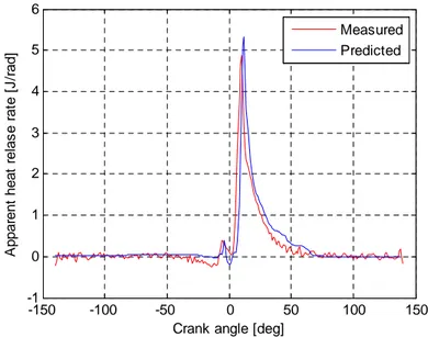
rate. Engine speed=1500 rpm, BMEP=13 bar, EGR=0% 59 Figure 2.29 Comparison between measured and predicted in-cylinder

pressure. Engine speed=2000 rpm, BMEP=13 bar, EGR=12% 59 Figure 2.30 Comparison between measured and predicted heat release

rate. Engine speed=3000 rpm, BMEP=4 bar, EGR=30% 62 Figure 2.35 Comparison between measured and predicted Indicated mean

Effective Pressure (IMEP) for the whole set of experimental data.

(8)

Figure 2.36 Comparison between measured and predicted turbine inlet

temperature. R2=0.9964 63

Figure 2.37 Optimization results: NO engine emissions in case of base

and optimal control variables 66

Figure 2.38 Optimization results: EGR rate in case of base and optimal

control variables 66

Figure 2.39 Optimization results: SOI for the main injection engine emissions in case of base and optimal control variables 67 Figure 2.40 Optimization results: Soot emissions in case of base and

optimal control variables 67

Figure 3.1 Scheme of the engine model developed in GT-Power®. The red arrows indicate the model input variables supplied by the Matlab/Simulink environment in the co-simulation process 72 Figure 3.2 Cooled low pressure EGR system on the CGN engine 74 Figure 3.3 Predicted and experimental burned fuel fraction vs. engine

crank angle. Engine speed=11000 rpm, brake torque=640 Nm, EGR

rate=20% 76

Figure 3.4 Predicted and experimental burned fuel fraction vs. engine crank angle. Engine speed=1500 rpm, brake torque=850 Nm, EGR

rate=7% 76

rate=0% 77

rate=13% 77

Figure 3.7 Comparison between measured and predicted boost pressure in the 12 operating conditions considered for model validation.

R=0.989 79

Figure 3.8 Comparison between measured and predicted brake torque in the 12 operating conditions considered for model validation.

(9)

Figure 3.9 Measured and predicted in-cylinder pressure vs. Engine crank angle. Engine speed=1100 rpm, brake torque=850 Nm, EGR

rate=0% 80

Figure 3.10 Measured and predicted in-cylinder pressure vs. engine crank angle. Engine speed=1100 rpm, brake torque=850 Nm, EGR

rate=13% 80

rate=0% 81

rate=13% 81

Figure 3.13 Estimation of the TLF at full load without EGR vs. engine

speed 83

Figure 3.14 Load-speed map of the operating conditions considered as

test cases for the optimization analysis 84

Figure 3.15 Scheme of the co-simulation process 85 Figure 3.16 Optimization results: normalized TLF in case of base (no

EGR) and optimal control variables 86

Figure 3.17 Optimization results: Brake Specific Fuel Consumption in case of base (no EGR) and optimal control variables 86 Figure 3.18 Optimization results: EGR rate in case of optimal control

variables 87

Figure 3.19 Optimization results: Spark advance in case of base (no EGR)

and optimal control variables 87

Figure 3.20 Optimization results: Waste-gate valve opening in case of base (no EGR) and optimal control variables 88 Figure 4.1 Effect of voltage disturbance on actuator chamber pressure and

wastegate valve position 90

Figure 4.2 Top view of MVEN library. This top view shows the components that are utilized and reused when building engine

(10)

Figure 4.3 Mean Value Engine Model for a two stage turbocharger engine 93 Figure 4.4 Two stage turbocharging system sketch. LPC, HPC, BP, SV,

IC, TH, HPT, LPT, WG and CAT mean respectively low pressure compressor, high pressure compressor, by-pass, surge valve, intercooler, throttle, high pressure turbine, low pressure turbine,

wastegate and catalyst 95

Figure 4.5 Wastegate position control system scheme: the blue line represents the electrical signal, the red lines represent the pipe connections and the direction of the mass flow. The components are

not to scale 96

Figure 4.6 Actuator working principle and forces acting on the

mechanical system 96

Figure 4.7 Plunger movement inside solenoid valve for the three possible working position. The plunger is drawn in blue color while the component drawn whit squared black-white at extremities of the

figure is the solenoid 97

Figure 4.8 Influence of PWM signal on leakage discharge coefficient

(upper) and actuator pressure (lower) 101

Figure 4.9 Identification of hysteresis phenomenon with a up-down slow

ramp in PWM signal 102

Figure 4.10 Influence of force of the exhaust gases with constant PWM

signal 103

Figure 4.11 Spring stiffness 103

Figure 4.12 Validation of the model. The pressure lines represent: measured actuator pressure (black solid), model actuator pressure (red dashed), measured tank pressure (blue solid) and model tank pressure (light blue dashed). In the actuator position plot, the measured position is in blue solid and the calculated position is in

red dashed 105

Figure 4.13 Compensator performance for the supply voltage disturbance. The second plot shows the wastegate position without compensator

(11)

Figure 4.14 Comparison between two different control strategies for low engine speed. HP-wastegate is controlled keeping respectively LP-wastegate fully closed (solid) and fully opened (dashed) 107

Figure 4.15 Control system structure 108

Figure 4.16 Performance of the control system at 1500 rpm subject to steps in reference value with a constant supply voltage. Upper plot: reference (solid) and actual pressure (dashed) are drawn. Lower:

Corresponding PWM signal 110

Figure 4.17 Performance of the control system with the developed compensator at 1500 rpm and a pressure set-point of 125 kPa. Upper plot: System voltage. Lower plot: PWM signal (black solid), desired (blue solid) and current (red dashed) boost pressure 111

(12)

Index of tables

Table 2.1 Acronyms of Figure 2.5 29

Table 2.2 Data sheet of the reference engine 57

Table 2.3 Operating conditions selected as test cases for the optimization

analysis 64

Table 3.1 Data sheet of the reference engine 73

Table 3.2 Coefficients of the polynomial regressions for the estimation of

parameters n, a and θb 75

(13)

1.

CHAPTER 1 Introduction

Combustion engines have been for a long time the most important prime mover for transportation globally. A combustion engine is simple in its nature; a mix of fuel and air is combusted, and work is produced in the operating cycle. The amount of combusted air and fuel controls the amount of work the engine produces.Equation Chapter 1 Section 1

The engine work has to overcome friction and pumping losses, and a smaller engine has smaller losses and is therefore more efficient. Increasing engine efficiency in this way is commonly referred to as downsizing. Downsizing has an important disadvantage; a smaller engine cannot take in as much air and fuel as a larger one, and is therefore less powerful, which can lead to less customer acceptance.

By increasing the charge density the smaller engine can be given the power of a larger engine, and regain customer acceptance. A number of charging systems can be used for automotive application, e.g. supercharging, pressure wave charging or turbocharging. Turbocharging has become the most commonly used charging system, since it is a reliable and robust system, that utilizes some of the energy in exhaust gas, otherwise lost to the surroundings.

There are however some drawbacks and limits of a turbocharger. The compressor of a single stage turbo system is sized after the maximum engine power, which is tightly coupled to the maximum mass flow. The mass flow range of a compressor is limited, which imposes limits on the pressure build up for small mass flows and thereby engine torque at low engine speed. Further, a turbo needs to spin with high rotational speed to increase air density, and due to the turbo inertia it takes time to spin up the turbo. This means that the torque response of a turbocharged engine is slower than an equally powerful naturally aspirated engine, which also lead to less customer acceptance

A two stage turbo system combines two different sized turbo units, where the low mass flow range of the smaller unit, means that pressure can be increased for smaller mass flows. Further, due to the smaller

(14)

inertia of the smaller unit, it can be spun up faster and thereby speed up the torque response of the engine. The smaller unit can then be bypassed for larger mass flows, where instead the larger turbo unit is used to supply the charge density needed [71].

1.1 Generalities on engine modeling

In the past years, the recourse to experimental analyses on the test bench was the only way to design an engine, analyze the pollutant emissions and develop engine control strategies. This method laid heavy in terms of human resources, facilities and time and, then, on the development costs. These aspects influenced both the final cost on the customer and the product time-to-market.

Starting from the need of limiting time and costs, the engine models have been developed to estimate engine performances and pollutant emissions with a narrow set of experimental data. The use of mathematical models in an automotive control system is gaining increased interest from the industry. This increased interest comes from the complex engine concepts used, where additional actuators and degrees of freedom are added to the systems. Model based control is proposed as a way of handling the increased complexity.

According to the description of phenomenon, the use of experimental data and computational time, the models can be classified into:

• White box

• Grey box

• Black box

The white box models are based on the resolution of partial differential equations (PDE) and the need of experimental data is very limited. This means that the white box models are untied from engine geometry and characteristic with an high degree of generalization. The drawback is the high computational effort, therefore only steady state condition can be simulated with these kind of models.

The black box models use a large number of experimental data in order to make up to the lack of a physical mathematical description. The benefit of the black box models is the limited computational demand.

(15)

Thank to this peculiarity, they are suitable for real-time applications such as on-board and ECU implementation.

The gray box models are the right settlement between the generalization of white box models and the fast computational time of black box models: they merge the experimental and physical information about the process. They are frequently used for the engine control tuning, assumed a given geometry.

The choice about the model to be used derives from the kind of engine under test. Indeed the most critical phenomena to model are different depending on the fuel, the modality of combustion and the presence of the turbocharger.

For a compression ignition engine (CI), especially for a Common Rail multiple injection Diesel engine, the attention has to be focused on the combustion phase and on the in-cylinder events because they are the most critical phenomena in the engine cycle. The reason consist in the modality of the mixture formation. Almost all the modern Diesel engines adopt the direct injection: the fuel is injected directly in the combustion chamber and the air turbulence has to provide the sufficient energy for the mixture before reaching the flammability conditions. In a Multijet engine, there are several injection per engine cycle (till 8 per cycle in the Multijet II system). The first interesting effect is that the composition in the combustion chamber cannot be considered homogeneous. Furthermore the ignition timing cannot be decided and determined a priori. It is evident that, in order to have a good estimation of the engine cycle, the phenomena above described must be modeled with an high degree of physical concepts.

In a spark ignition engine (SI) with indirect fuel injection, the combustion is easiest to simulate because the mixture come in the combustion chamber already mixed and its composition can be assumed homogenous. Besides the combustion starts depending on the sparking plug timing. The most common used combustion models are based on quasi-dimensional approach, with semi-empirical Wiebe law for the heat release rate simulation. For these engines the inertia and dynamic effects in intake and exhaust systems have greater influence. One-dimensional models of gas dynamics, representing the flow and the heat transfer in the piping and in the other components of the engine system are often used for SI engine simulation.

(16)

(mostly turbochargers) also to smaller engines equipping the city cars. This justifies the increasing interest of manufacturers about turbochargers and the development of a wide numbers of turbocharger models.

1.2 Combustion modeling

The combustion models can be divided in three categories: zero-dimensional models, quasi-zero-dimensional models and multi-zero-dimensional models [19][33][88][98].

The zero-dimensional models or single zone models suppose that at any time the composition and the temperature of the in-cylinder gases are uniform. These kind of models are able to forecast very well the performances of the engine with a low computational effort as shown in [8][14][17][18][113]. Nevertheless they are not suitable for the estimating of the gradients of gas composition and temperature in the combustion chamber, which are fundamentals for the pollutant emissions calculation.

In opposition to the zero-dimensional models, there are the multi-dimensional models, in which the differential equations, that describe the in-cylinder fluid motion, are solved by using very fine grids. However, some processes are still simulated by means of phenomenological submodels and the simulation results are strongly influenced by the used calibration parameters. Consequently, it is not possible guarantee for each operating condition an adequate level of accuracy. In addition, the computational time and memory request impose the application only for the design of the combustion chamber and not for the definition of control strategies.

In the middle there are the quasi-dimensional models. They combine the benefit of both types of models, through the resolution of balance equations of mass and energy without explicitly integrating the balance equations of momentum. These models are able to provide information about the spatial distribution of temperature and composition of in-cylinder gases with lower detail than multi-dimensional but with a much lower computational burden. Over the years several quasi-dimensional models have been developed with only two zones ([7] e [91]) up to models with more than one hundred zones ([63], [14], [70] e [86]). These models, as well as the number of zone, differ in the level of detail and

(17)

accuracy of the submodels used in the description of processes of penetration, atomization, evaporation, mixing and combustion. Some multi-zone models simulate the mixing and subsequent burning without considering the dynamics of the spray ([68] e [77]). For example, in [68], an instantaneous vaporization of the fuel injected into the cylinder is assumed. Other models, such as that proposed in [77], consider the processes of atomization and evaporation so rapid compared to the mixing that can be neglected: the spray is described as a jet of steam and the liquid phase is not considered. Strictly speaking, the processes of atomization and evaporation can be neglected only if the in-cylinder conditions are close to the fuel critical point. Therefore, it is not possible to apply this type of models in a wide range of engine operation. One of the most advanced multi-zone models is undoubtedly the one proposed by Hiroyasu and Katoda ([63]) and later taken by Jung and Assanis ([67]), where the spray is divided into many zones, both along the axial and radial direction, simulating the time evolution of each of them. The angle formed at the base of the spray penetration, the Sauter mean diameter and the breakup length are simulated using experimental correlations obtained through studies in environments with constant pressure. In addition, the effect of swirl motion and the collision of the jet with the cylinder walls is considered through appropriate empirical coefficients. An important point has to be taken in account: in the latest generation of Diesel engines, the fuel injection pressure and the in-cylinder pressure and temperature at the time of injection are significantly higher than those considered in these models. It should be noted that among the mentioned multi-zone models, there are few examples of combustion submodels that can simulate adequately both the diffusive and premixed combustion. For example, in the model proposed in of Ramos J. I.[92], the burning rate depends on the amount of air incorporated during the premixed combustion without taking into account the mixing. Many works, as [63] and [118], assume that the fuel burns in a stoichiometric mixture. These models overestimate the temperature in the combustion chamber and therefore overestimate the NOx emissions. In addition, they are extremely sensitive to the amount of

entrained air which is often calibrated appropriately through coefficients that take values very different among the different authors [67]. At last, in other works ([23]) the combustion submodel is based on a turbulent simplified approach, in order to take into account the effect that the mixing has on the combustion. Many Multi-zone models do not consider

(18)

radiative heat exchange ([63] and [118]): its contribution to the overall heat transfer may vary significantly (5 ÷ 50%) [62].

In almost all multi-zone models the emissions of NOx and SOOT are

estimated using, respectively, the well-known Zeldovich mechanism ([62]) and the formation mechanism of oxidation proposed by Hiroyasu et al. [63]. In some recent works the oxidation model proposed by Nagle and Strickland-Constable was also applied [67][88].

1.3 Turbocharger performance representation

State-of-the-art analyses on turbocharger modeling, as the one proposed in [71], evidence that turbocharger performances are usually presented through maps based on corrected variables. The corrections are important, since the performance maps are otherwise only valid for the conditions under which they were measured. The basis for the corrections is the dimensional analysis [106] and the correction equations relevant for a turbochargers are presented in [38][76][115]. The correction equations scale the turbine and compressor performance variables, based on the current inlet temperature and pressure. An experimental investigation of the correction quantities for the compressor is presented in [75]. There are standards describing the procedures involved in measuring a turbo map, see [95][96][13][31]. The definition of when surge occurs, which gives the smallest mass flow point for a corrected compressor speed, have been discussed in recent works [1][47]. A summary of some different turbocharger test facilities is presented in [47]. Methodology to measure turbo performance on an engine in a test stand is presented in [73].

1.3.1. Compressor map

There are four performance variables for the compressor map: corrected mass flow, pressure ratio, corrected shaft speed and adiabatic efficiency. The corrected compressor mass flow is given by the eq. (1.1)

(19)

01 , , 01 , c std c corr c c std T T m m p p = ɺ ɺ (1.1)

where mɺ_c is the compressor mass flow, T is the compressor inlet ₀₁

temperature, and p is the compressor inlet pressure. The temperature ₀₁

,

c std

T and the pressure p_{c std}_, are the reference states. The reference states must be supplied with the compressor map, since these states are used to correct the performance variables. The compressor pressure ratio is given by the eq. (1.2) 02 01 c p p Π = (1.2)

where p is the compressor outlet pressure. The corrected shaft speed ₀₂

is defined as eq. (1.3) , 01 , 1 c corr tc c std N N T T = (1.3)

where N is the turbo shaft speed. The adiabatic efficiency of the _tc

compressor is defined as eq. (1.4) 1 02 01 02 01 1 1 c c c p p T T γ γ η −   −     = − (1.4)

where γ_c is the ratio of specific heats for air. The adiabatic efficiency describes how efficient the compression of the gas is, compared to an ideal adiabatic process. Or in other words, how much the pressure increases, compared to how much the temperature increases. Points measured with equal N_{c co rr}_, are connected in the compressor map, and

(20)

are referred to as speed lines. A speed line consists of a number of measurements of Π_c and mɺ_{c corr}_, and gives the characteristics of the compressor. Compressor efficiency η_c is also measured for each point, and contours of constant η_c are normally superimposed over the speed lines. The mass flows measured on each speed line range from the surge line into the choke region. An example of a compressor map is shown in Figure 1.1

The surge line is the boundary of stable operation of the compressor. A compressor will enter surge if the mass flow is reduced below this point. Surge is an unstable condition, where the mass flow oscillates. These oscillations can destroy the turbo. Compressor choke is found for high mass flows, and indicates that the speed of sound is reached in some part of the compressor. Measurements are conducted at different N_{c co rr}_, up to the maximum allowable, and mechanical failure of the turbo can result if the speed is increased further.

(21)

1.3.2. Turbine map

As for the compressor map, there are four performance variables used in the turbine performance map: corrected mass flow, expansion ratio, corrected speed and adiabatic efficiency. It is further common to define two more

variables for the turbine: turbine flow parameter and turbine speed parameter. The corrected turbine mass flow is given by the eq. (1.5)

03 , , 03 , c std t corr t c std T T m m p p = ɺ ɺ (1.5)

where T_{c std}_, and p_{c std}_, can be other standards states, than are used in the compressor maps. The turbine mass flow mɺ is the combustion _t

products and thus normally the sum of fuel and air. The pressures p and ₀₃

04

p are the turbine inlet and outlet pressure, respectively, and T and ₀₃ T ₀₄

are the turbine inlet and outlet temperature, respectively. It is common to neglect the standard states in eq. (1.5), and present turbine data using the turbine flow parameter or TFP

03 03 t T TFP m p = ɺ (1.6)

The turbine expansion ratio is given by the eq. (1.7) 03 04 t p p Π = (1.7)

Some authors prefer to have the pressure after the component divided by the pressure before, as is the case for the compressor pressure ratio, as eq. (1.2). The corrected turbine shaft speed is given by the eq. (1.8)

(22)

, 03 , 1 t corr tc t std N N T T = (1.8)

It is common to neglect T in eq. (1.8) and define the turbine speed _std

parameter (TSP) as the eq. (1.9)

03

1

tc

TSP

N

T

=

(1.9)

Figure 1.2 Example of turbine map

Since p_std and T_std are constants, neglecting them in eq. (1.5) and (1.8) to give eq. (1.6) and (1.9) respectively, gives only a scaling.

The adiabatic efficiency of the turbine is given by the eq. (1.10) 03 04 1 04 03 1 1 t t t T T p p γ γ η = − ₋   −    (1.10)

where γ_t is the ratio of specific heats for the exhaust gas.

The high temperatures on the turbine side cause large heat fluxes. Measurement of T₀₄ can have substantial systematic errors, due to the heat

(23)

fluxes. An alternative efficiency definition for the turbine side is therefore commonly used, where no measurement of T₀₄ is needed. The heat transfer effects are less pronounced on the compressor side, and the compressor power

02 01

( )

c c p

P =mɺ ⋅c T −T (1.11)

can be used to define an alternative efficiency. This alternative turbine efficiency definition includes the shaft friction, and the equation is

(

)

, 02 01 1 04 , 03 03 1 t t c p c t t m t p t m c T T p m c T p γ γ

η η η

= ⋅ = ⋅ ⋅ − ₋       ⋅ ⋅ ⋅ −_   _       ɺ ɶ ɺ (1.12)

where the shaft friction is included in the mechanical efficiency η_m. Figure 1.2 shows an example of a turbine map.

1.4 Turbochargers modeling

Modeling of nominal turbochargers operation is divided into three subsections, depending on the model structure.

1.4.1. 3D and 1D models

Gas motion can be modeled in 3D, e.g. solving the Navier-Stokes equations of gas motion numerically. Such modeling needs accurate geometric information of the system, see e.g. the complex impeller geometries of Figure 1.3.

(24)

Figure 1.3 Compressor impeller

The boundary conditions of the model are further important, i.e. how the gas enters and leaves the modeled component. Due to the complexity and the computational effort, these models are most often only used to model components of the engine [119][57][60]. The solutions obtained, give valuable information of for example the gas motion, that can be used also for less complex model families. Also the reverse is true [29]; good models from less complex model structures can be used on a component level for a 3D simulation. Another level of detail that is frequently used, is the 1D model family. They model the gas flow along pipes and account for properties in this dimension. However 1D models of compressors are rarely found. The computational cost is reduced, compared to 3D models, and large parts of an engine system can be simulated with reasonably short simulation times.

1.4.2. Physical 0D compressor models

For the physical compressor model, an ideal compression process is frequently assumed, and different losses are then described and subtracted from the ideal component performance. This model structure often makes use of the velocity triangles, exemplified for the impeller entry in Figure 1.4. This section follows a gas element through the compressor, and describes important losses along the way, that are compiled to the model. The air flow into the compressor is assumed to have no circumferential velocity, i.e. no pre-whirl, and the diffuser section is assumed to be vane-less. An automotive compressor is normally vane-less and without intentional pre-whirl, due to the fact that a vaned diffuser normally has a

(25)

narrower flow range, and a pre-whirl system is avoided due to additional cost and packaging constraints.

Figure 1.4 Velocity triangle

The first losses occur since the gas has to comply with the vane geometry at the impeller inlet. These losses are referred to as incidence losses [53], and are due to that the inducer relative velocity vector W does not agree with the vector parallel to the vane surface, V, see Figure 1.4. The impeller vane angle varies with the radius of the impeller, since the outer points on the impeller have higher relative velocities [49]. Studying Figure 1.4, the incidence losses are minimized if I = 0, but [53] states that the actual velocity vectors are not given simply by the geometries of the compressor, due to inertial effects of the gas. The fluid friction losses due to the gas viscosity and motion through the compressor are modeled in [115][55][52], where slip is used to model the gas flow through the impeller. Slip describes how well the gas is guided by the impeller vanes, and is discussed and modeled in [38][76][90]. Generally, the less guidance the gas attracts from the vanes the more slip. The more guidance, the more friction. Due to the potentially large pressure gradient through the compressor, flow can recirculate unintentionally. These flow recirculation losses occur due to the clearance between the impeller, rotating at high velocity, and the compressor housing. Flow recirculates both from the pressure side of the impeller vanes to the suction side, and along the compressor housing, from after the impeller, to the impeller entry. Models of these losses are presented in [53][66].

(26)

The air that recirculates to the impeller entry, is already heated by the compression process. The temperature of the recirculated air increases with increased compressor pressure ratio, and the amount of recirculated air is a function of pressure ratio and not turbo speed. This recirculation occurs where the local gas pressure is high and velocity is low [60]. Experimental data of recirculation is also presented in the literature [1]. The radial temperature profile at the impeller entry is experimentally shown in [1]. For compressors with vaned diffusers, an incidence loss can be associated with the air leaving the impeller, and entering the diffuser passages. These losses are however not simply given by the geometries of the impeller and diffuser vanes, but also of the flow physics inside the impeller [49]. Experimental investigations of the gas motion in the diffuser is found in [97]. The main cause of the diffusion process losses, are in [38] said to be separation of boundary layers and fluid friction. Losses in the volute [114], and losses due to disc friction [116] and choking [29] can also be modeled. The losses associated with the volute are more pronounced for a vaned diffuser, and are modeled in [53]. In [66] it is noted that the relative magnitude of the clearance, backflow and volute losses decreases with increasing mass flow, since the losses associated with incidence and friction increase more.

1.4.3. Curve fitting 0D based models

The curve fitting based approach is another subset of the 0D model family, and recognizes that all performance variables are conveniently given by the speed lines and the efficiency contours of the map. The modeling effort is then to fit different curves to the map, or to a transformed map.

Semi-physical modeling usually transforms the compressor map variables into the dimensionless head parameter Ψand the dimensionless mass flow coefficient Φ. A connection between Ψ and Φ is then parameterized and used as a model [65][103][41]. Curve fitting directly to the map variables is another way to produce a model. The modeling effort is then to create functions describing the speed lines and iso-contours of efficiency of the map. A summary of curve fitting models for automotive control applications is presented in [79], and both speed line shapes [22] and efficiency contours are modeled [2][101][44]. Both the models of [72] and [74] use a parametrized ellipse to represent the speed lines of the

(27)

map, and are therefore of the curve fitting family.

1.4.4. Choke flow and restriction modeling

The previous section described nominal compressor operation and these section presents research relevant for modeling choked flow, and when the compressor only restricts the air, e.g. compressor operation with a pressure ratio lower than unity. If the inlet section of the compressor chokes, the choking is independent of compressor speed. This since the flow is choked, before it reaches the impeller blades. A varying choke mass flow with shaft speed, can be expected if choking conditions are established further into the compressor. This since the density of the gas arriving at the choking section, can be increased through an increase in compressor speed. In [52] the choke mass flow, assuming that choking occurs in the impeller, is described as an increasing function in shaft speed. A model that extrapolates compressor performance maps to smaller pressure ratios, including choking effects, is described in [29]. For pressure ratios lower than unity the compressor is assumed to work as an restriction for the flow, and the behavior of the compressor is compared to a nozzle discharge [81], where further a constant efficiency of 20 % is assumed in this operating region. [74] uses a choke mass flow model that is affine in corrected shaft speed. This is physically motivated by that a compressor impeller that stands still has a non-zero choke flow, and an increase in choke flow can be expected for increases in corrected shaft speed, up to the point where the compressor inlet chokes. The speed line model in [72] focuses on a the nominal compressor map, but the speed lines are extended to also cover pressure ratios less than unity. Constant compressor efficiency is assumed in this region in [72][74]

1.4.5. Surge and zero mass flow modeling

The last region of the compressor map is the one left of the surge line in Figure 1.1. When the compressor operating point moves beyond this line, surge will occur since the compressor is unable to maintain flow. When the flow breaks down completely, the highly pressurized air travels upstream, reversing the mass flow. This reversed flow reduces the pressure ratio, until the compressor is able to maintain positive mass flow. The pressure ratio then increases again and, if no other changes are applied to the system, the compressor enters a new surge cycle. Surge in

(28)

automotive applications can be encountered for example during a gear change in an acceleration phase. When the accelerator pedal is released, a sharp reduction in throttle mass flow results. Due to the inertia of the turbo, the compressor wheel does not slow down fast, and the compressor continues to build pressure.

To model surge many authors follow the Moore-Greitzer approach [56]. An extra state is introduced in the model to handle changes in mass flow through the compressor, where, due to the gas inertia, the compressor mass flow deviates from stationary performance curves for a transient [48]. Surge can be established from low to high turbo speeds [59]. The frequency of the surge phenomenon is mainly given by the system properties, where the downstream volume is most important. Most of the time in a surge cycle, is spent in either emptying or filling the downstream volume [47][22][56], and measurements of a clear connection between increased surge frequency and decreased downstream volume is presented in [48]. The filling period of the cycle is longer than the emptying, due to the flow through the throttle downstream of the compressor in a SI engine [56]. The surge frequency also depends on the compressor characteristic, and compressor speed will therefore also affect the surge frequency [47][56]. The surge phenomenon has a hysteresis effect, where the breakdown of the flow does not follow the same path in the compressor map as the build up of flow [1][56]. Mass flow measurements of surge presented in [1], show that the flow reversal is conducted at nearly constant pressure, followed by an increasing mass flow at lower pressure, and finally a rapidly increasing mass flow to a steady flow compressor speed line. The unstable branch of a compressor speed line is modeled using a third order polynomial, and is said to influence the modeled surge cycles to a small degree, since the time spent there is small [59]. Compressor pressure ratio at zero mass flow has been modeled in different versions in [48][107][54]. The negative flow branch of an extended compressor map, is modeled using a parabola with good accuracy in [59]. The Moore-Greitzer approach is followed in [72]and [74], and a third order polynomial in corrected mass flow is used in both papers for the unstable branch. This polynomial is parametrized to give zero derivative for the zero mass flow pressure build up point. The model of [74] then uses a turbine flow characteristic for the negative flow branch, while [74] uses the third order polynomial also for reversed flow. Constant compressor efficiency is assumed for surging mass flows in

(29)

[72][74].

1.5 Summary

The present manuscript is divided in three macro-areas concerning modeling, optimization and control of engines and components.

In the next chapter the optimization of the control variables for a turbocharged CI engine is faced [3]. The optimization analysis is based on an engine simulation model, composed of a control oriented model of turbocharger integrated with a predictive multi-zone combustion model, which allows accounting for the impact of control variables on engine performance, NOx and soot emissions and turbine outlet temperature. This

latter strongly affects conversion efficiency of after treatment devices therefore its estimation is of great interest for both control and simulation of tailpipe emissions. The proposed modeling structure is aimed to support the engine control design for common-rail turbocharged Diesel engines with multiple injections, where the large number of control parameters requires a large experimental tuning effort. Nevertheless, the complex interaction of injection pattern on combustion process makes black box engine modeling not enough accurate and a more detailed physical model has to be included in the loop. An hybrid modeling approach, composed of black and grey box models is implemented to simulate compressor flow and efficiency maps. The grey box model is used at low engine speeds while the black box model, based on a moving least squares method, provides compressor data at medium- high speed. Both models appear to perform best in their respective area. On the other hand a classical grey box approach is implemented for the turbine, along its overall working range. Compressor and turbine models are implemented in a computational scheme for integration with a predictive multi-zone combustion model that simulates the fuel jet and its interaction with surrounding gases by dividing the jet core into many parcels in order to describe the thermal gradient and the chemical composition within the combustion chamber. The whole engine model allows simulating in-cylinder pressure and temperature, NO and soot emissions as well as turbine outlet temperature, depending on engine control variables (i.e. injection pattern, Exhaust Gas Recirculation - EGR, Variable Geometry

(30)

Turbine - VGT). Model validation is carried out by comparing simulated in-cylinder pressure trace and exhaust temperature with a wide set of experimental data, measured at the test bench in steady-state conditions on a small automotive Diesel engine. In the paper the overall modeling approach is presented with a detailed description of in-cylinder, compressor and turbine models and the results of the experimental validation vs. measured data are shown. Furthermore, the optimization results over a set of operating points selected among those of interest for the ECE-EUDC test driving cycle are presented and discussed.

The third chapter deals with the impact of alternative fuels on engine control strategies [5][4]. Internal combustion engines for vehicle propulsion are more and more sophisticated due to increasingly restrictive environmental regulations. In case of heavy-duty engines, Compressed Natural Gas (CNG) fueling coupled with Three Way Catalyst (TWC) and Exhaust Gas Recirculation (EGR) can help in meeting the imposed emission limits and preventing from thermal stress of engine components. To cope with the new issues associated with the more complex hardware and to improve powertrain performance and reliability and after-treatment efficiency, the engine control strategies must be reformulated. The paper focuses on the steady-state optimization of control parameters for a heavy-duty engine fueled by CNG and equipped with turbocharger and EGR. The optimization analysis is carried out to design EGR, spark timing and wastegate control, aimed at increasing fuel economy while reducing in-cylinder temperature to prevent from thermal stress of engine components. The engine is modeled by a 1-D commercial fluid-dynamic code for the simulation of intake and exhaust gas flow arrangement. In order to speed-up the computational time, an empirical formulation based on the classical Wiebe function simulates the combustion process. Furthermore, an intensive identification analysis is performed to correlate Wiebe model parameters to engine operation and guarantee model accuracy and generalization even in case of high EGR rate. The optimization analysis is carried out by means of a co-simulation process in which the 1-D engine model is interfaced with a constrained minimization algorithm developed in the Matlab/Simulink® environment. Modeling approach and identification analysis are presented and the results of the experimental validation vs. measured data at the test bench are shown.

(31)

with turbocharger control through wastegate or VGT (Variable Geometry Turbocharger) actuation. The fourth chapter concerns with turbocharger control. Particularly a model-based design of a PID controller for the boost pressure by means of an actuation systems acting on the turbine wastegate valves is handled [34][110]. Actuation systems for automotive boost control incorporate a vacuum tank and PWM controlled vacuum valves to increase the boosting system flexibility. Physical models for the actuator system are constructed using measurement data from a dynamometer with an SI GM 2.0 liters engine having a two stage turbo system. The actuator model is integrated in a complete Mean Value Engine Model and a boost pressure controller is constructed. Based on the actuator model a nonlinear compensator, capable of rejecting disturbances from system voltage, is developed. A boost pressure controller is developed for the vacuum actuator and engine, using IMC. The complete controller is evaluated in an engine test cell where its performances are quantified and system voltage disturbance rejection is demonstrated.

(32)

(33)

2.

CHAPTER 2 Turbocharged CI engine

The interest in Diesel engines for automotive application has dramatically grown in the last decade, due to the benefits gained with the introduction of common-rail system. A strong increase in fuel economy and a remarkable reduction of emissions and combustion noise have been achieved, thanks to both optimized fuelling strategy and improved fuel injection technology. Namely, the improvement of injector time response, injection pressure and nozzle characteristics have made feasible the operation of multiple injections and have enhanced the fuel atomization. Altogether these benefits make the combustion cleaner and more efficient, thus reducing both particulate emissions and fuel consumption. Furthermore, the presence of early pilot and pre injection may enable the occurrence of a quasi-homogeneous combustion with a reduction of noise and main combustion temperature and with a decrease of NOx emissions.

Despite the technological improvements of fuel injection systems and the increase of electromechanical actuators (e.g. EGR, VGT, waste-gate) the engine control design process evidences a methodological gap of Diesel engine compared to SI engine. Nowadays the design of SI engine control is supported by complex computational architectures (i.e. Hardware-In-the-Loop, optimization, rapid prototyping) where the main features are compliant with the opposite requisites of high accuracy and limited computational demand. In the field of electronic control for Diesel engines, it is likely to expect the implementation of methodologies derived from the SI engine in order to gain all the potential benefits of the common-rail system. Massive use of advanced mathematical models to simulate powertrain and system components (mechanical and electronic devices) is needed to speed up the design and optimization of engine control strategies. This problem is particularly felt in presence of a large number of control parameters (i.e. injection pattern, EGR, VGT), as it is the case of current Diesel engines, where the exclusive recourse to the experiments is extremely expensive in terms of money and time. The complexity of Diesel engine combustion, which is governed by the

(34)

turbulent fuel-air-mixing, causes an unresolved trade-off between computational time and accuracy. Single zone models based on empirical heat release laws [17], largely used to simulate SI engine performance and emissions, are inadequate to simulate the heterogeneous character of Diesel combustion. This problem is particularly felt for emissions prediction; in that case a huge effort has to be spent for the identification analysis to reach a satisfactory accuracy. Therefore, in order to achieve suitable precision, most of the studies in the field of Diesel Engine modeling have been addressed to the basic phenomena involved into fuel injection/evaporation, air entrainment, combustion and emission formation, with particular emphasis on particulate matter (mainly soot). On the other hand many advanced models are available in the literature, based on the complete 3D description of turbulent, multi-phase flow field inside the cylinder [88][33][98]. Despite their accuracy, these models present a large computational demand and are indeed oriented to engine design (combustion chamber shaping, fuel jet/air interaction, swirl) rather than to control design application. As experienced for the SI engine control design [9], the implementation of fast and flexible models of reduced order is required. The proper solution can be found in a modular approach from single zone toward more physical multi-zone models. These models are coupled with algebraic relationships (i.e. regressions) to relate model parameters to engine state variables on the whole working range. Phenomenological two-zone or multi-zone combustion models have been proposed in literature to meet the requirements for engine control design. Such models are accurate enough to predict fuel evaporation, air entrainment, fuel-air distribution and thermal stratification with a reasonable computational demand [70][6]. Particularly, the recourse to two-zone models, coupled with a detailed identification analysis of the main model parameters, makes it possible to have a predictive tool for simulating, with a reduced computational burden, the effects of control injection variables on combustion process and exhaust emissions formation [91][12]. The interaction of in-cylinder processes with intake/exhaust systems is simulated by coupling the predictive multi-zone model with a control-oriented turbocharger model. Particularly a quasi-steady approach based on the related characteristic curves has been followed to simulate compressor and turbine, according with the methodology usually proposed in literature for control-oriented application [80][27][28]. Simulation of intake/exhaust processes allows

(35)

predicting the gas temperature downstream the turbine which has great influence on the conversion efficiency of the after-treatment devices and consequently on tail pipe emissions.Equation Chapter (Next) Section 1

2.1.1. Model structure

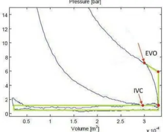
The model structure is composed of a multi-zone phenomenological model for in-cylinder pressure and temperature simulation coupled with black-box and grey box models to simulate the steady-state behavior of turbine and compressor. The interaction between in-cylinder and turbocharger models is sketched in Figure.2.1 where a scheme of the overall computational structure is shown. The external inputs are the engine speed (N) and the control variables: injection pattern, EGR rate and VGT rack position (ξ). In steady state operation, the mutual interaction of compressor and turbine models is considered through the power balance at the turbocharger shaft. In order to calculate temperature and pressure into the exhaust manifold from in-cylinder data at Exhaust valve Opening (EVO), the assumption of ideal four stroke process with constant pressure turbocharging is considered to model the open valve cycle from EVO to Intake Valve Closing (IVC) [45].

Figure.2.1 Scheme of the overall model structure, including in-cylinder, turbine and compressor models

Figure 2.2 shows the superposition of indicated and ideal exhaust

Power balance at turbocharger shaft Ideal open valve cycle

EVO IVC COMPRESSOR TURBINE IN-CYLINDER MODEL V λ C β N, inj, EGR ξξξξ TEVO pEVO NT_C ηC ηT a mɺ T mɺ pin_T Tin_T

(36)

process, evidencing the isentropic expansion at Bottom Dead Center (BDC).The former assumption simplifies the evaluation of gas properties (i.e. pressure and temperature) during the exhaust process, thus reducing the computational time with respect to the simulation of the real exhaust blowdown process. Therefore the gas is supposed to continue its expansion from EVO to BDC with the same thermodynamic law as before EVO. The characteristic parameters (i.e. polytropic data) of the expansion process are computed from the simulated pressure cycle.

Figure 2.2 Superposition of indicated and ideal intake/exhaust strokes from EVO to IVC

At BDC it is assumed that the gas expands adiabatically and its properties are computed again with common thermodynamic laws. During the exhaust stroke, the adiabatic constant pressure assumption is considered to evaluate the temperature, which remains constants from BDC to TDC. In the next sections a satisfactory comparison with experimental data is provided for the temperature estimated at turbine inlet. During intake stroke the constant pressure process is assumed and the first law of thermodynamics is exploited to compute inlet temperature and gas density at IVC [45]. Again a comparison between simulated and measured intake variables was performed with satisfactory agreement, thus guaranteeing the proper accuracy of the exhaust/intake submodel.

It is worth reminding that the assumptions made are consistent with the turbocharged Mean Value Engine Model approach for steady-state

(37)

operating condition simulation [80][27]. Such an approach is well suited for the purpose, thus solving effectively the trade-off between accuracy and computing speed.

2.2 Common-rail injector

The electro-injector is the heart of the common-rail multiple injection system and its scheme is shown in Figure 2.3. It is fed by a single high pressure fuel line which is divided in two parts. The largest amount of fuel goes to the nozzle and the smallest attends to control the rod. Both parts are used to oil the internal moving connection of the element. The injector can be divided in two main parts:

• the atomizer composed by spin and nozzle;

• the solenoid valve controller.

The control volume (Vc) (see Figure 2.3) is permanently fed with the fuel by means of the hole Z, while the discharge of the fuel is left to the hole A, controlled by the solenoid valve. The force acting on the pressure rod is proportional to the pressure ruling in the Vc. The dynamics of the pressure rod depends mainly by the equilibrium of the following forces:

• Fe: acting in closing direction due to the spring on the spin.

• Fc: acting in closing direction due to the pressure of the fuel in the

control volume at the top of the spin

• Fa: acting in opening direction due to the pressure of the fuel in the

control volume on the anchor

When the solenoid valve is not excited (see left-hand of Figure 2.3), the pressure in the atomizer and in the control volume are equal and corresponds to the rail pressure so that F_c+F_e >F_a. In this case the closing forces are greater than the opening force and the injector keep closed. In order to open the injector, the condition F_c+F_e <F_a has to be satisfied. In this case the lack of balance on the spin causes the nozzle opening and the injection of the fuel (right-hand of Figure 2.4).

(38)

Figure 2.3 Scheme of the common-rail injector [32]

The solenoid valve throws off the forces. In resting position the solenoid is not excited and the valve is closed by means of a spring. In the control volume, fed by the hole Z, there is the rail pressure and then the closing forces (Fc+Fe) are greater than the opening force (Fa). For this

conditions, there is no injection of fuel in the cylinder. By exciting the solenoid valve, the raising of the anchor is obtained, allowing the ball

(39)

valve to open the hole A. This hole has a discharge diameter greater than that of hole Z, and then the control volume empties.

Figure 2.4 Injector in closing and opening position [32]

This generates a pressure drop in the control volume that causes a decrease in the force Fc. When the force drop verifies the inequality

c e a

F +F <F , the rod begins to raise causing the opening of the atomizer. In this condition the fuel injection starts. The stop in the solenoid alimentation causes the closing of the hole A and a fast increasing of the control volume pressure till the equilibrium conditions for the closing of the injector. The quick movement of the rod, in order to guarantee a fast interruption of the injection, is due to a spring.

Because of the dynamics of the injector mechanical components, it is clear that there is no time synchrony between the electrical signal feeding

(40)

the solenoid valve (ET energizing time) and the opening of the injector, as shown in Figure 2.5 and in Table 2.1.

Figure 2.5 Time correlation between current, solenoid valve lift and nozzle lift

The only measurable variable for automotive application is the energizing time. This means that the correct injection timing (ISD) and the correct fuel volume injected in the cylinder cannot be measured by experimental test.

Detailed models of the dynamical behavior of the injector and possible improvement are available in literature [30][25][32]. These concern about the injector modeling from electrical features to fluid dynamic and mechanical features [25][32] and the possible improvement in order to avoid a pressure drop during the injection [30].

In par. 2.3.1 a simplified model of the injector is presented. The values of ISD and EID are estimated depending of the amount of injected fuel and the energizing time of each injection.

(41)

Table 2.1 Acronyms of Figure 2.5

ET Energizing Time

ED Energizing Delay

COD Control Valve Opening Delay CCD Control Valve Closing Delay NOD Needle Opening delay ISD Injection Start Delay NCD Needle Closing Delay IED Injection End Delay

EID Effective Injection Duration

2.3 In-cylinder simulation

Multi-zone model is structured so that a main routine interacts with a series of sub-routines for dynamic simulation of the jet, turbulence, combustion and emissions of pollutants. The combustion chamber is outlined in several zones with the same pressure but different temperature and composition. Each zone consists of a homogeneous mixture of ideal gases in chemical equilibrium. The thermodynamic properties of each area are measured as a function of pressure, temperature and composition [45]. Simulation of in-cylinder pressure is accomplished by a thermodynamic model, which is based on the energy conservation for an open system and on the volume conservation of the total combustion chamber [14][63][6][24]:

(42)

, , , i i i i j i j j i j

E

Q W

m

h

≠

= − +

ɺ

∑

×

ɺ

_ɺ

_(2.1) cyl a i i V =V +

∑

V (2.2)

where i is the current zone and j are the zones affected by mass and energy exchange. Eɺ represent the temporal variation of the current zone,

Qɺ the thermal power transmitted to current zone,

Wɺ

the mechanical power transmitted from the current zone to the piston, mɺ_{i j}_, the mass flow,

,

i j

h specific enthalpy, V_cyl the instantaneous cylinder volume and V and _a i

V the instantaneous volume of air zone and current zone.

During the compression stroke, the in-cylinder volume is filled by an homogeneous mixture of air and exhaust gases of the previous engine cycle, as shown in Figure 2.6

Figure 2.6 Scheme of the combustion chamber with air zone (a) and spray discretization in axial and radial direction

The composition is constant till the fuel injection which forms a spray for each injector hole. The spray is divided in radial and axial zones assuming that each zone has the same amount of fuel. In order to evaluate the thermal gradient each zone is divided in two more: burned and

(43)

unburned zone. The first one is an homogeneous mixture of combustion result, instead the second one is composed by an homogeneous mixture of air, vaporized fuel and exhaust gases of the previous engine cycle.

In order to complete eq. (2.1) and eq. (2.2), equations obtained from several submodels that describe physical phenomena, are used (e.g. for the injection, spray dynamic, evaporation, turbulence, ignition delay, combustion and pollutant emissions).

2.3.1. Injection

For estimating correctly the start of injection (SOI) and its duration from the electric signal sent by the ECU, an appropriate submodel has been developed by using the following equations:

1 , , inj d f inj C t V = (2.3) 2 , inj f inj t C V ET ∆ = ⋅ ⋅ (2.4)

where C and ₁ C are the model calibration constants, ₂ V_{f inj}_, is the amount of injected fuel for each injection and ET is the injector energizing time.

2.3.2. Spray dynamic

This submodel regards the position, the velocity end the momentum of each single zone in the spray. The spray model, called real from now, is based on the analysis of an ideal spray following these condition [82]:

• the density of the liquid fuel is much larger than that of the gas in which is injected;

• the velocity profile is constant along sections perpendicular to the axis;

• the injection speed is constant;

• fuel and entrained air move at the same speed;

• the jet has a conical shape;

• the velocity along the axis of the ideal jet is equal to that of the real jet;

• the momentum in each section perpendicular to the axis of the ideal jet is equal to that of the real jet.

(44)

Figure 2.7 Ideal jet reference

Considering the red hatched control surface in Figure 2.7, the following mass and momentum conservations equations can be written between a generic section x and the section where x=0:

( )

0

( ) ( )

fAf U f fAf x Uf x ρ = ρ (2.5)

( )

₂

( ) ( )

2

( ) ( )

2

0

f

A

f

U

f f

A x U x

f a

A x U x

a

ρ

₌

ρ



_



_

₊

ρ



_



_

_(2.6)

( )

a f f A x = A x −δ A x (2.7)

where δ_f is a variable parameter between 0 and 1, ρ_f the fuel density, A_f the fuel passing area, U_f the fuel velocity, ρ_a the air density, A the air passing area, _a A the passing area and U the velocity. By means of the three previous equations, the velocity of the spray, at any section, can be calculated. Starting from the velocity section by section and using the momentum conservation, the mass of entrained air is computed:

Optimization of SI and CI engine control strategies via integrated simulation of combustion and turbocharging

“Optimization of SI and CI engine control strategies via

integrated simulation of combustion and turbocharging”

Table of contents

Index of figures

Index of tables

1.

CHAPTER 1

Introduction

1.1

Generalities on engine modeling

1.2

Combustion modeling

1.3

Turbocharger performance representation

1.3.1.

Compressor map

1.3.2.

Turbine map

1

TSP

N

T

=

(

)

η η η

1.4

Turbochargers modeling

1.4.1.

3D and 1D models

1.4.2.

Physical 0D compressor models

1.4.3.

Curve fitting 0D based models

1.4.4.

Choke flow and restriction modeling

1.4.5.

Surge and zero mass flow modeling

1.5

Summary

2.

CHAPTER 2

Turbocharged CI engine

2.1.1.

Model structure

2.2

Common-rail injector

2.3

In-cylinder simulation

E

Q W

m

h

= − +

ɺ

ɺ

∑

×

ɺ

ɺ

∑

Wɺ

2.3.1.

Injection

2.3.2.

Spray dynamic

( )

( ) ( )

( )

( ) ( )

( ) ( )

0

A

U

A x U x

A x U x

ρ

=

ρ

_ɺ

₌

_

_

₊

_

_