UNIVERSITA’ DELLA CALABRIA
Dipartimento di Ingegneria Informatica, Modellistica, Elettronica e Sistemistica
Dottorato di Ricerca in
Information and Communication Engineering for Pervasive Intelligent Environments
CICLO XXIX
Efficient Incremental Algorithms
for Handling Graph Data
Settore Scientifico Disciplinare ING-INF/05
Coordinatore: Prof. Felice Crupi
Tutor: Prof. Sergio Greco
Dottorando: Ximena Quintana
blessing that He has managed to crystallize each of my goals, in
addition to his infinite goodness and love.
To my father Bolivar. For his life because he has been an
example of perseverance and sacrifice, he has been the engine
that has driven this professional achievement.
To my mother Nancy. For having supported me at all times,
for her advice, her values, for her constant motivation, but more
than anything, for her immense love.
To my sister Lorena. For all the love shown and to have been
a real support in the difficult moments; To my nephews Anthony
and Antonella who despite their young age their love has been
greater than distance and time separated.
To my grandparents Arturo, Zoila, Julio and Aurorita.
that although only one of them is not in the sky the four have
been my angels during all this time.
To my teachers Professor Sergio Greco and Cristian
Molinaro. For their great support and for promoting the
development of this professional training.
There has been a significant growth of connected data in the last decade. Enterprises that have changed the world like Google, Facebook, and Twitter share the common thread of having connected data at the center of their business. Such data can be naturally modeled as graphs.
In many current applications, graph data are huge and efficiently manag-ing them becomes a crucial issue. Furthermore, one aspect that many current graph applications share is that graphs are dynamic, that is, they are fre-quently updated. In this setting, an interesting problem is the development of incremental algorithms to maintain certain kind of information of interest when the underlying data is changed. In fact, incremental algorithms avoid the recomputation of the information of interest from scratch; rather, they tend to minimize the computational effort to update a solution by trying to identify only those pieces of information that need to be updated. In contrast, non-incremental algorithms need to recompute new solutions from scratch ev-ery time the data change, and this can be impractical when data are huge and subject to frequent updates.
In this thesis, two classical graph theory problems are considered: the maximum flow problem and the shortest path/distance problem. For both of them efficient incremental algorithms are proposed.
The maximum flow is a classical optimization problem with a wide range of applications. Nowadays, it is successfully applied in social network analysis for link spam detection, web communities identification, and others. In such applications, flow networks are used to model connections among web pages, online voting systems, web communities, P2P and other distributed systems. Thus, networks are highly dynamic.
While many efficient algorithms for the maximum flow problem have been proposed over the years, they are designed to work with static networks, and thus they need to recompute a new solution from scratch every time an update occurs. Such approaches are impractical in scenarios like the aforementioned ones, where updates are frequent.
To overcome these limitations, we propose efficient incremental algorithms for maintaining the maximum flow in dynamic networks. Our approach iden-tifies and acts only on the affected portions of the network, reducing the computational effort to update the maximum flow. We evaluate our approach on different families of datasets, comparing it against state-of-the-art algo-rithms, showing that our technique is significantly faster and can efficiently handle networks with millions of vertices and tens of millions of edges.
The second problem considered in this thesis is computing shortest paths and distances, which has a wide range of applications in social network anal-ysis [46], road networks [63], graph pattern matching [22], biological net-works [55], and many others. It is both an important task in its own right (e.g., if we want to know how close people are in a social network) and a fundamental subroutine for many advanced tasks.
For instance, in social network analysis, many significant network metrics (e.g., eccentricity, diameter, radius, and girth) and centrality measures (e.g., closeness and betweenness centrality) require knowing the shortest paths or distances for all pairs of vertices. There are many other domains where it is needed to compute the shortest paths (or distances) for all pairs of ver-tices, including bioinformatics [52] (where all-pairs shortest distances are used to analyze protein-protein interactions), planning and scheduling [51] (where finding the shortest paths for all pairs of vertices is a central task to solve binary linear constraints on events), and wireless sensor networks [15] (where different topology control algorithms need to compute the shortest paths or distances for all pairs of vertices).
Although many algorithms to solve this problem have been proposed over the years, they are designed to work in the main memory and/or with static graphs, which limits their applicability to many current applications where graphs are highly dynamic.
In this thesis, we present novel efficient incremental algorithms for main-taining all-pairs shortest paths and distances in dynamic graphs. We experi-mentally evaluate our approach on several real-world datasets, showing that it significantly outperforms current algorithms designed for the same problem. Main Contributions. As for the maximum flow problem, the main contri-butions are:
• We propose efficient incremental algorithms to maintain the maximum flow after vertex insertions/deletions and edge insertions/deletions/updates. Our algorithms are designed to effectively identify only the affected parts of the network, in order to reduce the computational effort for determining the new maximum flow.
• We provide complexity analyses.
• We report on an experimental evaluation we conducted on several families of datasets with millions of vertices and tens of millions of edges. Exper-imental results show that our approach is very efficient and outperforms state-of-the-art algorithms.
As for the shortest path/distance problem, the main contributions are: • We consider the setting where graphs and shortest paths are stored in
relational DBMSs and propose novel algorithms to incrementally main-tain all-pairs shortest paths and distances after vertex/edge insertions, deletions, and updates. The proposed approach aims at reducing the time needed to update the shortest paths by identifying only those that need to be updated (it is often the case that small changes affect only few shortest paths). To the best of our knowledge, [50] is the only disk-based approach in the literature for incrementally maintaining all-pairs shortest distances. In particular, like our approach, [50] relies on relational DBMSs.
• We experimentally compare our algorithms against [50] on five real-world datasets, showing that our approach is significantly faster. It is worth noticing that our approach is more general than [50] in that we keep track of both shortest paths and distances, while [50] maintain shortest distances only (thus, there is no information on the actual paths). Organization. The thesis is organized as follows. In Chapter 1, basic concepts and notations on relational and graph databases are introduced.
In Chapter 2, the incremental maintenance of the maximum flow in dy-namic flow networks is addressed.
In Chapter 3, the incremental maintenance of all-pairs shortest paths (and distances) in dynamic graphs is addressed.
Finally, conclusions are drawn.
Rende, Ximena Quintana
1 Relational and Graph Databases . . . 1
1.1 Relational Databases . . . 1
1.2 Graph Databases . . . 2
1.2.1 Neo4j . . . 3
1.2.2 OrientDB . . . 8
2 Incremental Maintenance of the Maximum Flow . . . 13
2.1 Introduction . . . 13
2.2 Related Work . . . 14
2.3 Preliminaries . . . 15
2.4 Incremental Maximum Flow Computation . . . 16
2.4.1 Edge Insertions and Capacity Increases . . . 17
2.4.2 Edge Deletions and Capacity Decreases . . . 21
2.5 Experimental Evaluation . . . 24
2.6 Discussion . . . 26
3 Incremental Maintenance of All-Pairs Shortest Paths in Relational DBMSs . . . 27
3.1 Introduction . . . 27
3.2 Related Work . . . 28
3.3 Preliminaries . . . 31
3.4 Incremental Maintenance of All-Pairs Shortest Paths . . . 33
3.4.1 Edge Insertion . . . 34
3.4.2 Edge Deletion . . . 39
3.4.3 Edge Update . . . 47
3.5 Experimental Evaluation . . . 47
3.5.1 Experimental Setup . . . 48
3.5.2 Results on the DIMES Dataset . . . 50
3.5.3 Results on the RNNA Dataset . . . 51
3.5.4 Results on the Twitter Dataset . . . 51
3.5.6 Results on the Instagram Dataset . . . 52
3.5.7 Experimental conclusions . . . 53
3.6 Discussion . . . 53
Conclusions . . . 55
Relational and Graph Databases
A database is a set of data belonging to the same context and stored sys-tematically. Database Management Systems (DBMSs) allow us to store and then access the data. Data can be structured according to different data mod-els. This chapter briefly recalls the basics of relational databases and graph databases.
1.1 Relational Databases
The existence of alphabets of relation symbols and attribute symbols is as-sumed. The domain of an attribute A is denoted by Dom(A). The database domain is denoted by Dom. A relation schema is of the form r(A1, . . . , Am)
where r is a relation symbol and the Ai’s are attribute symbols (we denote the
previous relation schema also as r(U ), where U = {A1, . . . , Am}). A relation
instance (or simply relation) R over r(U ) is a subset of Dom(A1) × · · · ×
Dom(Am). Each element of R is a tuple. Given a tuple t ∈ R and a set X ⊆ U
of attributes, we denote by t[X] (resp. R[X]) the projection of t (resp. R) on X. Given the relation schemata r(U ), s(V ), . . . we will refer to their respective instances as R, S, . . . . A database schema DS is a set {r1(U1), . . . , rn(Un)} of
relation schemata. A database instance (or simply database) DB over DS is a set {R1, . . . , Rn} where each Ri is a relation over ri(Ui), i = 1..n. The set
of constants appearing in DB will be called active domain of DB. In the following, we will also refer to the instance of the relation r in a database DB as DB[r].
A conjunctive query Q is of the form ∃Y Φ(X, Y ) where Φ is a conjunction of atoms (an atom is of the form p(t1, . . . , tn) where p is a relation symbol
and each ti is a term, that is a constant or a variable), X and Y are sets of
variables with X being the set of free variables of Q. The result of applying Q over a database DB is denoted by Q(DB).
Integrity constraints express semantic information about data, i.e. rela-tionships that should hold among data. They are mainly used to validate database transactions.
Given a relation schema r(U ), a functional dependency f d over r(U ) is of the form X → Y , where X, Y ⊆ U . If Y is a single attribute, the func-tional dependency is said to be in standard form whereas if Y ⊆ X then f d is trivial. A relation R over r(U ) satisfies f d, denoted as R |= f d, if ∀t1, t2 ∈ R t1[X] = t2[X] implies t1[Y ] = t2[Y ] (we also say that R is
con-sistent w.r.t. f d). A key dependency is a functional dependency of the form X → U . Given a set F D of functional dependencies, a key of r is a minimal set K of attributes of r s.t. F D entails K → U . Each attribute in K is called key attribute. A primary key of r is one designated key of r. In the following, we will refer to the functional dependencies in F D over a schema r(U ) also as F D[r].
Given two relation schemata r(U ) and s(V ), a foreign key constraint f k is of the form r(W ) ⊆ s(Z), where W ⊆ U, Z ⊆ V, |W | = |Z| and Z is a key of s (if Z is the primary key of s we call f k a primary foreign key constraint ). Two relations R and S over r(U ) and s(V ) respectively, satisfy f k if for each tuple t1∈ R there is a tuple t2∈ S such that t1[W ] = t2[Z] (we also say that
R and S are consistent w.r.t. f k).
1.2 Graph Databases
Although graph databases are a newer technology, they have had a strong development in recent years and today there is a variety of graph database systems. Graph databases use graph structures with nodes, edges, and prop-erties to represent and store data. General graph databases that can store any graph are different from specialized graph databases such as triple-stores and network databases. There are two properties of graph databases one should consider when investigating graph database technologies:
1. The underlying storage: Some graph databases use native graph stor-age that is optimized and designed for storing and managing graphs. Not all graph database technologies use native graph storage. However, some serialize the graph data into a relational database, an object oriented database, or some other general-purpose data store.
2. The processing engine: Some definitions require that a graph database use index-free adjacency, meaning that connected nodes physically point to each other in the database.
A graph database represents information as nodes of a graph and its rela-tions with the edges thereof. An illustrative example is reported in Figure 1.1. • Nodes represent entities and can be tagged with labels representing their
Fig. 1.1: Graph with properties.
• Edges express relationships and connect nodes. Significant patterns emerge when we consider the connections of nodes, properties, and edges. Note that even when edges are directed, relationships can always be navigated regardless of direction.
• Properties are pertinent information associated with nodes and edges. A simple way to comprehend graph databases is to imagine social networks. In this scenario we can imagine users as nodes and connections as edges. On a social media platform relationships between users are complex and through the application of this model one can get many kinds of relationships.
In the rest of this chapter, we discuss two popular graph database systems: Neo4j and OrientDB.
1.2.1 Neo4j
Neo4j is a graph database developed by Neo Technology, open source, and written in Java.
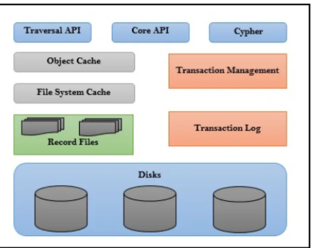
Architecture of Neo4j. Neo4j interaction can take place at various lev-els, depending on the needs of the application. Figure 1.2 shows three levels: the bottom level relative to the data storage disk, the top level that exposes functions to interact with the database, and the intermediate level contains the management system. The transactional management is optimized for graph data model.
Neo4j uses the Cypher query language to manipulate data and issue queries. Many APIs are available that allow users to make requests through Cypher. Cypher generates the execution plan, finds start node, traverse through relationships and retrieves the results. The Traversal API are of
particular interest, as they offer functionalities for graph traversal. Traver-sal happens from node to node via edges (relationships). Core API provides functionalities for initiating embedded graph databases that receive client connections. It also provides capabilities to create nodes, relationships and properties [56].
Neo4j also provides indexes. Neo4j recently introduced the concept of la-bels and their sidekick, schema indexes. Lala-bels are a way of attaching one or more simple types to nodes (and relationships), while schema indexes al-low to automatically index labelled nodes by one or more of their properties. Those indexes are then implicitly used by Cypher as secondary indexes and to infer the starting point(s) of a query. This new indexing system allows for indexing on an attribute of all nodes/relationships with a specific label and automatically maintains the index as creation, deletion, and edit updates are made.
The memory is managed efficiently through two cache, one at the level of file system that keeps the parts of files stored as records (File System cache), and a faster and higher level that keeps portions of the graph (Object Cache). Caches in Neo4j are just part of the system memory used when Neo4j instances are created and queries are being performed on those instances. Transaction Management and Transaction log keep tracks of transactional consistency and atomicity, while their record being maintained in the log. Record Files or Store Files are those where Neo4j stores the graph data. Each store file contains data for specific part of the graph (e.g nodes, relationships, properties, etc.). Some of the store files commonly seen are
• neostore.nodestore.db • neostore.relationshipstore.db • neostore.propertystore.db • neostore.propertystore.db.index • neostore.propertystore.db.strings • neostore.propertystore.db.arrays
Neo4j Features. Among the features of Neo4j there are high perfor-mance in search operations between nodes [45], the ability to adapt to the field of semantic networks [49], and the expressiveness of the query language (Cypher). For the purpose of fully maintain data integrity and ensure the proper transactional behavior, Neo4j supports the ACID properties.
For users, developers and database administrators, Neo4j provides the fol-lowing features:
• Materializing of relationships at creation time, resulting in no penalties for complex runtime queries.
• Constant time traversals for relations in the graph both in depth and in breadth due to efficient representation of nodes and relationships.
Fig. 1.2: Neo4j Architecture
• All relationships in Neo4j are equally important and fast, making it pos-sible to materialize and use new relationships later on to “shortcut” and speed up the domain data when new needs arise.
• Compact storage and memory caching for graphs.
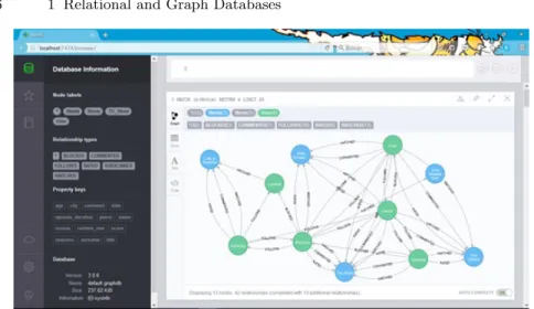
Neo4j provides a web front end for manual database querying with Cypher and for development and testing purposes, showing nodes and edges (cf. Fig-ure 1.3). The interface presents returned results by interactive graph visual-ization. On one hand it has a lightweight API that allows it to be included into Java code and run as embedded database. If it shall be used as a stan-dalone database, clients communicate via a RESTful [23] web service using an API similar to its Java API. It supports transactions also provides a user management.
Cypher. Cypher is a declarative query language. It enables one to tell what should be selected, inserted, updated, or deleted from a graph database. It is possible to run Cypher queries via CLI (Neo4j Shell), Java API, or by REST API.
The basic idea of the Cypher query language is to express patterns to be matched over the graph the user wants to query.
Nodes are enclosed by parentheses, relationships are enclosed by brackets. Nodes are connected together by –, −→ , or ←− chars.
A pattern can also match nodes and relationships with specific labels. The labels are written after the variable name separated with a colon. Nodes and relationships can be matched by their properties. Properties are written into braces as key-value pairs. Multiple properties are separated by a comma.
In the following, we briefly mention the main clauses that can be used in Cypher.
Fig. 1.3: Neo4j’s web front end.
The MATCH clause is used to express the graph pattern to match. This is the most common way to get data from the graph. A matched result set may be processed by the RETURN clause which may run a projection over the result set. Figure 1.4 shows an example of a Cypher query with MATCH and RETURN clauses in action.
Fig. 1.4: MATCH and RETURN Clauses.
The WHERE clause is inspired by SQL. Nodes and relationships can be filtered by conditions using this clause. The query in Figure 1.5 returns all name of movies that were liked by a user, but that user must not like ”The Conjuring” movie.
Cypher allows for ordering and pagination by the ORDER BY, LIMIT, and SKIP clauses.
The WITH clause allows query parts to be chained together, piping the results from one to be used as starting points or criteria in the next. Figure 1.6 reports a Cypher query limits matched paths to m node to the last one and then returns all adjacent nodes.
Fig. 1.5: WHERE Clause.
Fig. 1.6: WITH Clause.
The UNION clause combines the result of multiple queries. The UNION ALL clause is used to leave duplicates in the result set. An example is reported in Figure 1.7.
Fig. 1.7: UNION Clause.
The SET clause updates labels on nodes and properties on nodes and relationships. Setting property to the NULL removes the property. There are also ON MATCH SET and ON CREATE SET for additional control over what happens depending on whether the node was found or created, respectively. An example is reported in Figure 1.8.
The DELETE clause deletes graph elements, such as nodes, relationships or paths. As an example, the query in Figure 1.9 removes the nodes with property name Anthony and all the node’s relationships.
Fig. 1.8: SET Clause.
Fig. 1.9: DELETE Clause.
1.2.2 OrientDB
OrientDB [61] is an open source NoSQL database management system written in Java. It is a multi-model database, supporting graph, document, key/value, and object models.
The Graph Model is a data model that allows us to store data in the form of nodes connected by edges. The vertex and edge components are the central pieces of the graph model.
In the Document Model the data is stored in documents and groups of documents are called “collections”.
The Key/Value Model means that data can be stored in the form of key/value pairs where the values can be simple or complex types. It can sup-port documents and graph elements as values.
The Object Model has been inherited by object-oriented programming and supports inheritance between types, polymorphism and direct binding from/to objects.
The following terminology is used in OrientDB:
• Record. The record is the smallest unit that the system can load and store in the the database. Records can be stored as Document, Record Bytes, Vertex or Edge.
• Record ID. When OrientDB generates a record, each record has its own self-assigned unique ID within the database called Record ID or RID. The RID looks like: hcluster-idi:hcluster-positioni where hcluster-idi is the
cluster identifier and hcluster-positioni is the position of the data within the cluster.
• Documents. Documents are defined by schema classes with defined con-straints or without any schema.
• Class. The concept of class is derived from the object-oriented paradigm and it is very similar to a relational table where classes can be schema-less, complete or mixed schema. One class can inherit all attributes from another. Each class has its own grouping, although it must have at least one default cluster. When one runs a query on a class, it propagates to the cluster that is part of the same class.
• Cluster. A cluster or group is a place where the records are stored. We can compare the cluster concept to a table in the relational database model. OrientDB by default creates a cluster for each class. All the records of a class are stored in the same cluster having the same name of the class. Although the default strategy is to create a cluster for each class, a class can have multiple clusters.
• Relationships. OrientDB supports two kinds of relationships: referenced and embedded.
– Referenced relationships. The reports in OrientDB are handled natively, without making costly join performed in a relational DBMS. OrientDB stores the direct link between objects in relation to each other.
– Embedded relationships. It means it stores the relationship within the record that embeds it. This type of relationship is stronger than the reference relationship.
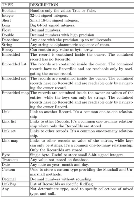
TYPE DESCRIPTION
Boolean Handles only the values True or False. Integer 32-bit signed integers.
Short Small 16-bit signed integers. Long Big 64-bit signed integers. Float Decimal numbers.
Double Decimal numbers with high precision
Date-time Any date with the precision up to milliseconds. String Any string as alphanumeric sequence of chars. Binary Can contain any value as byte array.
Embedded The record is contained inside the owner. The contained record has no RecordId.
Embedded list The records are contained inside the owner. The contained records have no RecordIds and are reachable only by navi-gating the owner record.
Embedded set The records are contained inside the owner. The contained records have no RecordId and are reachable only by navigat-ing the owner record.
Embedded map The records are contained inside the owner as values of the entries, while the keys can only be strings. The contained records have no RecordId and are reachable only by navigat-ing the owner Record.
Link Link to another Record. It’s a common one-to-one relation-ship
Link list Links to other Records. It’s a common one-to-many relation-ship where only the RecordIds are stored.
Link set Links to other records. It’s a common one-to-many relation-ship.
Link map Links to other records as value of the entries, while keys can only be strings. It’s a common one-to-many relationship. Only the RecordIds are stored.
Byte Single byte. Useful to store small 8-bit signed integers. Transient Any value not stored on database.
Date Any date as year, month and day.
Custom Used to store a custom type providing the Marshall and Un-marshall methods.
Decimal Decimal numbers without rounding. LinkBag List of RecordIds as specific RidBag.
Any Not determinate type, used to specify collections of mixed type, and null..
Table 1.1: OrientDB Data Types.
The OrientDB Console is a Java Application. OrientDB supports the fol-lowing console modes:
• Interactive Mode. This is the default mode. The Console starts in inter-active mode. We can execute commands and SQL statements, the Console loads data, and once done the console is ready to accept commands. • Batch Mode. Running the console in batch mode takes commands as
an argument or as a text file.
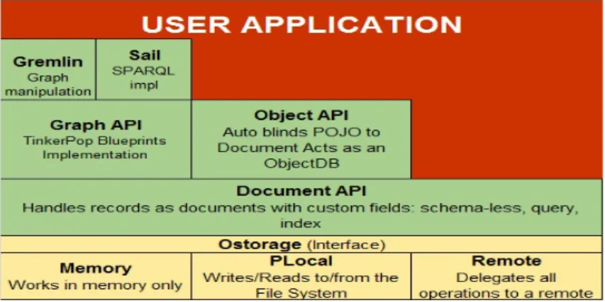
OrientDB is implemented in Java, and therefore available to a good stan-dard API for interfacing through this language. There are three models to take advantage of APIs, depending on the model with which it wants to work: Graph API, Documents API, and Object API.
• Graph API: These APIs allow one to work on graphs, one of the most flexible data structures.
• Document API: These APIs are the most immediate to use because they even match one of the most common uses of a NoSQL database. They allow you to convert Java objects into documents and save them in OrientDB.
• Object API: These APIs are based on documents and help one work with real persistent Java objects, using the reflection mechanism. The stratification of the functionality of the APIs above is represented by the following figure:
Fig. 1.10: Component Architecture.
The operations that OrientDB can perform over a database are listed below: • Create Database • Alter Database • Backup Database • Restore Database • Connect Database
• Disconnect Database • Info Database • List Database • Freeze Database • Release Database • Config Database • Export Database • Import Database • Commit Database • Rollback Database • Optimize Database • Drop Database
To handle the records OrientDB offers the following commands • Insert Record • Displays Records • Load Records • Reload Record • Export Record • Update Record • Truncate Record • Delete Record
OrientDB allows users to handle classes and cluster by means of commands to create, alter, truncate and drop.
The OrientDB commands to act on properties are: • Create Property
• Alter Property • Drop Property
The OrientDB commands to handles vertices and edges are: • Create Vertex • Move Vertex • Delete Vertex • Create Edge • Update Edge • Delete Edge
OrientDB offers also indexing mechanisms and support for transactions. Furthermore, OrientDB supports JDBC and has a Python Interface.
Incremental Maintenance of the Maximum
Flow
The maximum flow problem is a classical optimization problem with a wide range of applications. Nowadays, it is successfully applied in social network analysis for link spam detection, web communities identification, and others. In such applications, flow networks are used to model connections among web pages, online voting systems, web communities, P2P and other distributed systems. Thus, networks are highly dynamic, that is, subject to frequent up-dates.
While many efficient algorithms for the maximum flow problem have been proposed over the years, they are designed to work with static networks, and thus they need to recompute a new solution from scratch every time an update occurs. Such approaches are impractical in scenarios like the aforementioned ones, where updates are frequent.
To overcome these limitations, in this chapter we propose efficient in-cremental algorithms for maintaining the maximum flow in dynamic net-works [36, 38]. Our approach identifies and acts only on the affected portions of the network, reducing the computational effort to update the maximum flow. We evaluate our approach on different families of datasets, comparing it against state-of-the-art algorithms, showing that our technique is significantly faster and can efficiently handle networks with millions of vertices and tens of millions of edges.
2.1 Introduction
The maximum flow problem arises in settings as diverse as communication systems, image processing, scheduling, distribution planning, and many oth-ers [3, 33]. Even if the problem has a long history, revolutionary progress is still being made and the number of applications is continuously growing— e.g., see [33]. Interestingly, this problem is nowadays successfully applied in social network analysis for link spam detection [58], for the identification of web communities [25, 42], and to defend against sybil attacks [64, 62]. In such
applications, flow networks are used to model connections among web pages, online voting systems, web communities, P2P and other distributed systems. Thus, networks are highly dynamic, that is, subject to frequent updates.
Even though many efficient algorithms for the maximum flow problem have been proposed over the years, they are designed to work with static networks, and thus they need to recompute a new solution from scratch every time the network is modified. However, the aforementioned scenarios call for incremental algorithms, as it is impractical to compute a new solution from scratch every time an update occurs.
To overcome these limitations, we propose novel incremental algorithms for maintaing the maximum flow in dynamic networks.
Contributions. Specifically, we make the following main contributions: • We propose efficient incremental algorithms to maintain the maximum
flow after vertex insertions/deletions and edge insertions/deletions/updates. Our algorithms are designed to effectively identify only the affected parts of the network, in order to reduce the computational effort for determining the new maximum flow.
• We show correctness of the algorithms and provide complexity analyses. • We report on an experimental evaluation we conducted on several families
of datasets with millions of vertices and tens of millions of edges. Exper-imental results show that our approach is very efficient and outperforms state-of-the-art algorithms.
2.2 Related Work
The maximum flow problem is a classical optimization problem and many algorithms to solve it have been proposed over the years [26, 20, 21, 32, 13, 8, 48, 41, 29, 30, 9, 10, 31]. The first solutions to this problem were mainly based on finding augmenting paths in the residual network [26, 20, 21]— roughly speaking, these are paths from the source to the sink along which it is possible to send additional flow.
Approaches based on the push-relabel algorithm [32] have been proposed in [13, 29, 30]. Push-relabel algorithms do not maintain a valid flow during their execution. In particular, some vertices might have a positive flow excess. By maintaining a label for each vertex denoting a lower bound on its dis-tance to the sink along non-saturated edges, the excess is then pushed toward vertices with smaller label or, eventually, sent back to the source.
The highest-level push-relabel implementation introduced in [13], named HIPR, was for a long time a benchmark for maximum flow algorithms. Op-timizations have been introduced in the partial augment-relabel algorithm (PAR) [29]. The same data structures and heuristics of PAR are used by the two-level push-relabel algorithm (P2R) [30]. These solutions use both the
global update [32] and the gap relabeling [10] heuristics to improve the per-formance of the push-relabel method.
There are also algorithms that solve the minimum cut and the maximum flow problems without maintaining a feasible flow [41, 31]. The solution pro-posed in [41], named HPF, terminates its execution with the min-cut and a pseudoflow (which means that some vertices might have a positive or negative flow excess). However, it is possible to convert the pseudoflow into a maximum feasible flow by computing flow decomposition in a related network. As shown in [24, 10], the time spent in flow recovery is typically small compared to the time to find the min-cut.
Different from the above mentioned approaches, the algorithm of Boykov and Kolmogorov (BK) [8] has no strongly polynomial time bound. However, given its practical efficiency, it is probably the most widely used algorithm in computer vision. BK is based on augmenting paths. It builds two search trees, one from the source and the other from the sink, and reuses them.
The main limitation of all the aforementioned algorithms is that, when dealing with dynamic networks, they need to recompute a new maximum flow from scratch every time the network changes, which is impractical in applications where updates occur frequently.
Recently, some solutions have been proposed that consider the maximum flow problem in a dynamic setting [48, 31]. They mainly focus on solving a given series of maximum flow instances, each obtained from the previous one by relatively few changes in the input. The solution introduced in [48] is an extension of the BK algorithm (E-BK) to the dynamic setting. In [31], the Excesses Incremental Breadth-First Search (E-IBFS) algorithm is proposed. E-IBFS maintains a pseudoflow (like HPF), and thus an additional step has to be performed if a flow is required.
2.3 Preliminaries
In this section, we briefly recall the maximum flow problem and introduce notation and terminology used in the rest of this chapter (we refer the reader to [3] for a comprehensive treatment of the topic).
A flow network is a tuple N = (V, A, s, t, c), where
• (V, A) is a directed graph with vertex set V and edge set A;
• s and t are two distinguished vertices in V called the source and the sink, respectively;
• c is a capacity function c : A → R+ assigning a positive real capacity
c(u, v) to each edge (u, v) in A.
For convenience, we define c(u, v) = 0 for every (u, v) /∈ A, and assume that there are no self-loops.
A flow in N is a function f : V × V → R satisfying the following two properties:
• 0 ≤ f (u, v) ≤ c(u, v) for all u, v ∈ V ;
• P
v∈V
f (v, u) = P
v∈V
f (u, v) for all u ∈ V \ {s, t}.
The first property above says that the flow along an edge (u, v) cannot exceed its capacity, and the second property says that for each vertex (other than the source and the sink), its incoming flow must equal its outgoing flow.
The value of f is |f | = P
v∈V
f (v, t)−P
v∈V
f (t, v), that is, it is the net flow into the sink. The maximum flow problem consists in finding a flow of maximum value.
Given a flow f in N and two vertices u, v ∈ V , the residual capacity is defined as rf(u, v) = c(u, v) − f (u, v) + f (v, u). The residual network of N
induced by f is the directed graph Nf = (V, Ef), where Ef = {(u, v) ∈
V × V : rf(u, v) > 0}. A simple path (i.e., a path without repeating vertices)
from s to t in Nf is called an augmenting path.
2.4 Incremental Maximum Flow Computation
In this section, we present algorithms for the incremental maintenance of the maximum flow. We first propose an algorithm to handle edge insertions and capacity increases (Section 3.4.1), and then address edge deletions and capacity decreases (Section 3.4.2).
It is worth noting that insertions and deletions of vertices can be straight-forwardly reduced to our setting and thus can be handled by our algorithms too: vertex insertions (resp. deletions) are handled by inserting (deleting) all edges that are incident from/to the inserted (resp. deleted) vertices.1 As a consequence, our algorithms can handle arbitrary sequences of edge inser-tions/deletions/updates (the latter to be understood as capacity updates) and vertex insertions/deletions. Since the insertion of an edge (a, b) s.t. either a or b (or both) is a new vertex does not affect the maximum flow—i.e., the flow along (a, b) will be zero and remain the same elsewhere—we assume that both a and b belong to the current flow network.
Given a flow network N = (V, A, s, t, c), a pair of vertices (a, b) ∈ V × V , and a real value w, we use update(N, (a, b), w) to denote the flow network N0 = (V, A0, s, t, c0) such that c0 is the same as c except that c0(a, b) = max{0, c(a, b) + w} and A0 = {(u, v) ∈ V × V | c0(u, v) > 0}. Thus, when w > 0, if (a, b) ∈ A then the edge capacity is increased by w, otherwise the new edge (a, b) with capacity w is inserted into the network. When w < 0, the capacity of (a, b) is decreased by w, which corresponds to deleting the edge altogether when c0(a, b) = 0.
We start by introducing two functions which will be used by both our algorithms: ASP (Augmenting Shortest Path) and UF (Update Flow).
1
ASP takes as input a residual network Nf = (V, Ef) and two vertices
x, y ∈ V , and it returns two vertex-indexed arrays, prev and flow , containing the shortest path from x to y (if it exists) and the maximum additional flow that can be pushed along that path, respectively. Essentially, ASP performs a breadth-first search from x, and for each vertex v reached during the visit, it keeps track of the maximum additional flow (denoted flow [v]) that v can receive from x along the discovered shortest (in terms of number of edges) path connecting them, together with v’s predecessor in such a path (denoted prev [v]). If y is reached, then it is possible to build the whole path from x to y by following the chain of predecessors in prev starting from y. Otherwise (y is not reachable from x), the algorithm stops when there are no more vertices reachable from x. In the function, Q is a first-in, first-out queue. Also, we use adj [u] to denote the set of u’s adjacent vertices (in Nf).
The UF function takes as input a flow network N , a flow f in N , an additional flow value ∆f , two vertices x, y, and an array of predecessors prev (which will be computed by ASP in Algorithms 3 and 2). The function simply increases f by ∆f along the path from x to y stored in prev .
2.4.1 Edge Insertions and Capacity Increases
In this section, we present our algorithm to incrementally maintain the max-imum flow after inserting a new edge or increasing the capacity of an exiting one. Algorithm 3 takes as input a flow network N , a maximum flow f in N , an edge (a, b), and a positive capacity w, and computes a maximum flow in update(N, (a, b), w).
First of all, notice that lines 2–27 are executed only if (a, b) is a new edge or an existing one that has been used to its full capacity, because if this condition does not hold, then the insertion/update of (a, b) has no effect on the maximum flow. The algorithm works as follows. First, it computes the new flow network N (line 2). Then, it looks for a (shortest) path from s to a in the residual network by calling the ASP function (line 3). If such a path exists, an analogous search is performed from b to t (line 6). If also such a path exists, then there is an augmenting path p from s to t and the maximum flow is increased on the edges of p (lines 9–12).
After that, if (a, b) has still positive residual capacity, Algorithm 3 repeats the search of augmenting paths in Nfas follows (lines 16–27). If additional flow
can be sent from s to a along the previously discovered path, the algorithm looks for a path from b to t (lines 17–18); otherwise (no additional flow can be sent from s to a along the previously discovered path), if additional flow can be sent from b to t along the previously discovered path, the algorithm looks for a path from s to a (lines 20–21); otherwise (no more flow can be sent along the previously discovered paths), the algorithm looks for both a path from s to a and a path from b to t (lines 23–27). The search continues until either the residual capacity of (a, b) gets to zero (i.e., no more additional flow
Function 1 Augmenting Shortest Path (ASP)
Input: A residual network Nf = (V, Ef), two vertices x, y ∈ V .
Output: Arrays prev and flow . 1: flow [1..|V |]; 2: prev [1..|V |]; 3: for each v ∈ V do 4: flow [v] := −1; 5: prev [v] := NIL; 6: flow [x] := +∞; 7: if x = y then
8: return hprev , flow i; 9: Q := {x};
10: while Q 6= ∅ do 11: u := Q.dequeue();
12: for v ∈ adj [u] s.t. flow [v] = −1 do 13: flow [v] := min{flow [u], rf(u, v)}; 14: prev [v] := u;
15: if v = y then
16: return hprev , flow i; 17: Q.enqueue(v);
18: return hprev , flow i;
c 10/20 a 10/15 5/15 5/5 e b 5/5 5/5 10/15 d 10/10 S f T 20/40 0/5
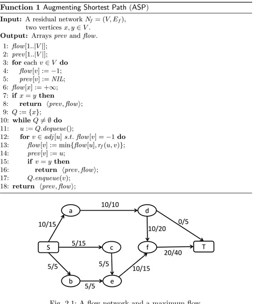
Fig. 2.1: A flow network and a maximum flow.
can be pushed along (a, b)), or no other path from s to a or from b to t can be found.
The following example shows how Algorithm 3 works.
Example 2.1. Consider the flow network and the maximum flow in Figure 2.1. Each edge label x/y states that y is the edge capacity and x is the current flow along the edge. Suppose the edge (c, d) with capacity 15 is added to the network.
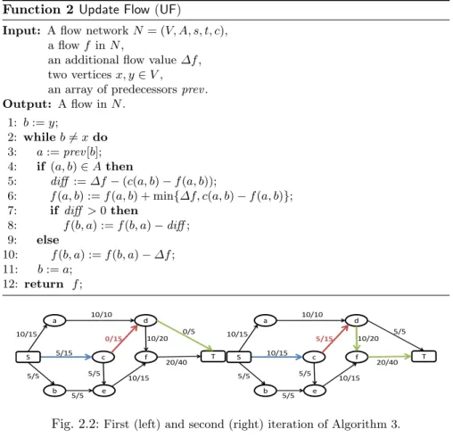
Figure 2.2 shows the augmenting paths computed by Algorithm 3. Specif-ically, Figure 2.2 (left) highlights the path from the source to c (blue-colored
Function 2 Update Flow (UF)
Input: A flow network N = (V, A, s, t, c), a flow f in N ,
an additional flow value ∆f , two vertices x, y ∈ V ,
an array of predecessors prev . Output: A flow in N .
1: b := y;
2: while b 6= x do 3: a := prev [b]; 4: if (a, b) ∈ A then
5: diff := ∆f − (c(a, b) − f (a, b));
6: f (a, b) := f (a, b) + min{∆f, c(a, b) − f (a, b)}; 7: if diff > 0 then 8: f (b, a) := f (b, a) − diff ; 9: else 10: f (b, a) := f (b, a) − ∆f ; 11: b := a; 12: return f ; c 10/20 a 10/15 5/15 5/5 e b 5/5 5/5 10/15 d 10/10 S f T 20/40 0/5 0/15 c 10/20 a 10/15 10/15 5/5 e b 5/5 5/5 10/15 d 10/10 S f T 20/40 5/5 5/15
Fig. 2.2:First (left) and second (right) iteration of Algorithm 3.
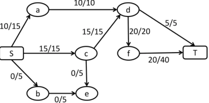
c 15/20 a 10/15 15/15 5/5 e b 5/5 5/5 10/15 d 10/10 S f T 25/40 5/5 10/15
Fig. 2.3: Updated flow network and maximum flow.
edge), whose residual capacity is 10, and the path from d to the sink (green-colored edge), whose residual capacity is 5. The red edge is the new inserted
Algorithm 1 Edge-Insertion-Maintenance (EIM)
Input: A flow network N = (V, A, s, t, c), a maximum flow f in N ,
a pair of vertices (a, b), a capacity w ∈ R+.
Output: A maximum flow for update(N, (a, b), w). 1: if c(a, b) − f (a, b) = 0 then
2: N := update(N, (a, b), w); 3: hprevsa, flowsai := ASP(Nf, s, a); 4: ∆fsa:= flowsa[a];
5: if ∆fsa> 0 then
6: hprevbt, flowbti := ASP(Nf, b, t); 7: ∆fbt:= flowbt[t]; 8: while rf(a, b) > 0 ∧ ∆fsa> 0 ∧ ∆fbt> 0 do 9: ∆f := min{rf(a, b), ∆fsa, ∆fbt}; 10: f (a, b) := f (a, b) + ∆f ; 11: f := UF(N, f, ∆f, s, a, prevsa); 12: f := UF(N, f, ∆f, b, t, prevbt); 13: ∆fsa:= ∆fsa− ∆f ; 14: ∆fbt:= ∆fbt− ∆f ; 15: if rf(a, b) > 0 then 16: if ∆fsa> 0 then
17: hprevbt, flowbti := ASP(Nf, b, t); 18: ∆fbt:= flowbt[t];
19: else if ∆fbt> 0 then
20: hprevsa, flowsai := ASP(Nf, s, a); 21: ∆fsa:= flowsa[a];
22: else
23: hprevsa, flowsai := ASP(Nf, s, a); 24: ∆fsa:= flowsa[a];
25: if ∆fsa> 0 then
26: hprevbt, flowbti := ASP(Nf, b, t); 27: ∆fbt:= flowbt[t];
28: return f ;
one and its residual capacity is 15. The flow across the resulting augmenting path is increased by 5.
Then, as both (c, d) and the path ending in c have still residual capacity after updating the flow, the algorithm looks for a new path in the residual network from d to the sink, and finds the one consisting of the green-colored edges in Figure 2.2 (right). This allows the algorithm to identify a new aug-menting path, the one highlighted in Figure 2.2 (right), along which the flow is increased by 5.
After that, the path from the source to c is saturated, and since there is no other path from the source to c in the residual network, the algorithm
terminates. Figure 2.3 shows the updated network with its new maximum flow.
The following theorems state the correctness and time complexity of Al-gorithm 3.
Theorem 2.2. Given a flow network N , a maximum flow f in N , an edge (a, b), and a capacity w > 0, Algorithm 3 returns a maximum flow in update(N, (a, b), w).
Theorem 2.3. Algorithm 3 runs in O(m min{nm, ∆f }) time, where n = |V |, m = |A|, and ∆f is the maximum flow value’s increase.
In light of the previous theorem, in the presence of small variations of the flow value, our algorithm performs very well, confirming its incremental nature, and, anyway, it never performs worse than the Edmonds-Karp algo-rithm.
2.4.2 Edge Deletions and Capacity Decreases
In this section, we present our algorithm to maintain the maximum flow after decreasing an edge capacity (recall that this case includes also the deletion of an edge). Algorithm 2 below takes as input a flow network N , a maximum flow f in N , an edge (a, b), and a negative capacity w, and computes a maximum flow in update(N, (a, b), w).
The algorithm first computes the amount of flow that (a, b) cannot manage anymore, namely excess (line 1). If excess is positive (i.e., the flow currently assigned to (a, b) exceeds the new capacity), then lines 3–21 are executed. Specifically, the new network is computed (line 3). Then, the flow on (a, b) is set to its new capacity (line 4). After that, the following three phases are performed:
(i) as vertex b has more outgoing than incoming flow, the exceeding one (namely, excess) is sent back from t to b (line 5);
(ii) as vertex a has more incoming than outgoing flow, it tries to push this excess to t along new routes not going through (a, b) (lines 6–13);
(iii) if, after the previous phase, a has still some excess, this is eventually pushed back to s (lines 14–21).
Step (i) above uses the REF function to reduce the flow from a vertex to the sink. Specifically, REF takes as input a flow network N , a flow f in N , a vertex x of N , and a positive real value excess. The function decreases the flow from x to the sink by excess by iteratively searching (in a breadth-first manner) paths from x to the sink having a positive flow on every edge. Example 2.4. Consider the flow network and the maximum flow in Figure 2.3. Suppose we delete the edge (e, f ).
Algorithm 2 Edge Deletion Maintenance (EDM)
Input: A flow network N = (V, A, s, t, c), a maximum flow f in N ,
an edge (a, b) ∈ A, a capacity w ∈ R−.
Output: A maximum flow for update(N, (a, b), w). 1: excess := f (a, b) − max{0, c(a, b) + w};
2: if excess > 0 then
3: N := update(N, (a, b), w); 4: f (a, b) := f (a, b) − excess; 5: f := REF(N, f, b, excess); 6: hprevat, flowati := ASP(Nf, a, t); 7: ∆fat:= min{flowat[t], excess}; 8: while excess > 0 ∧ ∆fat> 0 do 9: excess := excess − ∆fat; 10: f := UF(N, f, ∆f, a, t, prevat); 11: if excess > 0 then
12: hprevat, flowati := ASP(Nf, a, t); 13: ∆fat:= min{flowat[t], excess}; 14: ∆fas:= min{flowat[s], excess}; 15: prevas:= prevat; 16: while excess > 0 do 17: excess := excess − ∆fas; 18: f := UF(N, f, ∆f, a, s, prevas); 19: if excess > 0 then
20: hprevas, flowasi := ASP(Nf, a, s); 21: ∆fas:= min{flowas[s], excess}; 22: return f ;
Figure 2.4 (left) shows the effect of the deletion by highlighting the excess at nodes e and f (red-colored numbers). More specifically, vertex f has a neg-ative excess as it is receiving less flow than that being sent. The REF function sends this flow back to f from the sink, through the only path connecting them—see green-colored edge in Figure 2.4 (right).
Then, the algorithm tries to push the excess at e toward the sink. Fig-ure 2.5 (left) shows the path (blue-colored edges) computed by function ASP: 5 units can be pushed to the sink along this path.
After that, as there is still some excess at e, the algorithm looks for other paths from e to the sink in the residual network, but none is found. As a result, the exceeding flow at e has to be pushed back to the source. Even if the last ASP search did not succeed in finding a path from e to the sink, it found a path from e to the source, which is highlighted in Figure 2.5 (right). The excess at e is decreased along such a path. Figure 2.6 shows the updated network with its new optimal flow.
Function 2 Reset Exceeding Flow (REF)
Input: A flow network N = (V, A, s, t, c), a flow f in N , a vertex x ∈ V , excess ∈ R+. Output: A flow in N . 1: if x 6= t then 2: while excess > 0 do 3: flow [1..|V |]; 4: prev [1..|V |]; 5: for each v ∈ V do 6: flow [v] := −1; 7: prev [v] := NIL; 8: flow [x] := excess; 9: Q := {x}; 10: while Q 6= ∅ do 11: u := Q.dequeue();
12: for v ∈ V s.t. f (u, v) > 0 ∧ flow [v] = −1 do 13: flow [v] := min{flow [u], f (u, v)};
14: prev [v] := u; 15: if v = t then 16: go to line 16; 17: Q.enqueue(v); 18: b := t; 19: while b 6= x do 20: a := prev [b];
21: f (a, b) := f (a, b) − flow [t]; 22: b := a;
23: excess := excess − flow [t]; 24: return f ; c 15/20 a 10/15 15/15 5/5 e b 5/5 5/5 d 10/10 S f T 25/40 5/5 10/15 -10 +10 c 15/20 a 10/15 15/15 5/5 e b 5/5 5/5 d 10/10 S f T 25/40 5/5 10/15 -10 +10
Fig. 2.4: Flow network with excess (left) and paths considered by the REF function (right).
The following theorems state the correctness and the time complexity of Algorithm 2.
c 15/20 a 10/15 15/15 5/5 e b 5/5 5/5 d 10/10 S f T 15/40 5/5 10/15 +10 c 20/20 a 10/15 15/15 5/5 e b 5/5 0/5 d 10/10 S f T 20/40 5/5 15/15 There is sFll some excess on e, thus the algorFhm tries to find another augmenFng path to T, but it can not go further node a (green edges). As a result, the flow has to be pushed back to S. Some flow goes across the previously founded path, stopping to S. +5
Fig. 2.5: Augmenting path from e to the sink (left) and augmenting path from e to the source (right).
c 20/20 a 10/15 15/15 0/5 e b 0/5 0/5 d 10/10 S f T 20/40 5/5 15/15
Fig. 2.6: Updated flow network.
Theorem 2.5. Given a flow network N , a maximum flow f in N , an edge (a, b), and a capacity w < 0, Algorithm 2 returns a maximum flow in update(N, (a, b), w).
Theorem 2.6. Algorithm 2 runs in O(m min{nm, excess}) time, where n = |V | and m = |A|.
It is worth noting that Theorem 2.6 says that our algorithm performs very well in the presence of small variations of the flow value, that is, when excess is small, confirming its incremental nature. Moreover, in any case, the algorithm performs no worse than the Edmonds-Karp algorithm.
2.5 Experimental Evaluation
In this section, we report on an experimental evaluation we performed to compare our approach against state-of-the-art algorithms on different families of datasets.
All experiments were run on an Intel i7 3770K 3.5 GHz, 12 GB of memory, running Linux Mint 17.1.
Datasets. We used a variety of networks taken from the following repos-itories: The Maximum Flow Project Benchmark [2] and Computer Vision
Datasets Execution times (secs)
Family Name # of vertices # of edges HIPR PAR P2R HPF BK E-BK E-IBFS EIM EDM multiview gargoyle-med 8,847,362 44,398,548 46.27 22.17 18.81 10.06 88.54 92.16 8.94 0.72 2.37 camel-med 9,676,802 47,933,324 56.14 33.84 27.88 14.26 17.95 17.33 6.88 0.83 4.56 3D segmentation bone-sx6c100 3,899,396 23,091,149 6.58 1.76 1.79 1.68 3.46 3.54 1.47 0.06 0.19 liver6c100 4,161,604 22,008,003 16.47 7.90 7.81 6.66 7.74 7.69 3.32 0.17 0.85 babyface6c100 5,062,504 29,044,746 27.45 14.77 14.05 16.06 6.38 6.50 3.28 0.76 5.19 bone6c100 7,798,788 45,534,951 13.62 3.33 3.46 3.02 4.07 4.16 2.07 0.10 0.71 adhead6c100(64bit) 12,582,916 74,245,555 35.04 11.91 12.43 16.45 17.76 18.41 7.91 0.76 1.97
surface fitting bunny-med 6,311,088 38,739,041 18.33 10.72 12.27 6.60 1.05 1.08 0.84 0.74 0.78
lazy-brush lbrush-mangagirl 593,032 2,379,695 2.81 1.69 1.38 0.45 0.28 0.28 0.22 0.02 0.70 lbrush-elephant 2,370,064 9,492,348 15.17 9.96 9.59 9.82 1.79 1.89 2.46 0.15 1.67 lbrush-bird 2,372,116 9,505,709 16.31 9.03 9.28 10.81 2.72 2.80 2.42 0.16 5.25 lbrush-doctor 2,373,272 9,522,523 11.98 7.54 6.28 2.52 1.15 1.15 0.91 0.07 0.97 PUNCH punch-us22p 1,674,084 4,718,690 4.76 1.67 1.76 3.41 28.51 29.11 6.09 0.14 24.51 punch-us22u 1,674,084 4,718,690 4.02 1.36 1.61 1.34 4.35 4.42 1.40 0.15 0.16 punch-eu22p 2,020,897 5,715,868 10.88 4.05 3.70 2.52 3.41 3.54 1.41 0.26 2.76 punch-eu22u 2,020,897 5,715,868 8.45 2.80 2.55 1.02 1.20 1.24 0.61 0.190 0.090 bisection cal 1,800,723 4,434,236 8.81 3.68 4.05 1.28 0.51 0.53 0.33 0.34 0.12
Table 2.1: Execution times (secs).
Datasets [1]. We chose these datasets as they have been extensively used in the literature to compare maximum flow algorithms (e.g., they have been used in [31, 24]). In particular, we chose the largest networks of different fam-ilies. Details are reported in (the first four columns of) Table 2.1. Most of the networks have millions of vertices (up to 12.5M vertices) and tens of millions of edges (up to 74M edges).
Algorithms. We compared our algorithms against state-of-the-art al-gorithms for the maximum flow computation, namely HIPR [13], PAR [29], P2R [30], HPF [41], BK [8], E-BK [48], and E-IBFS [31] (see Section 3.2 for a discussion of them). We used the implementations of the algorithms provided by their authors. Our algorithms were written in Java.
Results. For each of the datasets listed in Table 2.1, we randomly chose 250 edges to be inserted and 250 edges to be deleted. The EIM (resp. EDM) column reports the average time taken by our insertion (deletion) algorithm to handle the 250 edge insertions (deletions). The average time taken by each of the competitors to handle the edge insertions slightly differs from the average time taken to handle the edge deletions (the difference was on the order of 10−2 seconds or less), so we report only one time. Thus, each competitor’s running time in Table 2.1 is to be interpreted as both the average time to handle the 250 insertions and the average time to handle the 250 deletions. The reason of the negligible difference between the two average times is that a one-edge modification does not affect much the overall running time, which is mainly determined by the size of the whole network.
To ease readability, for each dataset, the lowest running times are high-lighted in blue. As for edge insertions, EIM is always the fastest algorithm,
except for the last dataset, where E-IBFS is faster, even though the difference is negligible. In most of the cases (around 75% of the datasets), EIM is more efficient than the second-fastest algorithm by at least one order of magnitude. Regarding deletions, EDM is the fastest algorithm in most of the cases. In the remaining cases E-IBFS is the fastest one, with the only exception of the punch-us22p dataset. However, we point out that E-IBFS computes only the value of a flow, rather than the flow function, while EDM computes the flow function (which gives the flow for each edge). For the punch-us22p dataset, the fastest algorithm is PAR (which is based on the push-relabel approach), while algorithms based on augmenting paths showed poor performances in this case.
Finally, we observe that handling edge deletions showed to be more ex-pensive than handling edge insertions.
2.6 Discussion
While many algorithms have been proposed for the maximum flow problem, many current applications deal with dynamic networks and thus call for in-cremental algorithms, as it is impractical to compute the new maximum flow from scratch every time updates occur.
We have proposed efficient incremental algorithms to maintain the max-imum flow in evolving networks. Experimental results have shown that our approach outperforms state-of-the-art algorithms and can easily handle net-works with millions of vertices and tens of millions of edges.
We point out that our algorithms can be directly applied to incrementally maintain the minimum cut too, because of the well-known max-flow/min-cut theorem (i.e., the maximum flow value is equal to the minimum cut capacity), thereby widening further the range of applications.
As directions for future work, we plan to generalize our algorithms to handle batches of updates at once, and leverage graph database systems.
Incremental Maintenance of All-Pairs Shortest
Paths in Relational DBMSs
Computing shortest paths is a classical graph theory problem and a central task in many applications. Although many algorithms to solve this problem have been proposed over the years, they are designed to work in the main memory and/or with static graphs, which limits their applicability to many current applications where graphs are highly dynamic, that is, subject to frequent updates.
In this chapter, we present novel efficient incremental algorithms for main-taining all-pairs shortest paths and distances in dynamic graphs [35, 37]. We experimentally evaluate our approach on several real-world datasets, show-ing that it significantly outperforms current algorithms designed for the same problem.
3.1 Introduction
Computing shortest path and distances has a wide range of applications in social network analysis [46], road networks [63], graph pattern matching [22], biological networks [55], and many others. It is both an important task in its own right (e.g., if we want to know how close people are in a social network) and a fundamental subroutine for many advanced tasks.
For instance, in social network analysis, many significant network metrics (e.g., eccentricity, diameter, radius, and girth) and centrality measures (e.g., closeness and betweenness centrality) require knowing the shortest paths or distances for all pairs of vertices. There are many other domains where it is needed to compute the shortest paths (or distances) for all pairs of ver-tices, including bioinformatics [52] (where all-pairs shortest distances are used to analyze protein-protein interactions), planning and scheduling [51] (where finding the shortest paths for all pairs of vertices is a central task to solve binary linear constraints on events), and wireless sensor networks [15] (where different topology control algorithms need to compute the shortest paths or distances for all pairs of vertices).
Though several techniques have been proposed to efficiently compute shortest paths/distances, they are designed to work in the main memory and/or with static graphs. This severely limits their applicability to many current applications where graph are dynamic and the graph along with the shortest paths/distances do not fit in the main memory. When graphs are subject to frequent updates, it is impractical to recompute shortest paths or distances from scratch every time a modification occurs.
To overcome these limitations, we propose efficient algorithms for the in-cremental maintenance of all-pairs shortest paths and distances in dynamic graphs stored in relational DBMSs.
Contributions. We consider the setting where graphs and shortest paths are stored in relational DBMSs and propose novel algorithms to incrementally maintain all-pairs shortest paths and distances after vertex/edge insertions, deletions, and updates. The proposed approach aims at reducing the time needed to update the shortest paths by identifying only those that need to be updated (it is often the case that small changes affect only few shortest paths).
To the best of our knowledge, [50] is the only disk-based approach in the literature for incrementally maintaining all-pairs shortest distances. In partic-ular, like our approach, [50] relies on relational DBMSs. We experimentally compare our algorithms against [50] on five real-world datasets, showing that our approach is significantly faster. It is worth noticing that our approach is more general than [50] in that we keep track of both shortest paths and distances, while [50] maintain shortest distances only (thus, there is no infor-mation on the actual paths).
3.2 Related Work
Different variants of the shortest path problem have been investigated over the years: single-pair shortest path (SPSP)—find a shortest path from a given source vertex to a given destination vertex; single-source shortest paths (SSSP)—find a shortest path from a given source vertex to each vertex of the graph; all-pairs shortest paths (APSP)—find a shortest path from x to y for every pair of vertices x and y.
Variants of these problems where we are interested only in the shortest distances, rather than the actual paths, have been studied as well. We will use SPSD, SSSD, and APSD to refer to the single-pair shortest distance, single-source shortest distances, and all-pairs shortest distances problems, re-spectively.
In this section, we discuss the approaches in the literature to solve the above problems. We first consider non-incremental algorithms, and then in-cremental ones.
Non-Incremental Algorithms. Since the introduction of the Dijkstra’s al-gorithm [19], a plethora of alal-gorithms have been proposed to improve on its performance (see [59] for a recent survey).
Most of the recently proposed methods require a preprocessing step for building index structures to support the fast computation of shortest paths and distances [11, 44, 4, 34, 65, 53, 54, 66, 12, 27].
Specifically, [11, 44, 4] address the SPSD problem, and a similar approach for the SPSP problem has been proposed in [34]. [65] considers both the SPSP and SPSD problems. There have been also proposals addressing the approximate computation of SPSD [53, 54]. These methods are based on the selection of a subset of vertices as “landmarks” and the offline computation of distances from each vertex to those landmarks. [66] and [12] propose based index structures for solving the SSSP and SSSD problems, while disk-based index structure for the SPSP and SPSD problems have been proposed in [27].
[28] addresses the SPSP problem and, like our approach, relies on relational DBMSs.
Besides the fact that most of the aforementioned techniques assume that graphs, shortest paths/distances, and auxiliary index structures fit in the main memory (which is not realistic in many current applications), the main limit of all the approaches mentioned above is that they need to recompute a so-lution from scratch every time the graph is modified, even if we make small changes affecting a few shortest paths/distances. In many cases this requires an expensive pre-processing phase to build the index structures that are nec-essary to answer queries. Then, of course, shortest paths/distances have to be computed again for all pairs. Thus, these methods work well if the graph is static. In contrast, if the graph is dynamic, the expensive pre-processing phase and the re-computation of all shortest paths/distances have to be done every time a change is made to the graph, and this is impractical for large graphs subject to frequent changes.
Incremental Algorithms. Several approaches have been proposed to incre-mentally maintain shortest paths and distances when the graph is modified. [43] introduces data structures to support APSP maintenance after edge tions in directed acyclic graphs. [17] considers both edge insertions and dele-tions. [5] presents a hierarchical scheme for efficiently maintaining all-pairs approximate shortest paths in undirected unweighted graphs and in the pres-ence of edge deletions. [47] proposes an algorithm for maintaining all-pairs shortest paths in directed graphs with positive integer weights bounded by a constant. Another approach for the incremental maintenance of APSPs is [46]. [14] proposes an algorithm for maintaining nearest neighbor lists in weighted
graphs under vertex insertions and decreasing edge weights. The approach is tailored for scenarios where queries are much more frequent than updates.
Approximate APSP maintenance in unweighted undirected graphs has been addressed in [5, 57, 40], while [6] considered edge deletions and weight increases in weighted directed graphs.
All the techniques above share the use of specific complex data struc-tures and work in the main memory, which limits their applicability. In fact, as pointed out in [16, 18], memory usage is an important issue of current approaches, limiting substantially the graph size that they can handle (for instance, the experimental studies in [16, 18] could not go beyond graphs of 10,000 vertices).
Algorithms to incrementally maintain APSDs for graphs stored in rela-tional DBMSs have been proposed in [50]. These algorithms improve on [39] (which addresses the more general view maintenance problem in relational databases) by avoiding unnecessary joins and tuple deletions. However, [50] can deal only with the APSD maintenance problem while [39] works with general views (both in SQL and Datalog).
To the best of our knowledge, [50] is the only disk-based approach for maintaining APSDs (incremental algorithms to find a path between two ver-tices in disk-resident route collections have been proposed in [7], but paths are not required to be shortest ones). We are not aware of disk-based approaches to incrementally maintain APSPs. [50] is the closest work to ours, but with significant differences.
First, our algorithms maintain both shortest paths and shortest distances, while [50] is able to maintain shortest distances only—knowing the actual (shortest) paths is necessary in different applications.
Second, while both [50] and our algorithms proceed by first identifying “af-fected” shortest paths (i.e., those whose distance might need to be updated after the graph is changed) and then acting on them, the two approaches differ in how this is done. Specifically, the strategy employed by our approach to identify affected shortest paths is different and more effective. For both edge insertions and deletions, we have two distinct phases, one looking forward and the other looking backward. This allows us to filter out earlier shortest paths that do not play a role in the maintenance process. On the other hand, [50] identifies affected shortest paths in a more blind way: for both edge in-sertions and deletions, all shortest distances starting at the inserted/deleted edge are combined with all shortest distances ending in the inserted/deleted edge, leading to computationally expensive joins. Moreover, in our deletion algorithm, the recomputation of deleted shortest distances is done in an in-cremental way, as opposed to [50], which performs this step by combining all shortest distances that are left after the deletion phase.
Third, as shown in our experimental evaluation (cf. Section 3.5), our al-gorithms are significantly faster than those of [50].
The algorithms proposed in this chapter generalize the ones presented in [35] in that the former are able to maintain both shortest paths and dis-tances, while the latter maintain shortest distances only.
3.3 Preliminaries
In this section, we introduce the notation and terminology used in the rest of this chapter.
A graph is a pair (V, A), where V is a finite set of vertices and A ⊆ V × V is a finite set of pairs called edges. A graph is undirected if A is a set of unordered pairs; otherwise (edges are ordered pairs) it is directed. A (directed or undirected) weighted graph consists of a graph G = (V, A) and a function ϕ : A → R+ assigning a weight (or distance) to each edge in A.1 We use ϕ(u, v) to denote the weight assigned to edge (u, v) by ϕ.
A sequence v0, v1, . . . , vn (n > 0) of vertices of G is a path from v0 to vn
iff (vi, vi+1) ∈ A for every 0 ≤ i ≤ n − 1. The weight (or distance) of a path
p = v0, v1, . . . , vn is defined as ϕ(p) =P n−1
i=0 ϕ(vi, vi+1). Obviously, there can
be multiple paths from v0 to vn, each having a distance. A path from v0 to
vn with the lowest distance (over the distances of all paths from v0 to vn) is
called a shortest path from v0to vn(there can be multiple shortest paths from
v0 to vn) and its distance is called the shortest distance from v0 to vn. We
assume that the shortest distance from a vertex to itself is 0, and the shortest distance from a vertex v0 to a distinct vertex vn is not defined if there is no
path from v0to vn.
In the rest of the chapter we consider directed weighted graphs and call them simply graphs—the extension of the proposed algorithms to undirected graphs is trivial. Without loss of generality, we assume that graphs do not have self-loops, i.e., edges of the form (v, v) (the reason is that self-loops can be disregarded for the purpose of finding shortest distances).
We consider the case where graphs and shortest paths are stored in rela-tional databases. Notice that this allows us to take advantage of full-fledged optimization techniques provided by relational DBMSs.
Specifically, the set of edges of a graph is stored in a ternary relation E containing a tuple (a, b, w) iff there is an edge in the graph from a to b with weight w. We call E an edge relation. Vertices without incident edges can be ignored for our purposes.
A relation SP of arity 4 is used to represent the shortest paths for all pairs of reachable vertices of the graph (obviously, for a pair of reachable vertices we keep track of only one shortest path). Specifically, a shortest path v0, v1, . . . , vn(n ≥ 1) from v0to vnwith (shortest) distance d0n is represented
with the set of tuples {(v0, vi, d0i, vi−1) | 1 ≤ i ≤ n} in SP , where d0idenotes
the shortest distance from v0 to vi. Clearly, it is always possible to build 1