D
IPARTIMENTO DI
F
ISICA
D
OTTORATO DI
R
ICERCA IN
S
CIENZE E
T
ECNOLOGIE
F
ISICHE
, C
HIMICHE E DEI
M
ATERIALI
C
ICLO
XXXI
M
EASUREMENTS OF TOP QUARK PAIR
PRODUCTION DIFFERENTIAL CROSS SECTIONS IN
√
THE
A
LL
-H
AD
RONIC DECAY CHANNEL IN
pp
COLLISIONS AT
s
=13 T
E
V
USING THE
ATLAS
DETECTOR
S
ETTORE
S
CIENTIFICO DISCIPLINARE
FIS/01
C
OORDINATORE:
PROF. VINCENZO CARBONES
UPERVISORE:
PROF. ENRICO TASSIAbstract
In this thesis, the measurements of the differential cross sections of top quark pair production in proton - proton collisions at a center of mass energy of √
s = 13 TeV are presented. Data are collected at the LHC by the ATLAS
detector during the 2015 and 2016 data-taking periods, corresponding to an
integrated luminosity of L = 36.1 fb−1. The top quark pair events are
se-lected in the fully hadronic decay channel, resolved regime. The measure-ments are presented for several kinematics spectra and for observables sen-sitive to Initial and Final State Radiation. The measured spectra are corrected for detector effects and are compared to several theoretical Monte Carlo sim-ulations. The measured spectra provide stringent tests of perturbative QCD, gives a better understanding of the top quark pair production mechanism and can be used to tune the Monte Carlo simulations. In addition, the ex-pected performance of the Inner Tracker and the High Granularity Timing Detector, which will be installed during the Phase II upgrade of the ATLAS detector, will be presented.
Abstract
In questa tesi verrà presentata la misura delle sezioni d’urto differenziali di produzione di coppie di quark top-antitop in collisioni protone - protone ad
un’energia nel centro di massa di √s = 13 TeV. I dati sono stati raccolti
ad LHC dal detector ATLAS durante il 2015 e il 2016 e corrispondono ad
una luminosità integrata diL = 36.1 fb−1. I candidati eventi t¯t sono stati
selezionati nel canale di decadimento completamente adronico, in regime risolto. La misura viene presentata in funzione di diverse osservabili; sia
relative alla cinematica del sistema t¯tche osservabii particolarmente sensibili
all’emissione di gluoni da parte dei quark top nello stato iniziale e finale. Gli spettri misurati sono poi corretti per tenere conto degli effetti indotti dal de-tector e sono poi confrontati con diverse predizioni Monte Carlo. Tali misure consentono di effettuare dei test stringenti della QCD perturbativa, garantis-cono una migliore comprensione dei meccanismi di produzione delle coppie di quark top-antitop e possono essere usati per la calibrazione dei parametri caratteristici delle simulazioni Monte Carlo. Inoltre, verranno presentate le performance attese dell’Inner Tracker e dell’High Granularity Timing Detec-tor, i quali saranno installati durante l’upgrade di Fase II del rilevatore AT-LAS.
Contents
Abstract i
Introduction xxxvi
1 Theory foundations 1
1.1 The Standard Model of Particle Interactions . . . 1
1.2 Quantum Electrodynamics. . . 3
1.3 Quantum Chromodynamics . . . 4
1.4 Weak Interactions . . . 7
1.5 Electroweak theory . . . 7
1.6 Spontaneous symmetry breaking mechanism . . . 9
1.7 Principles of collider physics . . . 11
1.7.1 Factorization Theorem . . . 11
1.7.2 Parton Density Functions . . . 12
1.7.3 Luminosity at proton-proton colliders . . . 14
1.8 The top quark at the LHC . . . 15
1.8.1 Top quark properties . . . 15
1.8.2 Top quark decay modes . . . 18
1.8.3 Top quark pair production. . . 20
1.8.4 Charge asymmetry in t¯tquark pair production . . . 23
1.8.5 Single top quark production. . . 23
2 The ATLAS Detector at the LHC 25 2.1 The Large Hadron Collider . . . 25
2.1.1 The LHC experiments . . . 29
2.1.2 The Worldwide LHC Computing Grid. . . 30
2.2 The ATLAS Detector . . . 32
2.2.1 Coordinate system . . . 34
2.2.2 Magnet system . . . 35
2.2.3 Inner Detector . . . 36
Silicon pixel tracker and the Insertable B-Layer (IBL) . 38 SemiConductor Tracker (SCT). . . 38
Transition Radiation Tracker (TRT) . . . 38
2.2.4 Calorimetry . . . 38
Electromagnetic calorimetry. . . 40
Hadronic calorimeter. . . 40
Forwards calorimeter . . . 41
2.2.5 Muon Spectrometer . . . 41
Catode Strip Chambers . . . 42
Resistive Plate Chambers . . . 43
Thin Gap Chambers . . . 43
2.2.6 Forward detectors . . . 43
2.2.7 Trigger and data acquisition . . . 44
Level 1 trigger . . . 45
The High Level Trigger . . . 45
Data Acquisition . . . 45
2.2.8 Trigger strategy in the cross section measurement . . . 46
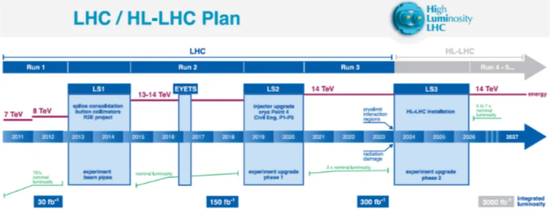
3 The ATLAS Detector at the HL-LHC 50 3.1 From the LHC to the HL-LHC . . . 50
3.2 The Inner Tracker . . . 53
3.2.1 The ITk layout . . . 54
3.2.2 Tracking and physics performance . . . 55
Tracking and vertexing performance . . . 55
Physics object performance . . . 59
3.3 The High Granularity Timing Detector . . . 62
3.3.1 HGTD layout . . . 63
3.3.2 Performance studies . . . 63
Track extrapolation to the HGTD . . . 64
Track-to-vertex association . . . 65
Jet performance . . . 66
4 Event reconstruction at the ATLAS experiment 68 4.1 Monte Carlo event generation . . . 68
4.1.1 Hard processes . . . 70 4.1.2 Parton showers . . . 71 4.1.3 Hadronization. . . 74 String model. . . 76 Cluster model . . . 77 4.1.4 Hadron decays . . . 78 4.1.5 Underlying event . . . 78 4.1.6 Generator filtering . . . 79
4.2 ATLAS detector simulation . . . 80
4.2.1 ATLAS simulation overview . . . 80
4.2.2 Simulated ATLAS detector geometry . . . 81
4.2.3 Digitalization . . . 82
4.2.4 Fast simulations . . . 82
4.3 Object reconstruction . . . 84
4.4 Samples adopted for the cross section measurement . . . 85
4.4.1 Data samples . . . 85
4.4.2 Monte Carlo samples . . . 85
5 Object reconstruction performance of the ATLAS detector 88 5.1 Tracking performance . . . 88
5.1.1 Track reconstruction . . . 89
5.2 Vertexing performance . . . 94
5.2.1 Primary vertex reconstruction. . . 94
5.2.2 Vertices truth classification . . . 95
5.2.3 Vertex performance. . . 97
5.3 Photon performance . . . 99
5.3.1 Photon reconstruction . . . 99
5.3.2 Photon identification . . . 100
5.3.3 Photon isolation. . . 101
5.3.4 Photon identification efficiency . . . 102
5.4 Electron performance . . . 105 5.4.1 Electron reconstruction . . . 105 5.4.2 Electron identification . . . 106 5.4.3 Electron isolation . . . 106 5.4.4 Electron efficiency . . . 107 5.5 Muon performance . . . 108 5.5.1 Muon reconstruction . . . 108 5.5.2 Muon identification . . . 109 5.5.3 Muon isolation . . . 110 5.5.4 Muon efficiency . . . 111 5.6 Tau performance . . . 112 5.6.1 Tau reconstruction . . . 112 5.6.2 Tau identification . . . 113
5.6.3 Tau identification efficiency . . . 113
5.7 Jet performance . . . 114
5.7.1 Jet reconstruction . . . 115
5.7.2 Jet energy scale calibration . . . 115
5.7.3 Pile up corrections . . . 116
5.7.4 Jet energy scale and η calibration . . . 117
5.7.5 Global sequential calibration . . . 117
5.7.6 In situ calibration . . . 118
5.7.7 Systematic uncertainties . . . 118
5.8 B-tagged jet performance. . . 120
5.8.1 MV2c10 b-tagging algorithm . . . 120
5.8.2 Calibration methods . . . 121
T&P method . . . 122
LH method . . . 123
5.8.3 b-jet tagging efficiencies . . . 123
5.9 ETmissperformance . . . 125
5.9.1 Emiss T reconstruction . . . 126
Emiss T hard term . . . 126
ETmiss soft term . . . 129
5.9.2 Systematic uncertainties . . . 130
5.9.3 Emiss T resolution . . . 131
6 Analysis strategy and techniques 135 6.1 The fully hadronic t¯tdecay channel in the resolved topology . 135 6.2 Measured observables . . . 137
6.2.1 t¯tsystem kinematics . . . 137
6.2.2 ISFR-sensitive t¯tsystem spectra. . . 137
6.3 Objects definitions . . . 139 6.3.1 Jets . . . 139 6.3.2 Electrons . . . 140 6.3.3 Muons . . . 140 6.3.4 τ jets . . . 140 6.3.5 B-Tagging . . . 141 6.3.6 Overlap removal . . . 141 6.3.7 Event cleaning . . . 142
Good Run List. . . 142
Corrupted data . . . 142
Vertex Requirement . . . 142
6.3.8 Particle level objects definition . . . 142
6.3.9 Parton level objects definition . . . 143
6.4 Topology-based event preselection . . . 143
6.5 t¯tsystem reconstruction . . . 144
6.6 Event selection. . . 146
6.7 Background determination. . . 148
6.7.1 Monte Carlo-based background estimation . . . 149
6.7.2 Data-driven multi-jet QCD background estimation . . 150
6.8 Reconstructed level results . . . 153
7 Unfolding strategy 162 7.1 The unfolding problem . . . 162
7.2 The iterative D’Agostini unfolding technique . . . 163
7.3 Unfolding procedure . . . 165
7.4 Unfolding validation . . . 168
7.4.1 Closure tests . . . 168
7.4.2 Stress tests . . . 168
7.4.3 Test on the number of iterations . . . 170
8 Systematic uncertainties 172 8.1 Detector uncertainties . . . 172 8.1.1 Jet reconstruction . . . 173 8.1.2 b-tagging . . . 173 8.1.3 Lepton reconstruction . . . 173 8.1.4 τ reconstruction . . . 174 8.1.5 ETmiss reconstruction . . . 174 8.2 Modelling uncertainties . . . 174
8.2.1 Matrix element and parton shower models . . . 174
8.2.2 Initial and Final State Radiation . . . 175
8.2.3 PDF. . . 175
8.2.4 MC sample finite statistics . . . 176
8.3 Background uncertainties . . . 176
8.3.1 t¯tnormalization . . . 176
8.3.2 Data-driven multi-jet estimation . . . 176
8.5 Uncertainties affecting the measurement. . . 177
8.5.1 Systematics breakdown, particle level . . . 177
8.5.2 Systematics breakdown, parton level . . . 188
9 Results 192 9.1 Unfolded distributions . . . 192
9.1.1 Particle level unfolded distributions . . . 192
9.1.2 Parton level unfolded distributions . . . 203
9.2 χ2evaluation. . . 203
Conclusions 210 A Stability of the t¯treconstruction method 212 B Implementation of the χ2 minimization algorithm 217 C Cutflows for data and MC-estimated processes 226 D Systematic uncertainties breakdown tables 232 D.1 Absolute cross sections, unfolded to particle level . . . 232
D.2 Relative cross sections, unfolded to particle level . . . 252
D.3 Absolute cross sections, unfolded to parton level . . . 252
D.4 Relative cross sections, unfolded to parton level . . . 260
E Unfolding corrections 268 E.1 Corrections at particle level . . . 268
E.2 Corrections at parton level . . . 288
F Unfolding stability tests 294 F.1 Closure tests . . . 294
F.1.1 Closure, particle level . . . 294
F.1.2 Closure, parton level . . . 300
F.2 Stress tests . . . 301
F.2.1 Stress test, particle level . . . 301
F.2.2 Stress test, parton level . . . 321
F.3 Unfolding iterations stability checks . . . 329
G Covariance matrices 339
List of Figures
1.1 Properties of fundamental particles in the SM framework. Val-ues are taken from [9] . . . 3
1.2 Comparison of the values of αs(Q) obtained from fits to the
TEEC [15] functions (red star points) with the uncertainty band from the global fit (orange full band) and the 2016 world av-erage (green hatched band). Determinations from other mea-surements from D/0 and CMS experiments are also shown. The error bars include all experimental and theoretical sources of uncertainty. . . 6
1.3 The Higgs potential µ2Φ†Φ − λ[Φ†Φ]2 for λ > 0. In case (a), no
degeneration of the ground state occurs; in case (b), a degener-ate circle of minimum potential exists and an arbitrary choice for the ground state can be made. . . 10
1.4 Schematic representation of the Factorization Theorem for hadron-hadron cross section. . . 11
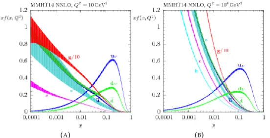
1.5 NNLO PDFs from the MMHT14 set evaluated at Q2 = 10GeV (a)
and Q2 = 104 GeV (b). The associated solid bands represent
the 68% confidence-level uncertainties. The Figures has been taken from [28] . . . 13
1.6 Summary of the ATLAS and CMS direct mt measurements.
The results are compared with the LHC and Tevatron+LHC mtcombinations. For each measurement, the statistical
uncer-tainty and the sum in quadrature of the statistical and system-atic uncertainties are shown. The results below the solid black line have been produced after the LHC and Tevatron+LHC combinations were performed. Figure taken from [41]. . . 16
1.7 Summary of measured W helicity fractions by ATLAS and CMS at 7 and 8 TeV, compared to the respective theory predictions. The uncertainty on the theory predictions is shown by a green band, the total experimental uncetainties are given by the sum in quadrature of the statisical and systematic ones. Figure taken from [41] . . . 18
1.8 Pie charts showing the Branching Ratios of the single top quark (a) and top-antitop quark pair production (b). Data is taken from [9]. 19
1.9 Feynman diagrams for the single top quark decay modes (a), t¯tcompletely hadronic (b), semileptonic (c) and dileptonic (d). 19
1.10 Feynman diagrams for the top-antitop quark pair production at Leding Order of perturbation expansion: gluon-gluon fu-sion (a) in the t (left), u (center) and s (right) channels and quark-antiquark annihilation (b). . . 20
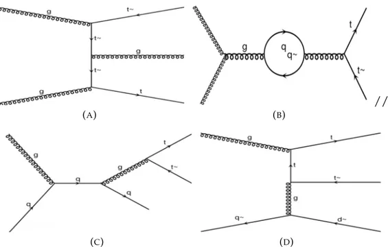
1.11 Selection of feynman diagrams for the top-antitop quark pair production at NLO of perturbation expansion: real quark emis-sion (a), virtual loop correction (b), qg interaction (c) and ¯qg interaction (d). . . 21
1.12 Summary of LHC and Tevatron measurements of the top-pair production cross section as a function of the center of mass en-ergy compared to the NNLO+NNLL QCD calculations at mt=
172.5 GeV. The theory band represents uncertainties due to renormalisation and factorisation scale, parton density func-tions and the strong coupling. Figure taken from [41]. . . 22
1.13 Summary of the charge asymmetry measurements on ATLAS and CMS at 8 TeV showing both the inclusive measurements and the measurement using boosted events, compared to the respective theory predictions. Figure taken from [41]. . . 22
1.14 Feynman diagrams for the single top quark production at LO of perturbation expansion: association production with a real W (a), t-channel (b) and s-channel (c). . . 24
1.15 Summary of ATLAS and CMS measurements of the single top quark production cross sections in various channels as a func-tion of the center of mass energy. The measurements are com-pared to theoretical calculations based on: NLO QCD, NLO QCD complemented with NNLL resummation and NNLO QCD (t-channel only). Figure taken from [41] . . . 24
2.1 Bird’s-eye view of the LHC accelerator complex and its exper-iments. . . 25
2.2 Cumulative luminosity versus time delivered to (green) and recorded by ATLAS (yellow) during stable beams for pp colli-sions at 7 TeV center of mass energy in 2010 (a) and 2011 (b), at 8 TeV center of mass energy in 2012 (c) and at√s = 13TeV in 2015 (d), 2016 (e), 2017 (f) and 2018 (g). The delivered lu-minosity accounts for lulu-minosity delivered from the start of stable beams until the LHC requests ATLAS to put the detec-tor in a safe standby mode to allow for a beam dump or beam studies. Figures taken from [53,54]. . . 27
2.3 Scheme of a cryodipole superconducting magnet at the LHC. Figure taken from [8]. . . 28
2.4 Scheme of a four-cavity cryomodule at the LHC. Figure taken from [8]. . . 28
2.5 The CERN accelerator complex. The four yellow dots along the LHC rings correspond to the four interacting points where the major experiments are collocated. Figure taken from [55].. 29
2.6 Schematic representation of the WLCG tiers. Dedicated “dark-fiber” connections between CERN and each of the Tier 1 sites were implemented to ensure the necessary data rates. These connections are supplemented with secondary connections to ensure reliability of the network. Connectivity between Tier 1 and Tier 2 sites is provided by national and international academic and research network infrastructures. Figure taken from [65]. . . 31
2.7 Schematic overview of the ATLAS detector and its subdetec-tors. Figure taken from [66]. . . 34
2.8 Illustration of the ATLAS Detector oriented in the global coor-dinate system. Figure taken from [67]. . . 35
2.9 Layout of the ATLAS magnet system. Figure extracted and adapted from [68].. . . 36
2.10 Cut-away view of the ATLAS ID during Run 1. The IBL is not shown since it has been installed during Run 2. Figure taken from [57]. . . 37
2.11 Sketch of the ATLAS inner detector showing all its compo-nents, including the new insertable B-layer (IBL). The distances to the interaction point are also shown. Figure taken from [69]. 37
2.12 Cut-away view of the ATLAS calorimeter system. Figure taken from [57]. . . 39
2.13 Photograph of a partly stacked barrel electromagnetic LAr mod-ule. The acccordion structure is clearly visible. Photograph taken from [57]. . . 40
2.14 Cut-away view of the ATLAS muon spectrometer. Figure taken from [57]. . . 41
2.15 Schematic view of the forward ATLAS detectors. Their place-ment along the beam-line around the ATLAS IP in also shown. Figure taken from [57]. . . 43
2.16 Diagram of the ATLAS Trigger and Data Acquisition system in Run 2 showing expected peak rates and bandwidths through each component. Figure taken from [71]. . . 44
2.17 Trigger efficiency curves as a function of the 6th jet transverse
mo-mentum, for different values of the maximum allowed η of the jets. In particular, the ηcut values are 2.0 (a), 2.1 (b), 2.2 (c), 2.3 (d) and
2.4 (e). These are computed in data and for a ttbar MC sample,
se-lecting events with two b-tagged jets. . . 48
2.18 Trigger efficiency curves as a function of the 6th jet transverse
mo-mentum, for different values of the maximum allowed η of the jets. In particular, the ηcut values are 2.0 (a), 2.1 (b), 2.2 (c), 2.3 (d) and
2.4 (e). These are computed in data and for a ttbar MC sample,
se-lecting events with zero b-tagged jets. . . 49
3.2 (a): Schematic representation of the ITk Inclined Duals layout. Only one quadrant and only active detector elements are shown. The active elements of the barrel and end-cap Strip Detector are shown in blue, for the Pixel Detector the sensors are shown in red for the barrel layers and in dark red for the end-cap rings. The horizontal axis is along the beam line with zero being the interaction point. (b): Cut-away view of the ITk In-clined Layout Geant4 [86] geometry model. The Figures have been taken from [80]. . . 54
3.3 Radiation lenght X0versus η for the current ID (a) and Inclined
Duals ITk (b), . Only positive η are shown due to detector sym-metry. The Figures have been taken from [80]. . . 55
3.4 (a): Track reconstruction efficiency for a top-pair sample with an average of 200 pile up events. Overlaid are the results for the current Run 2 detector. (b): Fake rate for reconstructed tracks in t¯t events with < µ >= 200 using the truth particle matching criterion Pmatch. ITk is compared to the Run 2
de-tector results for two different levels of track selection. The Figures have been taken from [80]. . . 56
3.5 Track parameter resolution in d0 (a), z0(b) and pT (c) as a
func-tion of η for the Inclined Duals ITk layout. Results are shown for single muons with pT of 1, 10 and 100 GeV. Performance
results from Run 2 ID are shown for comparison. The Figures have been taken from [80]. . . 57
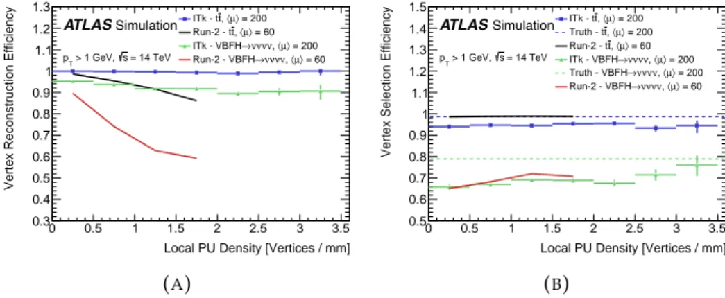
3.6 The primary vertex reconstruction (a) and identification (b) ef-ficiency for t¯tand vector boson fusion H → νννν interactions as a function of local pile up density in events with an average pile up of 200. The vertex identification is done using the Σp2
T
criterion. The dotted lines on the right plot indicate the rate of events for the ITk where the true primary interaction vertex actually has the highest true Σp2
T. Shown as well are results
for a Run 2 simulation sample using the Run 2 primary vertex reconstruction code. The Figures have been taken from [80]. . 58
3.7 z0 resolution as a function of η for different pT values. Figure
taken from [83]. . . 59
3.8 The rejection of pile up jets as a function of the efficiency for hard-scatter jets with 20 < pT < 40GeV (a) and pT > 40GeV (b)
using the RpT discriminant in di-jet events with an average of
200 pile up events. The Figures have been taken from [80]. . . 60
3.9 The resolutions of Emiss
T in Monte Carlo t¯t events with an
av-erage of 200 pile up events. The resolutions are shown as a function of the local pile up vertex density around the hard-scatter vertex, for three different ETmiss definitions. The first (blue) considers only tracks in the region |η| < 2.5 for both pile up jet rejection and ETmiss soft term. The second (red) uses hard tracks up |η| of 4. The third (black) uses tracks up to |η| < 4.0. Figure taken from [80]. . . 62
3.10 Exploded view of the various components of the HGTD, ex-cluding the cooling plates. Figure taken from [83]. . . 63
3.11 Efficiencies for matching tracks to at least one pixel in the HGTD in single pion events (a) and for correctly reconstructing the time of a track in simulated VBF events with < µ >= 200 (b). An exponential fit is performed on the points and the parame-ters of the fit are shown. The Figures have been taken from [83]. 64
3.12 (a): View in the Rz plane of the tracks associated to the pri-mary vertices in a simulated VBF event at < µ >= 200. The distribution of tracks associated to the hard-scatter vertex as a function of reconstructed times and z position is shown in (b). For convenience, the projections on z and t are presented in (c) and (d), respectively. The Figures have been taken from [83]. . 65
3.13 Pile up jet rejection as a function of hard-scatter jet efficiency in the 2.4 < |η| < 4.0 region for jets with 30 < pT < 50GeV (a)
and pT > 50 GeV (b) and hard-scatter jet efficiency versus
|η| for a 2% pile up jet efficiency rejection for jets with 30 < pT < 50 GeV (c) and pT > 50 GeV (d). The curves refer to the
ITk-only and ITk + HGTD scenarios with different time res-olutions. The results have been obtained for di-jet simulated Monte Carlo events. The Figures have been taken from [83]. . 67
4.1 Schematic representation of a hadron-hadron collision as sim-ulated by a MC event generator. The red blob in the center rep-resents the hard collision, surrounded by a tree-like structure representing Bremsstrahlung as simulated by parton show-ers. The purple blob indicates a secondary hard scattering event. Parton-to-hadron transitions are represented by light green blobs, dark green blobs indicate hadron decays, while yellow lines signal soft photon radiation. Figure taken from [93]. 69
4.2 Schematic representation of parton shower. Figure extracted from Figure 4.1. . . 72
4.3 Schematic representation of parton shower in the dipole ap-proach. Figure taken from [94]. . . 73
4.4 Schematic representation of string (a) and cluster (b) hadroniza-tion models. The Figures has been taken from [4]. . . 75
4.5 (a): Graphical representation of a colour flux tube between a quark and an antiquark. (b): Example of motion and breakup of a monodimensional string system. Diagonal lines repre-sent (anti)quarks, horizontal lines are instantaneous represen-tations of the string fiels. The Figures have been taken from [94]. 75
4.6 Invariant mass distribution of colour-singlet clusters at differ-ent cdiffer-enter of mass energy Q obtained with the Herwig evdiffer-ent generator. The Figure has been taken from [94]. . . 77
4.7 Overview of the ATLAS simulation software, from event gen-erators (top left) through reconstruction (top right). Algorithms are placed in square-cornered boxes and persistent data ob-jects are placed in rounded boxes. The optional pile up portion of the chain, used only when events are overlaid, is dashed. Generators are used to produce data in HepMC format. Monte Carlo truth is saved in addition to energy depositions in the detector (hits). This truth is merged into Simulated Data Ob-jects (SDOs) during the digitization. Also, during the digitiza-tion stage, Read Out Driver (ROD) electronics are simulated. The Figure has been taken from [117]. . . 81
4.8 Geant4 models of the ATLAS detector showing a cut-away view of the ID and the calorimetry system (a) and the outer muon chambers (b). The Figures have been taken from [120] and [117], respectively. . . 82
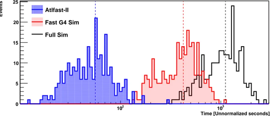
4.9 Distributions of CPU time for 250 t¯tevents in full, Fast G4, and ATLFAST-II simulations. Vertical dotted lines denote the aver-ages of the distributions. The Figure has been taken from [117]. 83
4.10 Fast simulations (color) and full simulation (black) compari-son of missing transverse energy along the x-axis in di-jet events with a leading parton pT between 560 and 1120 GeV (a) and of jet pT resolution as a function of pseudorapidity in t¯tevents
for jets with 20 < ptrue
T < 40 GeV (b). The Figures have been
taken from [117]. . . 84
5.1 Sketch of the flow of tracks through the ambiguity solver. Fig-ure taken from [138]. . . 90
5.2 The average number of primary tracks per unit of angular area as a function of the angular distance from the jet axis. Data (dashed lines) and dijet MC (solid lines) samples are compared in bins of jet pT showing the high density in the cores of ener-getic jets. Figure taken from [138]. . . 91
5.3 The average number of shared pixel (a) and SCT (b) clusters on primary tracks are shown as a function of the angular distance of the track from the jet axis. Data (dashed lines) and dijet MC (solid lines) samples are compared in bins of jet pT. The rise in both populations at small distances from the jet axis is expected due to the increasingly dense environment. The Figures have been taken from [138]. . . 92
5.4 Single-track reconstruction efficiency is shown as (a) a func-tion of the initial particle’s pT when it is required that the
par-ent particle decays before the IBL for the decay products of a ρ, three- and five-prong τ and a B0and (b) versus the production
radius for the decay products of a three- and five-prong τ as well as a B0, where no requirement in imposed on the
produc-tion radius of stable charged particles. The Figures have been taken from [138]. . . 92
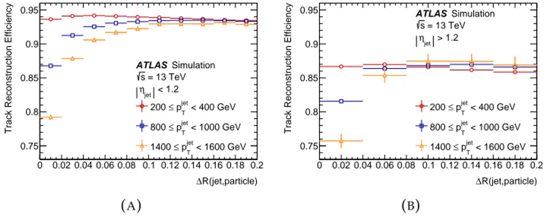
5.5 The efficiency to reconstruct charged primary particles in jets with (a) |η| < 1.2 and (b) |η| > 1.2 is shown as a function of the angular distance of the particle from the jet axis for various jet pT for simulated dijet MC events. The Figures have been taken
from [138]. . . 93
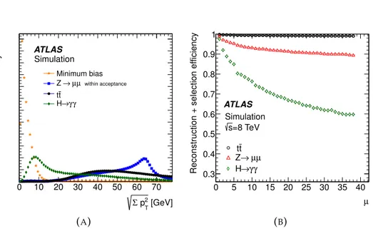
5.6 Contributions to the predicted primary vertex reconstruction efficiency as a function of the average number of interactions per bunch crossing, µ for the Higgs-boson decay into γγ (a), t¯tpair production leptonically decaying (b) and Z-boson to µµ decay (c). The black circles show the contribution to the effi-ciency from events categorised as clean, and the blue and red circles show the contributions from events with low and high pile-up contamination respectively. The open crosses show the sum of the contributions from events that are clean and those with low pile-up contamination; the filled crosses show the sum of the contributions from all categories and represent the overall efficiency, as shown in (d). The Figures have been taken from [144]. . . 96
5.7 (a): the distributions of the sum of the squared transverse mo-mentum for tracks from primary vertices, shown for simulated hard-scatter processes and a minimum-bias sample. (b): effi-ciency to reconstruct and then select the hard-scatter primary vertex as a function of µ, for different physics processes. The Figures have been taken from [144]. . . 97
5.8 Distribution of the average number of reconstructed vertices as a function of µ. (a): MC simulation of minimum-bias events (triangles) and the analytical function in Equation 5.2 fit to the simulation (solid line). The dashed curve shows the average estimated number of vertices lost to merging. (b): minimum-bias data (black points). The curve represents the result of the fit to the simulation after applying the µ-rescaling correc-tion. The inner dark (blue) band shows the systematic uncer-tainty in the fit from the beam-spot length, while the outer light (green) band shows the total uncertainty in the fit. The panels at the bottom of each figure represent the respective ra-tios of simulation or data to the fits described in the text. The Figures have been taken from [144]. . . 98
5.9 Schematic representation of the photon identification discrim-inating variables. ESN
C identifies the electromagnetic energy
collected in the N-th longitudinal layer of the electromagnetic calorimeter in a cluster of properties C, identifying the num-ber and/or properties of selected cells. Ei is the energy in the
i-th cell, ηithe pseudorapidity center of that cell. Figure taken
5.10 Comparison of the data-driven measurements of the identifi-cation efficiency for converted (a) and unconverted (b) pho-tons as a function of ET, for the |η| < 0.6 pseudorapidity
inter-val. The error bars represent the sum in quadrature of the sta-tistical and systematic uncertainties estimated in each method. The shaded areas correspond to the statistical uncertainties. The Figures have been taken from [149]. . . 103
5.11 Comparison of the measurements of the data-driven identi-fication efficiency for converted (a) and unconverted (b) pho-tons measurements obtained using the radiative Z method with the predictions from Z → llγ simulation as a function of pho-ton ET, for the |η| < 0.6 pseudorapidity interval. Predictions
are shown for both the nominal simulation and with the cor-rections applied. The bottom panels show the ratio of the data-driven values to the MC predictions. The Figures have been taken from [149]. . . 104
5.12 Comparison of the measurements of the data-driven identifi-cation efficiency for converted (a) and unconverted (b) pho-tons obtained using the electron extrapolation and inclusive photon methods with the predictions from prompt-photon+jet simulation as a function of photon ET, for the |η| < 0.6
pseu-dorapidity interval. Predictions are shown for both the nom-inal simulation and with the corrections applied. The bottom panels show the ratio of the data-driven values to the MC pre-dictions. The Figures have been taken from [149]. . . 104
5.13 Efficiency scale factors (SF) for each method and their combi-nation for converted (a) and unconverted (b) photons, for the |η| < 0.6 pseudorapidity interval. The Figures have been taken from [149]. . . 105
5.14 The efficiency to identify electrons from Z → ee decays (a) and the efficiency to identify hadrons as electrons (background re-jection) (b) estimated using simulated di-jet samples. The effi-ciencies are obtained using Monte Carlo simulations, and are measured with respect to reconstructed electrons. The Figures have been taken from [161]. . . 106
5.15 Combined electron reconstruction and identification efficien-cies in Z → ee events as a function of ET, integrated over the
full pseudorapidity range (a), and as a function of η, integrated over the full ET range (b). Two sets of uncertainties are shown:
the inner error bars show the statistical uncertainty, the outer error bars show the combined statistical and systematic uncer-tainty. The Figures have been taken from [161]. . . 108
5.16 Muon reconstruction efficiency as a function of η measured in Z → µµ events for muons with pT > 10 GeV shown for the
Medium muon selection for the Loose selection (squares) in the region |η| < 0.1, where the Loose and Medium selections dif-fer significantly (a), for the Tight muon selection (b) and for the High-pT uon selection (c). The error bars on the
efficien-cies indicate the statistical uncertainty. Panels at the bottom show the ratio of the measured to predicted efficiencies, with statistical and systematic uncertainties. The Figures have been taken from [164]. . . 111
5.17 Tau identification efficiency scale factors for one track and three track τ had-vis candidates with pT > 20 GeV. The combined
systematic and statistical uncertainties are shown. Figure taken from [167]. . . 114
5.18 Calibration stages for EM-scale jets. Other than the origin cor-rection, each stage of the calibration is applied to the four-momentum of the jet. Figure taken from [174]. . . 115
5.19 Combined uncertainty in the JES of fully calibrated jets as a function of jet pT at η = 0 (a) and η at pT = 80 GeV (b). The
Figures have been taken from [177]. . . 119
5.20 (a): The MV2c10 output for b-jets (solid line), c-jets (dashed line) and light-flavour jets (dotted line) in simulated t¯tevents. (b): The light-flavour jet (dashed line) and c-jet rejection fac-tors (solid line) as a function of the b-jet tagging efficiency of the MV2c10 b-tagging algorithm. The Figures have been taken from [179]. . . 121
5.21 The light-flavour jet (squares) and c-jet rejection factors (tri-angles) at a b-tagging efficiency of 70% single-cut OP (a) and flat-efficiency OP (b) as a function of the jet pT for the MV2c10
b-tagging algorithms in t¯tevents. The Figures have been taken from [179]. . . 122
5.22 The b-jet tagging efficiency measured in data (full circles) and simulation (open circles), corresponding to the 70% b-jet tag-ging efficiency single-cut OP, as a function of the jet pT using
the T&P (a) and the LH method (b), for R=0.4 calorimeter-jets. The error bars correspond to the total statistical and systematic uncertainties. The Figures have been taken from [179]. . . 124
5.23 Data-to-simulation scale factors, corresponding to the 70% b-jet tagging efficiency single-cut OP, as a function of the b-jet |η| using the T&P (a) and the LH method (b) for R=0.4 calorimeter-jets. Both the statistical uncertainties (error bars) and total un-certainties (shaded region) are shown. The Figures have been taken from [179]. . . 124
5.24 Fake rate from pile up jets versus hard-scatter jet efficiency curves for JVF, corrJVF, RpT, and JVT. The widely used JVF
working points with cut values 0.25 and 0.5 are indicated with gold and green stars. Figure taken from [183].. . . 128
5.25 Distributions of the Emiss
T resolution versus NP V for ETmissbuilt
with three different forward jet selections in a Z → µµ (a) and VBF H → W W (b) simulation. The Figures have been taken from [187]. . . 130
5.26 Sketch of the track-based soft term projections with respect to phard
T for the calculation of the TST systematic uncertainties.
Figure taken from [187]. . . 131
5.27 Parallel resolution plots for the EMTopo TST for the jet-inclusive (a) and jet-veto (b) selections. Analougously, the resoluton plots for the PFlow TST are shown in (c) and (d), respectively. The pink band, centered on data, represents the resulting system-atic uncertainty applied to the Z → ee MC simulation. The Figures have been taken from [187]. . . 132
5.28 The RMS obtained from the combined distributions of EM-Topo Emiss
x and Eymissfor data with EMTopo jets (circular marker)
and PFlow jets (triangular marker) and MC simulation with EMTopo jets (square marker) in a Z → ee event selection. The resolutions are shown using the Loose Emiss
T WP are shown
versus < µ > (a) and NP V (b). The same distributions for the
Tight Emiss
T WP are shown in (c) and (d), respectively. The pink
band indicates the size of the detector level systematic uncer-tainties. The Figures have been taken from [187]. . . 133
6.1 Pictorical representation of a top-antitop quark pair decaying into the fully hadronic channel. The red blob in the center repre-sents the hard-scatter collision. Light-quark (b-quark) initiated jets are represented by purple (yellow) cones. . . 136
6.2 Mass spectra at detector level of the W boson (a) and top quark (c), determined from parton-matched jets. The particle level re-sults are shown in (b) and (d), respectively. The fitted gaussian is shown in red, with the peak and width parameters shown.. 146
6.3 Distributions of observables used for background rejection, shown in data, non all hadronic t¯t and signal for events preselected as in Section 6.4. The variables shown are the χ2
discrimi-nant 6.3a, ∆Rbb(b), ∆RmaxbW (c) and mtop (d), filled for both top
quark candidates in each event. Cut values are indicated by red dashed lines. . . 147
6.4 Distributions of observables used for background rejection, shown in data, non all hadronic t¯t and signal with all selection cuts applied with the exception of the cut on the variable being shown. The variables shown are the χ2discriminant (a), ∆R
bb(b),
∆RmaxbW (c) and mtop (d), filled for both top quark candidates in
each event. Cut values are indicated by red dashed lines. . . . 148
6.5 MC-subtracted data distribution of mt in exclusive nb−jets regions.
6.6 Reconstructed level distribution in the signal regions as a function of
σt¯t. The signal prediction (open histogram) is based on the Powheg+Pythia8
generator. The background is the sum of the data-driven multijet estimate (purple histogram) and the MC-based expectation for the
contributions of non all-hadronic t¯t production process (light blue
histogram). The shaded area represents the total statistical and
sys-tematic uncertainties. . . 154
6.7 Reconstructed level distributions in the signal regions as a function
of ptop1T for particle (a) and parton level (b) optimized binning and
as a function of ptop2T for particle (c) and parton level (d) optimized binning. The signal prediction (open histogram) is based on the Powheg+Pythia8 generator. The background is the sum of the data-driven multijet estimate (purple histogram) and the MC-based
ex-pectation for the contributions of non all-hadronic t¯tproduction
pro-cess (light blue histogram). The shaded area represents the total
sta-tistical and systematic uncertainties. . . 155
6.8 Reconstructed level distributions in the signal regions as a function
of ytop1 for particle (a) and parton level (b) optimized binning and
as a function of ytop2for particle (c) and parton level (d) optimized
binning. The signal prediction (open histogram) is based on the Powheg+Pythia8 generator. The background is the sum of the data-driven multijet estimate (purple histogram) and the MC-based
ex-pectation for the contributions of non all-hadronic t¯tproduction
pro-cess (light blue histogram). The shaded area represents the total
sta-tistical and systematic uncertainties. . . 156
6.9 Reconstructed level distributions in the signal regions as a function
of pt¯Tt for particle (a) and parton level (b) optimized binning and
as a function of yt¯t for particle (c) and parton level (d) optimized
binning. The signal prediction (open histogram) is based on the Powheg+Pythia8 generator. The background is the sum of the data-driven multijet estimate (purple histogram) and the MC-based
ex-pectation for the contributions of non all-hadronic t¯tproduction
pro-cess (light blue histogram). The shaded area represents the total
sta-tistical and systematic uncertainties. . . 157
6.10 Reconstructed level distributions in the signal regions as a function
of mt¯tfor particle (a) and parton level (b) optimized binning. The
signal prediction (open histogram) is based on the Powheg+Pythia8 generator. The background is the sum of the data-driven multijet estimate (purple histogram) and the MC-based expectation for the
contributions of non all-hadronic t¯t production process (light blue
histogram). The shaded area represents the total statistical and
6.11 Reconstructed level distributions in the signal regions as a function of Njets (a), ∆φt¯t (b), |Poutt¯t | (c) and HTt¯t (d). The signal prediction
(open histogram) is based on the Powheg+Pythia8 generator. The background is the sum of the data-driven multijet estimate (purple histogram) and the MC-based expectation for the contributions of
non all-hadronic t¯tproduction process (light blue histogram). The
shaded area represents the total statistical and systematic uncertainties.159
6.12 Reconstructed level distributions in the signal regions as a function
of RWb1 (a), RWb2 (b), RWt1 (c) and RWt2 (d). The signal prediction (open histogram) is based on the Powheg+Pythia8 generator. The back-ground is the sum of the data-driven multijet estimate (purple his-togram) and the MC-based expectation for the contributions of non
all-hadronic t¯tproduction process (light blue histogram). The shaded
area represents the total statistical and systematic uncertainties. . . 160
6.13 Reconstructed level distributions in the signal regions as a function
of ∆Rtopextra1 (a), ∆Rjet1extra1 (b), Rtop1extra1 (c) and Rjet1extra1 (d). The
sig-nal prediction (open histogram) is based on the Powheg+Pythia8 generator. The background is the sum of the data-driven multijet estimate (purple histogram) and the MC-based expectation for the
contributions of non all-hadronic t¯t production process (light blue
histogram). The shaded area represents the total statistical and
sys-tematic uncertainties. . . 161
7.1 The acceptance and efficiency corrections for the ptop1T spec-trum at particle ( (a) and (b), respectively) and parton level ( (c) and (d), respectively). The corrections are obtained from the nominal fully hadronic t¯tMC sample. . . 166
7.2 The migration matrices from reconstruction to particle (a) and reconstruction to parton levels (b) for the ptop1T spectrum. The corrections are obtained from the nominal fully hadronic t¯t MC sample. . . 167
7.3 Unfolding to particle (a) and parton (b) level closure test of the
dif-ferential cross section as a function of ptop1T ; the observable is nor-malised in the fiducial phase-space. The shaded area represents the
statistical uncertainty. . . 168
7.4 Linearity stress test using for the normalised cross section as a
func-tion of ptop1T . The stress is achieve by re-weigthing the input distri-bution (red line) by a factor proportional to the data/MC difference. The particle level results have used a factor of 1 (a) or 5 (b). The
cor-responding parton level results are shown in (c) and (d), respectively. 169
7.5 χ2 (a) between the unfolded result and the prior of the i − th
itera-tion of unfolding to particle level as a funcitera-tion of the Niterfor ptop1T .
Figures (b), (c) and (d) show the statistical error, the residuals (w.r.t. previous iteration) and their ratio for the fifth bin of ptop1T , respectively.171
8.1 Fractional uncertainties in the fiducial phase space as a function of
|Pt¯t
out|: absolute (a) and normalised (b). The shaded area represents
8.2 Fractional uncertainties in the fiducial phase space as a function of
∆φt¯t: absolute (a) and normalised (b). The shaded area represents
the total statistical and systematic uncertainties. . . 178
8.3 Fractional uncertainties in the fiducial phase space as a function of
∆Rjet1extra1: absolute (a) and normalised (b). The shaded area
repre-sents the total statistical and systematic uncertainties. . . 179
8.4 Fractional uncertainties in the fiducial phase space as a function of
∆Rtopcloseextra1 : absolute (a) and normalised (b). The shaded area
repre-sents the total statistical and systematic uncertainties. . . 179
8.5 Fractional uncertainties in the fiducial phase space as a function of
HTt¯t: absolute (a) and normalised (b). The shaded area represents the
total statistical and systematic uncertainties. . . 180
8.6 Fractional uncertainties in the fiducial phase space as a function of
number of jets: absolute (a) and normalised (b). The shaded area
represents the total statistical and systematic uncertainties. . . 180
8.7 Fractional uncertainties in the fiducial phase space as a function of
Rjet1extra1: absolute (a) and normalised (b). The shaded area represents
the total statistical and systematic uncertainties. . . 181
8.8 Fractional uncertainties in the fiducial phase space as a function of
Rtop1extra1: absolute (a) and normalised (b). The shaded area represents
the total statistical and systematic uncertainties. . . 181
8.9 Fractional uncertainties in the fiducial phase space as a function of
RleadingW b : absolute (a) and normalised (b). The shaded area represents
the total statistical and systematic uncertainties. . . 182
8.10 Fractional uncertainties in the fiducial phase space as a function of
RsubleadingW b : absolute (a) and normalised (b). The shaded area
repre-sents the total statistical and systematic uncertainties. . . 182
8.11 Fractional uncertainties in the fiducial phase space as a function of
RleadingW t : absolute (a) and normalised (b). The shaded area represents
the total statistical and systematic uncertainties. . . 183
8.12 Fractional uncertainties in the fiducial phase space as a function of
RsubleadingW t : absolute (a) and normalised (b). The shaded area
repre-sents the total statistical and systematic uncertainties. . . 183
8.13 Fractional uncertainties in the fiducial phase space as a function of
ptop1T : absolute (a) and normalised (b). The shaded area represents
the total statistical and systematic uncertainties. . . 184
8.14 Fractional uncertainties in the fiducial phase space as a function of
ytop1: absolute (a) and normalised (b). The shaded area represents
the total statistical and systematic uncertainties. . . 184
8.15 Fractional uncertainties in the fiducial phase space as a function of
ptop2T : absolute (a) and normalised (b). The shaded area represents
the total statistical and systematic uncertainties. . . 185
8.16 Fractional uncertainties in the fiducial phase space as a function of
ytop2: absolute (a) and normalised (b). The shaded area represents
8.17 Fractional uncertainties in the fiducial phase space as a function of
mt¯t: absolute (a) and normalised (b). The shaded area represents the
total statistical and systematic uncertainties. . . 186
8.18 Fractional uncertainties in the fiducial phase space as a function of
pt¯Tt: absolute (a) and normalised (b). The shaded area represents the
total statistical and systematic uncertainties. . . 186
8.19 Fractional uncertainties in the fiducial phase space as a function of
yt¯t: absolute (a) and normalised (b). The shaded area represents the
total statistical and systematic uncertainties. . . 187
8.20 Fractional uncertainties in the full phase space as a function of ptop1T : absolute (a) and normalised (b). The shaded area represents the total
statistical and systematic uncertainties. . . 188
8.21 Fractional uncertainties in the full phase space as a function of ytop1:
absolute (a) and normalised (b). The shaded area represents the total
statistical and systematic uncertainties. . . 188
8.22 Fractional uncertainties in the full phase space as a function of ptop2T : absolute (a) and normalised (b). The shaded area represents the total
statistical and systematic uncertainties. . . 189
8.23 Fractional uncertainties in the full phase space as a function of ytop2:
absolute (a) and normalised (b). The shaded area represents the total
statistical and systematic uncertainties. . . 189
8.24 Fractional uncertainties in the full phase space as a function of mt¯t:
absolute (a) and normalised (b). The shaded area represents the total
statistical and systematic uncertainties. . . 190
8.25 Fractional uncertainties in the full phase space as a function of pt¯Tt: absolute (a) and normalised (b). The shaded area represents the total
statistical and systematic uncertainties. . . 190
8.26 Fractional uncertainties in the full phase space as a function of yt¯t:
absolute (a) and normalised (b). The shaded area represents the total
statistical and systematic uncertainties. . . 191
9.1 Differential cross sections in the fiducial phase space as a function of
|Pt¯t
out|: absolute (a) and normalised (b). The shaded area represents
the total statistical and systematic uncertainties. . . 193
9.2 Differential cross sections in the fiducial phase space as a function of
∆φt¯t: absolute (a) and normalised (b). The shaded area represents
the total statistical and systematic uncertainties. . . 193
9.3 Differential cross sections in the fiducial phase space as a function of
∆Rjet1extra1: absolute (a) and normalised (b). The shaded area
repre-sents the total statistical and systematic uncertainties. . . 194
9.4 Differential cross sections in the fiducial phase space as a function of
∆Rtopcloseextra1 : absolute (a) and normalised (b). The shaded area
repre-sents the total statistical and systematic uncertainties. . . 194
9.5 Differential cross sections in the fiducial phase space as a function of
HTt¯t: absolute (a) and normalised (b). The shaded area represents the
9.6 Differential cross sections in the fiducial phase space as a function of number of jets: absolute (a) and normalised (b). The shaded area
represents the total statistical and systematic uncertainties. . . 195
9.7 Differential cross sections in the fiducial phase space as a function of
Rjet1extra1: absolute (a) and normalised (b). The shaded area represents
the total statistical and systematic uncertainties. . . 196
9.8 Differential cross sections in the fiducial phase space as a function of
Rtop1extra1: absolute (a) and normalised (b). The shaded area represents
the total statistical and systematic uncertainties. . . 196
9.9 Differential cross sections in the fiducial phase space as a function of
RleadingW b : absolute (a) and normalised (b). The shaded area represents
the total statistical and systematic uncertainties. . . 197
9.10 Differential cross sections in the fiducial phase space as a function of
RsubleadingW b : absolute (a) and normalised (b). The shaded area
repre-sents the total statistical and systematic uncertainties. . . 197
9.11 Differential cross sections in the fiducial phase space as a function of
RleadingW t : absolute (a) and normalised (b). The shaded area represents
the total statistical and systematic uncertainties. . . 198
9.12 Differential cross sections in the fiducial phase space as a function of
RsubleadingW t : absolute (a) and normalised (b). The shaded area
repre-sents the total statistical and systematic uncertainties. . . 198
9.13 Differential cross sections in the fiducial phase space as a function of
ptop1T : absolute (a) and normalised (b). The shaded area represents
the total statistical and systematic uncertainties. . . 199
9.14 Differential cross sections in the fiducial phase space as a function of
ytop1: absolute (a) and normalised (b). The shaded area represents
the total statistical and systematic uncertainties. . . 199
9.15 Differential cross sections in the fiducial phase space as a function of
ptop2T : absolute (a) and normalised (b). The shaded area represents
the total statistical and systematic uncertainties. . . 200
9.16 Differential cross sections in the fiducial phase space as a function of
ytop2: absolute (a) and normalised (b). The shaded area represents
the total statistical and systematic uncertainties. . . 200
9.17 Differential cross sections in the fiducial phase space as a function of
mt¯t: absolute (a) and normalised (b). The shaded area represents the
total statistical and systematic uncertainties. . . 201
9.18 Differential cross sections in the fiducial phase space as a function of
pt¯Tt: absolute (a) and normalised (b). The shaded area represents the
total statistical and systematic uncertainties. . . 201
9.19 Differential cross sections in the fiducial phase space as a function of
yt¯t: absolute (a) and normalised (b). The shaded area represents the
total statistical and systematic uncertainties. . . 202
9.20 Differential cross sections in the full phase space as a function of
ptop1T : absolute (a) and normalised (b). The shaded area represents
9.21 Differential cross sections in the full phase space as a function of
ytop1: absolute (a) and normalised (b). The shaded area represents
the total statistical and systematic uncertainties. . . 203
9.22 Differential cross sections in the full phase space as a function of
ptop2T : absolute (a) and normalised (b). The shaded area represents
the total statistical and systematic uncertainties. . . 204
9.23 Differential cross sections in the full phase space as a function of
ytop2: absolute (a) and normalised (b). The shaded area represents
the total statistical and systematic uncertainties. . . 205
9.24 Differential cross sections in the full phase space as a function of mt¯t:
absolute (a) and normalised (b). The shaded area represents the total
statistical and systematic uncertainties. . . 206
9.25 Differential cross sections in the full phase space as a function of pt¯Tt: absolute (a) and normalised (b). The shaded area represents the total
statistical and systematic uncertainties. . . 208
9.26 Differential cross sections in the full phase space as a function of yt¯t:
absolute (a) and normalised (b). The shaded area represents the total
statistical and systematic uncertainties. . . 209
A.1 Detector- to particle-level migration matrices for the Ht¯Tt spectrum
in 4 different configuration: using the fitted resolutions at detector
and particle level and a fixed χ2 cut (a), imposing the detector level
resolution at particle level with a fixed χ2cut (b), using the fitted res-olutions at detector and particle level and a flat efficiency χ2 cut (c),
and imposing the detector level resolution at particle level with a flat
efficiency χ2cut (d). The relative differences are at 1% level. . . 213
A.2 Detector- to particle-level migration matrices for the |Pout| spectrum
in 4 different configuration: using the fitted resolutions at detector
and particle level and a fixed χ2 cut (a), imposing the detector level
resolution at particle level with a fixed χ2cut (b), using the fitted
res-olutions at detector and particle level and a flat efficiency χ2 cut (c), and imposing the detector level resolution at particle level with a flat
efficiency χ2cut (d). The relative differences are at 1% level. . . . . 214
A.3 Detector- to particle-level migration matrices for the pt¯Ttspectrum in 4 different configuration: using the fitted resolutions at detector and
particle level and a fixed χ2cut (a), imposing the detector level
res-olution at particle level with a fixed χ2cut (b), using the fitted reso-lutions at detector and particle level and a flat efficiency χ2 cut (c), and imposing the detector level resolution at particle level with a flat
efficiency χ2cut (d). The relative differences are at 1% level. . . 215
A.4 Detector- to particle-level migration matrices for the |yTt¯t| spectrum in 4 different configuration: using the fitted resolutions at detector
and particle level and a fixed χ2 cut (a), imposing the detector level
resolution at particle level with a fixed χ2cut (b), using the fitted res-olutions at detector and particle level and a flat efficiency χ2 cut (c),
and imposing the detector level resolution at particle level with a flat
E.1 (a) Acceptance correction,(b) efficiency and (c) reconstruction-to-particle-level migration matrix for |Pt¯t
out| observable. . . 269
E.2 (a) Acceptance correction,(b) efficiency and (c)
reconstruction-to-particle-level migration matrix for ∆φt¯tobservable. . . 270
E.3 (a) Acceptance correction,(b) efficiency and (c)
reconstruction-to-particle-level migration matrix for ∆Rjet1extra1observable. . . 271
E.4 (a) Acceptance correction,(b) efficiency and (c)
reconstruction-to-particle-level migration matrix for ∆Rextra1
topcloseobservable. . . 272
E.5 (a) Acceptance correction,(b) efficiency and (c)
reconstruction-to-particle-level migration matrix for HTt¯tobservable. . . 273
E.6 (a) Acceptance correction,(b) efficiency and (c)
reconstruction-to-particle-level migration matrix for N. jets observable. . . 274
E.7 (a) Acceptance correction,(b) efficiency and (c)
reconstruction-to-particle-level migration matrix for Rextra1
jet1 observable. . . 275
E.8 (a) Acceptance correction,(b) efficiency and (c)
reconstruction-to-particle-level migration matrix for Rtop1extra1observable. . . 276
E.9 (a) Acceptance correction,(b) efficiency and (c)
reconstruction-to-particle-level migration matrix for RleadingW b observable. . . 277
E.10 (a) Acceptance correction,(b) efficiency and (c)
reconstruction-to-particle-level migration matrix for RsubleadingW b observable. . . 278
E.11 (a) Acceptance correction,(b) efficiency and (c)
reconstruction-to-particle-level migration matrix for RleadingW t observable. . . 279
E.12 (a) Acceptance correction,(b) efficiency and (c)
reconstruction-to-particle-level migration matrix for RsubleadingW t observable. . . 280
E.13 (a) Acceptance correction,(b) efficiency and (c)
reconstruction-to-particle-level migration matrix for ptop1T observable. . . 281
E.14 (a) Acceptance correction,(b) efficiency and (c)
reconstruction-to-particle-level migration matrix for ytop1observable. . . 282
E.15 (a) Acceptance correction,(b) efficiency and (c)
reconstruction-to-particle-level migration matrix for ptop2T observable. . . 283
E.16 (a) Acceptance correction,(b) efficiency and (c)
reconstruction-to-particle-level migration matrix for ytop2observable. . . 284
E.17 (a) Acceptance correction,(b) efficiency and (c)
reconstruction-to-particle-level migration matrix for mt¯tobservable. . . 285
E.18 (a) Acceptance correction,(b) efficiency and (c)
reconstruction-to-particle-level migration matrix for pt¯Ttobservable. . . 286
E.19 (a) Acceptance correction,(b) efficiency and (c)
reconstruction-to-particle-level migration matrix for yt¯tobservable. . . 287
E.20 (a) Acceptance correction,(b) efficiency and (c)
reconstruction-to-parton-level migration matrix for ptop1T observable. . . 288
E.21 (a) Acceptance correction,(b) efficiency and (c)
reconstruction-to-parton-level migration matrix for ytop1observable. . . 289
E.22 (a) Acceptance correction,(b) efficiency and (c)
reconstruction-to-parton-level migration matrix for ptop2T observable. . . 290
E.23 (a) Acceptance correction,(b) efficiency and (c)
E.24 (a) Acceptance correction,(b) efficiency and (c) reconstruction-to-parton-level migration matrix for pt¯t
T observable. . . 292
E.25 (a) Acceptance correction,(b) efficiency and (c)
reconstruction-to-parton-level migration matrix for yt¯tobservable. . . 293
F.1 Unfolding closure of a differential cross-section as a function of ptop1T (a), ytop1(b), ptop2T (c) and ytop2(d) observables normalised in the fiducial
phase-space. The shaded area represents the statistical uncertainty.. 295
F.2 Unfolding closure of a differential cross-section as a function of pt¯t
T (a),
yt¯t(b) and mt¯t(c) observables normalised in the fiducial phase-space.
The shaded area represents the statistical uncertainty. . . 296
F.3 Unfolding closure of a differential cross-section as a function of |Pt¯t out| (a),
∆φt¯t(b), HTt¯t(c) and Njets (d) observables normalised in the fiducial
phase-space. The shaded area represents the statistical uncertainty.. 297
F.4 Unfolding closure of a differential cross-section as a function of ∆Rextra1
jet1 (b),
∆Rtopcloseextra1 (c), Rjet1extra1(a) and Rtop1extra1(d) observables normalised in
the fiducial phase-space. The shaded area represents the statistical
uncertainty. . . 298
F.5 Unfolding closure of a differential cross-section as a function of RleadingW b (a),
RsubleadingW b (b), RleadingW t (c) and RsubleadingW t (d) observables normalised
in the fiducial phase-space. The shaded area represents the statistical
uncertainty. . . 299
F.6 Unfolding closure of a differential cross-section as a function of the
pt,1T (a), yt,1(b), pt,2
T (c) and yt,2 (d) observables normalised in the full
phase-space. The shaded area represents the statistical uncertainty.. 300
F.7 Unfolding closure of a differential cross-section as a function of the
mt¯t (a), pt¯t
T (b) and yt¯t (c) observable normalised in the full
phase-space. The shaded area represents the statistical uncertainty. . . 301
F.8 Linearity stress test using for the normalised cross section as a
func-tion of |Pt¯t
out|. The stress is achieve by re-weigthing the input
distri-bution (red line) by a factor proportional to the data/MC difference. The factors are 1 (top left), 2 (top right), 3 (center left), 4 (center right),
5 (bottom). The efficiency correction has been applied. . . 302
F.9 Linearity stress test using for the normalised cross section as a
func-tion of ∆φt¯t. The stress is achieve by re-weigthing the input
distri-bution (red line) by a factor proportional to the data/MC difference. The factors are 1 (top left), 2 (top right), 3 (center left), 4 (center right),
5 (bottom). The efficiency correction has been applied. . . 303
F.10 Linearity stress test using for the normalised cross section as a
func-tion of ∆Rjet1extra1. The stress is achieve by re-weigthing the input
distribution (red line) by a factor proportional to the data/MC dif-ference. The factors are 1 (top left), 2 (top right), 3 (center left), 4
(center right), 5 (bottom). The efficiency correction has been applied. 304
F.11 Linearity stress test using for the normalised cross section as a
func-tion of ∆Rextra1
topclose. The stress is achieve by re-weigthing the input
distribution (red line) by a factor proportional to the data/MC dif-ference. The factors are 1 (top left), 2 (top right), 3 (center left), 4
F.12 Linearity stress test using for the normalised cross section as a func-tion of Ht¯t
T. The stress is achieve by re-weigthing the input
distri-bution (red line) by a factor proportional to the data/MC difference. The factors are 1 (top left), 2 (top right), 3 (center left), 4 (center right),
5 (bottom). The efficiency correction has been applied. . . 306
F.13 Linearity stress test using for the normalised cross section as a
func-tion of number of jets. The stress is achieve by re-weigthing the input distribution (red line) by a factor proportional to the data/MC dif-ference. The factors are 1 (top left), 2 (top right), 3 (center left), 4
(center right), 5 (bottom). The efficiency correction has been applied. 307
F.14 Linearity stress test using for the normalised cross section as a
func-tion of Rjet1extra1. The stress is achieve by re-weigthing the input distri-bution (red line) by a factor proportional to the data/MC difference. The factors are 1 (top left), 2 (top right), 3 (center left), 4 (center right),
5 (bottom). The efficiency correction has been applied. . . 308
F.15 Linearity stress test using for the normalised cross section as a
func-tion of Rextra1
top1 . The stress is achieve by re-weigthing the input
distri-bution (red line) by a factor proportional to the data/MC difference. The factors are 1 (top left), 2 (top right), 3 (center left), 4 (center right),
5 (bottom). The efficiency correction has been applied. . . 309
F.16 Linearity stress test using for the normalised cross section as a
func-tion of RleadingW b . The stress is achieve by re-weigthing the input distri-bution (red line) by a factor proportional to the data/MC difference. The factors are 1 (top left), 2 (top right), 3 (center left), 4 (center right),
5 (bottom). The efficiency correction has been applied. . . 310
F.17 Linearity stress test using for the normalised cross section as a
func-tion of RsubleadingW b . The stress is achieve by re-weigthing the input distribution (red line) by a factor proportional to the data/MC dif-ference. The factors are 1 (top left), 2 (top right), 3 (center left), 4
(center right), 5 (bottom). The efficiency correction has been applied. 311
F.18 Linearity stress test using for the normalised cross section as a
func-tion of RleadingW t . The stress is achieve by re-weigthing the input distri-bution (red line) by a factor proportional to the data/MC difference. The factors are 1 (top left), 2 (top right), 3 (center left), 4 (center right),
5 (bottom). The efficiency correction has been applied. . . 312
F.19 Linearity stress test using for the normalised cross section as a
func-tion of RsubleadingW t . The stress is achieve by re-weigthing the input distribution (red line) by a factor proportional to the data/MC dif-ference. The factors are 1 (top left), 2 (top right), 3 (center left), 4
(center right), 5 (bottom). The efficiency correction has been applied. 313
F.20 Linearity stress test using for the normalised cross section as a
func-tion of ptop1T . The stress is achieve by re-weigthing the input distri-bution (red line) by a factor proportional to the data/MC difference. The factors are 1 (top left), 2 (top right), 3 (center left), 4 (center right),
F.21 Linearity stress test using for the normalised cross section as a
func-tion of ytop1. The stress is achieve by re-weigthing the input
distri-bution (red line) by a factor proportional to the data/MC difference. The factors are 1 (top left), 2 (top right), 3 (center left), 4 (center right),
5 (bottom). The efficiency correction has been applied. . . 315
F.22 Linearity stress test using for the normalised cross section as a
func-tion of ptop2T . The stress is achieve by re-weigthing the input distri-bution (red line) by a factor proportional to the data/MC difference. The factors are 1 (top left), 2 (top right), 3 (center left), 4 (center right),
5 (bottom). The efficiency correction has been applied. . . 316
F.23 Linearity stress test using for the normalised cross section as a
func-tion of ytop2. The stress is achieve by re-weigthing the input
distri-bution (red line) by a factor proportional to the data/MC difference. The factors are 1 (top left), 2 (top right), 3 (center left), 4 (center right),
5 (bottom). The efficiency correction has been applied. . . 317
F.24 Linearity stress test using for the normalised cross section as a
func-tion of mt¯t. The stress is achieve by re-weigthing the input
distri-bution (red line) by a factor proportional to the data/MC difference. The factors are 1 (top left), 2 (top right), 3 (center left), 4 (center right),
5 (bottom). The efficiency correction has been applied. . . 318
F.25 Linearity stress test using for the normalised cross section as a
func-tion of pt¯Tt. The stress is achieve by re-weigthing the input distri-bution (red line) by a factor proportional to the data/MC difference. The factors are 1 (top left), 2 (top right), 3 (center left), 4 (center right),
5 (bottom). The efficiency correction has been applied. . . 319
F.26 Linearity stress test using for the normalised cross section as a
func-tion of yt¯t. The stress is achieve by re-weigthing the input
distri-bution (red line) by a factor proportional to the data/MC difference. The factors are 1 (top left), 2 (top right), 3 (center left), 4 (center right),
5 (bottom). The efficiency correction has been applied. . . 320
F.27 Linearity stress test using for the normalised cross section as a
func-tion of ptop1T . The stress is achieve by re-weigthing the input distri-bution (red line) by a factor proportional to the data/MC difference. The factors are 1 (top left), 2 (top right), 3 (center left), 4 (center right),
5 (bottom). The efficiency correction has been applied. . . 322
F.28 Linearity stress test using for the normalised cross section as a
func-tion of ytop1. The stress is achieve by re-weigthing the input
distri-bution (red line) by a factor proportional to the data/MC difference. The factors are 1 (top left), 2 (top right), 3 (center left), 4 (center right),
5 (bottom). The efficiency correction has been applied. . . 323
F.29 Linearity stress test using for the normalised cross section as a
func-tion of ptop2T . The stress is achieve by re-weigthing the input distri-bution (red line) by a factor proportional to the data/MC difference. The factors are 1 (top left), 2 (top right), 3 (center left), 4 (center right),
![Figure 1.2 shows a recent ATLAS measurement [ 16 ] of α s at different values](https://thumb-eu.123doks.com/thumbv2/123dokorg/2868469.9192/44.892.144.710.463.837/figure-shows-recent-atlas-measurement-a-different-values.webp)