EUI
WORKING
PAPERS IN
ECONOMICS
EU I Working Paper EC O No. 93/31
An Application of the Kalman Filter to the Spanish Experience in a Target Zone (1989-92)
Enrique Alberola Ila J. Humberto Lopez Vicente Orts Rio s © The Author(s). European University Institute. version produced by the EUI Library in 2020. Available Open Access on Cadmus, European University Institute Research Repository.
© The Author(s). European University Institute. version produced by the EUI Library in 2020. Available Open Access on Cadmus, European University Institute Research Repository.
EUROPEAN UNIVERSITY INSTITUTE, FLORENCE ECONOMICS DEPARTMENT
EUI Working Paper EC O No. 93/31
An Application of the Kalman Filter to the Spanish Experience in a Target Zone (1989-92)
Enrique Alberola Ila
J. Humberto Lopez
Vicente Orts Rios
BADIA FIESOLANA, SAN DOMENICO (FI)
© The Author(s). European University Institute. version produced by the EUI Library in 2020. Available Open Access on Cadmus, European University Institute Research Repository.
All rights reserved.
No part of this paper may be reproduced in any form without permission of the authors.
© Enrique Alberola Ila, J. Humberto Lopez, Vicente Orts Rios Printed in Italy in October 1993
European University Institute Badia Fiesolana I - 50016 San Domenico (FI)
Italy © The Author(s). European University Institute. version produced by the EUI Library in 2020. Available Open Access on Cadmus, European University Institute Research Repository.
An application of the Kalman Filter to the Spanish
experience in a target zone (1989-92)
Enrique Alberala Ila, J. Humberto Lopez
Economics Department. Istituto Universitario Europeo, Firenze
Vicente Orts Rios
Departamento de Analisis Economico.Universidad de Valencia This version: October 1993
Abstract
This work presents an empirical analysis of the evolution of the Spanish peseta in the EMS. Previously, the basic target zone model is explained and some extensions introduced. These extensions are the consideration of devaluation risks, capital controls and the possibility of sterilized interventions. The empirical part consists in applying a Kalman filter to the series to obtain an unobserved components decomposition for the interest rate differentials. The empirical evidence does not support the target zone model for Spain: the interest rate differentials have largely reflected realignment risks, rather than exchange rate expectations within the band.
We are grateful to M. Salmon, F. Canova and A. Maravall for their many useful comments. Special thanks are also due to our colleagues S. Fabrizio, J. Stanton-Ife and L. Gomez. E. Alberala gratefully acknowledges financial support from Fundacion Ramon Areces. © The Author(s). European University Institute. version produced by the EUI Library in 2020. Available Open Access on Cadmus, European University Institute Research Repository.
■ © The Author(s). European University Institute. version produced by the EUI Library in 2020. Available Open Access on Cadmus, European University Institute Research Repository.
Introduction
This paper studies the evidence of the target-zone models for Spain from the entry of the peseta in the European Monetary System (EMS) until its first realignment, covering a period over three years. We apply the Kalman filter to a linear approximation of the theoretical target zone model in order to obtain an unobserved components decomposition for the interest rate differentials.
Section I briefly develops the basic target zone model and discusses some
extensions: introduction of a devaluation risk, capital controls and the possibility of sterilized interventions; these considerations may interfere with the basic theoretical relation in practice. Actually, the outcome of the empirical analysis carried out in
section II does not support the basic model; once the extensions-conveyed in a single
parameter (c,)- are considered, the target zone is not found to influence the interest differentials, as the theory would predict. Section III interprets the results and stresses the importance of the credibility component to explain the gap in the interest rate differentials. The conclusions summarize the results and provide an explanation for the evolution of the realignment risk, highlighting the reasons which led to the first realignment of the peseta in the EMS.
I-Target-zone basic model and extensions
The disciplinary mechanism of the EMS is the most outstanding example of target zone. The rules of the EMS imply the intervention of the central banks of the system to defend the band around an institutionally-fixed central parity1. Consequently the EMS is a system of semifixed but adjustable exchange rates, which can be studied in the framework of the target-zone models, which were first proposed by Krugman (1990).
From a simple monetary model of exchange rate determination in which the Interest Parity Condition (IP) holds in the strong form of the Uncovered Parity (UCP), we obtain the known result that the current level of exchange rate (s,) depends both on economic factors-fundamentals (/,)-and on the expectations of the future exchange rate, which are in turn determined by the future expected value of the fundamentals:
ds s - f + 6 E __I
' ' ' 1 dt [U
where (5 is the semielasticity of the demand of money to the interest rate and
For details about the functioning of the EMS see, for instance, Giavazzi & Giovaninni (1989), ch. 1,2. 1 © The Author(s). European University Institute. version produced by the EUI Library in 2020. Available Open Access on Cadmus, European University Institute Research Repository.
Srv,+m,
vr m;.W(y; y ) [21
m being the (log) money supply and y the (log) level of output. The asterisks indicate foreign country's variables and the model is expressed in continuous time. It is convenient to make the above separation in the definition of the fundamentals, for the money supply constitutes the policy instrument in this framework2.
Assumming that the changes in f (df) follow a Brownian motion, with drift i±:
the exchange rate in a free float regime-that is when the fundamentals are not constrained - is simply:
where the expectation equals the drift. This yields the solid 45-degrees line in Fig l.B. However, in a target zone the monetary authorities are expected to defend the band through interventions at the edges of the band (marginal interventions), constraining the behaviour of the fundamentals, which now follow a regulated Brownian motion of the type:
where the regulators dL,dU are only activated when the exchange rate reaches the lower or upper bands, respectively. This institutional setup influences the expectations of the agents: under a perfectly credible target zone there is an increasing appreciation expectation for the exchange rate as it approaches the upper limit of fluctuation and viceversa. This brings about the 'honeymoon effect' mentioned by the literature, since the expectations allow a higher divergence in the fundamentals, as the non-linear relationship (S-curve) plotted in Figure l.B displays.
The difficulties in the definition and measurement of the fundamentals make the interest rate differentials (b=i-i) which are directly observable, the convenient variable to use in the empirical part of the paper. The new relationship - which we
will denote curve (6,s')- is easily derived by substituting the UCP condition
underlying the model (b=E,(ds/dt)) in [1]:
2- We can contemplate both the exchange rate and fundamentals in terms of
deviations from a central value (cc,s,cc/ respectively): s'=s-ccs, f= f-cc!. The central values are set to zero, as it is apparent from the graphs below, so the distinction is irrelevant, for the moment; however, when we wish to stress that we are contemplating the deviations from the central parity-mainly in the empirical analysis- we will use s',f. df-^ dt + a d z [3] [4] df-^dt t adz i dL dU [5] © The Author(s). European University Institute. version produced by the EUI Library in 2020. Available Open Access on Cadmus, European University Institute Research Repository.
16]
a
which is just the magnitude of the 'honeymoon effect'3. This is the main relationship of interest to us and it is displayed in l.C : At the lower (upper) part of the band, the interest differential is positive (negative) and equivalent smooth pasting conditions hold: under the strong assumptions of the model, a strict monetary policy which keeps fundamentals at negative levels means a positive interest rate differential which attracts capital and strengthens the currency, keeping it in the lower part of the band.
6
* * *
The structural characteristics of the economy (conveyed in our model by the parameters of the monetary model and the process which drives the fundamentals) and the institutional setup of the band (fluctuation bands, intervention rules) determine the features of the basic target zone model, as displayed in the previous figure. The basic model portrays several strong assumptions which, once relaxed, affect the results of the model and the ability of the authorities to defend the band. We intend to explain here their importance in the sustainability of the target zone, focusing on the effects on the (6,s') curve. The implicit condition behind the target zones caracteristic S-curve is that the authorities will be disciplined, keeping the range of variation of the fundamentals within the bounds of the target zone (/.</<
f j and hence, yielding the band perfectly credible. But this reasoning is at odds with
the EMS experience: on the one hand, divergence remains after more than a decade while occasional realignments have taken place, meaning that the band has been at least occasionally not credible; on the other hand, other instruments have been used to defend the band, namely, capital controls and sterilized interventions. Now we turn to these issues.
Credibility
The credibility of the band depends, on the one hand, on the past behaviour of the system, its reputation: a system with frequent realignments is not a reputed system since the agents will take into account the system's past performance when forming their expectations. In a parallel way, a band which has been successfully defended even in objectively difficult circumstances renders the system more credible. From this perspective, the interaction between reputation and
3-Observe that in the free float case, the interest differential is constant and equal to the drift in the fundamentals p.
3 © The Author(s). European University Institute. version produced by the EUI Library in 2020. Available Open Access on Cadmus, European University Institute Research Repository.
credibility can be seen as a self-feeding mechanism: the defence of the band builds up a stock of reputation which delivers a flow of credibility, facilitating the defence of the band. However, in the expectations of the agents the future behaviour of the variables also play an important role, as the basic model highlights. Consequently, the lack of effective convergence in the fundamentals may jeopardize the previous gains in credibility.
In order to introduce credibility into the model, we use here the 'devaluation risk' approach following Svensson (1991,a) and Bertola & Svensson (1993) which allows for an adequate empirical treatment.
Recall that we are expressing both s and / in terms of deviations from the central parity (cc):
s ' r sr cc!’ f ' r f r cci [7] If the band is not perfectly credible, the probability of realignments exists. A realignment can be expressed as a discrete jump in the central parity (dcc>0, for a devaluation). We can see the total exchange rate expectation as consisting of two components: the expected depreciation within the band E,(ds’/dt) and a realignment risk (g,):
_ ds _ ds
E__- £ ___i f
1 dt 1 dt [
8]
where gt-E,(dcdldt). In order to solve the model, it is necessary to specify a stochastic process for g. The mentioned papers assume that it follows a Brownian motion, too; this specification conveys the case in which the devaluation risk is constant and allows for correlation between df and dg. The result of incorporating a devaluation risk (£>0)-with no correlation between the processes- into the model can be considered with the help of figures 2 and 3: regarding the fundamentals, the devaluation risk shifts the S-curve to the left by a magnitude of ag; the curve relating exchange rate and interest rate differential is also shifted-in this case upwards-by a magnitude equal to the devaluation risk g. Thus, the existence of a devaluation risk restricts the behaviour of the fundamentals (and the monetary policy) in the case of weak currencies (upper part of the band), while the opposite occurs for countries with strong currencies.
The components of the right hand side of [8] can also be expressed in terms of conditional expectations, as in Svensson (1993):
Et ^ — -Et( - \ ' ^ no realignment') [£,d s | E (^ S \ & t P t l t r e a l i g n m e n t ' t n o realignment' ■* [91 © The Author(s). European University Institute. version produced by the EUI Library in 2020. Available Open Access on Cadmus, European University Institute Research Repository.
where p, is the probability of realignment at time t, and the term in square brackets can be seen as the size of the expected realignment. Substituting the UCP condition in [8], we can easily see that:
a -F ( ^CC,)-h E( — \ 1 [10]
O f A ^ ' t A ^ no realignment'
We will make use of this expression below. Finally, we can observe that if the devaluation risk changes in time any relationship between the position in the band and the effective interest rate differential is observable, since the curve would shift continuously. This implies that the observed relationship between both variables may be inconsistent with the theory if a variable devaluation risk is present.
Capital controls and sterilized interventions
Other instruments have helped historically to defend the band in the EMS. Capital controls and sterilized interventions have been used to postpone or soften the impact of actual convergence measures, since a straightforward adjustment may have implied undesirable consequences for the country.
The effective imposition of capital controls or the possibility of imposing them have constituted an important barrier to the integration of financial markets. Furthermore, the literature states that capital controls have played an outstanding role in maintaining the exchange rate stability in the EMS4 *, especially in turbulent periods.
As Giavazzi & Giovannini (1989) stress, the key variable to verify the importance of the controls is the differential between on-shore (id) and off-shore (ie) interest rates (denoted by d), since transactions in the Euromarkets are not subject to the imposition of capital controls while the domestic rates are. The existence of a positive differential would indicate the existence of controls for capital inflows, and viceversa.
Note that the underlying monetary model has as an argument the on-shore interest rates. Consequently, the IP for the model with capital controls would include them:
6 -id, id ;-E ,—- 1 d on t t t ^ t I11!
4-See Rogoff (1985) or Artis & Taylor (1988) for an econometric analysis of the importance of capital controls in the EMS.
5 © The Author(s). European University Institute. version produced by the EUI Library in 2020. Available Open Access on Cadmus, European University Institute Research Repository.
The effects of incorporating capital controls into the model are equivalent to those of a devaluation risk: controls on inflows (positive d) shift the curve (6,s'.) horizontally upwards; controls on outflows (negative d) shift it downwards. It can be seen that the controls do not affect the behaviour of fundamentals but allow a higher divergence from their equilibrium values, providing the authorities with an additional tool to support the band. Notwithstanding, we can easily overcome the effect of capital controls in the empirical part by focusing our attention on the Eurorates differentials, where the UCP holds:
6 „-te - i e '- E —1 [12]
' ' ' dt
Following Obstfeld (1988) and Dominguez & Frankel (1990), sterilized
interventions can be effective in affecting the exchange rate; other authors
(Mastropasqua et. al. (1988)) assess their importance in the EMS. The effects of sterilized interventions are channeled through two mechanisms: the announcement
effect and the portfolio effect.
The announcement effect in the context of a target zone is embedded in the institutional mechanisms of the EMS and has already been implicitly considered when tackling the credibility issue: A continued and decisive defence of the band- with the corresponding variation in the reserve stock- allows gains in credibility3.
The portfolio effect operates through the equilibrium condition of the portfolio model of exchange rate determination and pressuposses that the assets, once the exchange risk is taken into account- are not perfect substitutes. The Central Bank could then sterilize its interventions in the foreign exchange, since changes in its assets position would affect the exchange rate equilibrium, without changes in the money supply or the on-shore interest rate. However, the perfect substitutability hypothesis is a strong assumption to relax, especially when Euromarkets are considered; actually, the mentioned empirical evidence on sterilized interventions concludes that the announcement effect is much more important than the portfolio 5
5- We can also understand in this context the possibility of speculative attacks in
a target zone contemplated in the literature-see Krugman & Rothemberg (1990): the depletion of reserves may render the band unsustainable through intervention and this raises doubts on the future defence of the band, which may trigger a speculative attack or, less dramatically, an increase of the devaluation risk.
The references above do not consider the announcement effect in the context of a target zone. However, the underlying reasoning is the same, with the only difference that in a target zone the agents know the purpose of the authorities: defending the band. A more extended digression on the announcement and portfolio effects in a target zone can be found in Alberola, Lopez & Orts (1993).
© The Author(s). European University Institute. version produced by the EUI Library in 2020. Available Open Access on Cadmus, European University Institute Research Repository.
effect.
Notwithstanding these considerations, the fact that the stock of reserves in the Bank of Spain has grown considerably during the sample period should be borne in mind when interpreting the results, though the lack of low-frequency data for reserves and the impossibility of discerning sterilized from non-sterilized intervention prevents us from attempting an empirical analysis on the effectiveness of sterilized interventions.
II-Empirical evidence for Spain
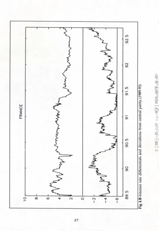
In this section we undertake an empirical analysis of the Spanish experience in the EMS target zone6. We would like to measure the effect of the existence of the EMS on the fundamentals; that implies, from an empirical point of view, to explore the relationship between (off-shore) interest rates differentials and the exchange rate deviations from the central parity, that is the relationship (6,s')- The solid lines in Figures 4.a,b show the interest rate differentials (6) and the dashed lines are exchange rate deviations from the central parity (s') of Spain with respect to the two countries object of our study: Germany and France.
The theoretical (6,s') curve has a negative slope. Further, we have seen that the relationship is non-linear for instantaneous rate differentials, becoming more linear and less steep as the maturity term increases (see Svensson (1991,b)); for our data set, with one month interest rate differentials, a linear relationship may be a good approximation which is easily formulated in practice, as in Weber (1991). Consequently, the expression equivalent to the basic model's postulate is the following:
8,-c,+fos,+er
Vr—c,-p ;
b<0
[13]
The intercept term, c„ under the original assumptions of the basic model (no realignment risk, no capital controls) is constant and equal to the drift of fundamentals (p), and the parameter b represents the response of the interest rate differentials to the exchange rate deviation from the central parity (s,'); the expected
6-The data are daily from 19/06/89 to 15/09/92 (788 observations), that is, from the entrance in the EMS to the first realignment of the Spanish peseta. Sources for the data are Servicio de Estadistica (Banco de Espana) and Datastream. Interest rates are Euromarkets one-month deposits.The central parities with respect to the German Mark and French Franc were set at 65 pts/DM and 19,38 pts/FF, respectively, and a 12% fluctuation band with respect to the central parity was allowed.
7 © The Author(s). European University Institute. version produced by the EUI Library in 2020. Available Open Access on Cadmus, European University Institute Research Repository.
value of b should be negative, since it conveys the honeymoon effect delivered by the target zone in the theoretical model.
Consider first the series 6, and s,' plotted in Figures 4; The scatterplots of both variables which appear under the title 'non-adjusted target zone' in Figures 5.A,B. (the observed (6,s,') curve) also display a rather diffuse relationship from where no definite relation between them can be observed. This would suggest that the empirical evidence does not support the basic model and this outcome confirms previous findings by Flood, Rose & Mathieson (1991), Weber (1991) among others, for other EMS countries, or Rodriguez (1992), for Spain. Exploring the reasons for the rejection of the basic model requires a statistical analysis of the series. The results of this analysis will also help us to reformulate the structure of the empirical model.
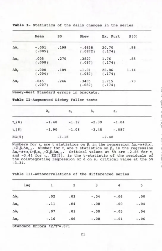
The summary statistics of the differenced series contained in Table 1 show several noteworthy points. Firstly, the series present an excess of kurtosis-mainly in the interest rate differentials- indicating that they are highly nonnormal; further, the column labeled S(0) provides estimates of the spectral densities at zero frequency. As noted by several authors, (e.g. Cochrane (1988)), this provides a useful diagnostic on the permanent (that is, components with a unit root) and transitory components in the series. Judging from point estimates, there seems to be far more persistence, in fact accentuation, of shocks in the interest rate differentials, than in the exchange rate deviations. On the contrary, the interest rate differentials could exhibit some degree of mean reversion towards a downwards trend, and this could lead to the rejection of a random walk model. Consequently, we test for the existence of a unit root in the autoregressive representation of each series against two alternatives: one consistent with fluctuations around a constant mean -r - , the other with stationary fluctuations around a deterministic linear trend-xT; Table II contains the corresponding Augmented Dickey-Fuller tests; In both cases eight lags are included to account for serial correlation.
We can see that there is very little evidence against the unit root hypothesis if the considered alternative is stationarity around a constant mean. However, as noted above, a more relevant alternative to consider for the interest differentials would be stationary fluctuations around a deterministic linear trend. As the results
show, the French differentials (6F) could be stationary-write l(0)-around a
deterministic trend, whereas the German differentials (6C) contain a unit root-write 1(1). Nevertheless, the results of the ADF test for (6F), do not seem too robust, since by only changing the number of lags in the tests, one should reject stationarity; i.e the ADF(7) gives a result of -3.22. Furthermore, by observing the persistence measures reported in Table I under the label S(0), we see that for both interest rates
© The Author(s). European University Institute. version produced by the EUI Library in 2020. Available Open Access on Cadmus, European University Institute Research Repository.
differentials the measures are very close to 1, that is, the measure of a pure random walk and so in what follows we will treat them as 1(1) variables7. Finally, both exchange rate deviations (s'F,s'c) are 1(1).
From these results, a cointegration relationship could be possible, for the four series are 1(1), hence we test for it: EG(5) in Table II shows that both series are not cointegrated, and as a consequence maintaining a constant parameter for c would also imply a unit root in Et. This means that interest rate differentials and exchange rate deviations can shift apart without bound. This is what explains the blurred relationship between 6 and s, when a constant c, is assumed as displayed in Figures 5.D.E, and the reason why we formulate a flexible model for c, of the form:
c ,- n f .pc, , < 0(B)r|,
[14]
W ith p e [0,1] ; 0( B ) -1- e , f l - e2f i 2- . . . . £ ( n , ) -0| £ (t i* ) -o*
with all the roots of 0(B)=O lying on or outside the unit circle, where B is the backshift operator, such that BSct=x,.k. With this specification, the only restriction that
is imposed on the model in [13] is that e, follows a white noise process. Given this
specification, we just have to explore the actual process for c„ given our data set. The lack of cointegration between the series 6 and s' implies that p equals 1, such that c, is 1(1) for both countries. Note that the unit root previously contained in the residuals (when c, was constant) is now shifted to the variable parameter c,. The second element to determine is the order of 0(B); this is done with the help of the autocorrelations of the differenced series, displayed in Table 3. There, we can see that for s' an IMA(1,1) process is an acceptable representation, whereas the series 6 seem to be well represented by a pure random walk. Therefore, the MA polynomial for c, is the sum of a MA(1) and a white noise, and a model for c, consistent with the data would be given by an IMA(1,1)- as shown in the Appendix 1- plus a drift (p.c). The value of this drift will arise from the estimation below.
Estimation procedure
The aim of this section is to estimate the model with the time-varying parameter c, and the time invariant parameter b of model [13], in order to achieve the relationship postulated by the theory, by extracting the intercept term component from the interest rate differential series 6.
7In order to compute the persistence measures S(0), univariate ARMA(2,2) models on the first differences of the series have been estimated, from where we have computed the univariate MA expansion, and finally we have evaluated it at B =l. Notice that a pure random walk, has persistence 1, and a stationary series 0.
9 © The Author(s). European University Institute. version produced by the EUI Library in 2020. Available Open Access on Cadmus, European University Institute Research Repository.
Rewriting [13] in the so-called state space form we obtain the following expression V Z .a .+ e . E (e,)-0 E(e*)-a^; where ' V - 6 l hs\ with Z-\1 0 0 0]; a and “,-for 1 ' 1 1 e o jO 1 o o " o o o o 0 0 1 0
E(ufit) - I A, the ider
where the unknown parameters b, fd, ar|2, a ,2, and 0 are chosen so that they satisfy the restrictions of Appendix 1, and maximize the likelihood function, or equivalently the log likelihood:
\ O Q L - h o Q 2 n - WC. ^r-1
[18]
where
er-6 ,-b s ,-Z at/t_,
The first equation is known as the measurement equation, and the second as the transition equation. Notice that the unobserved component c, and the drift for its process (p.c) are included in the state vector a t.
Having casted the model in State-Space, the Kalman Filter (KF) is a well- known method to compute the Gaussian likelihood function for a trial set of parameters (for a discussion see, for instance, Harvey (1989)). The filter recursively produces minimun mean square error (MMSE) estimates of the unobserved state vector given observations on Wt. The filter consists of two sets of equations, the
prediction and the updating or correction equations. Denoting the optimal
estimator of a,., based on information up to and including *PM, and letting P,_, denote
E(«,)-0, E(u(u(> 7 4 [15] ,-1g f, V i l ' [16] 1i v2i v3iJ o„ 0 0 0 0 0 0 0 ; R' o„ 0 0 0 i 0 0 0 0
inn matix o f order4
[17] © The Author(s). European University Institute. version produced by the EUI Library in 2020. Available Open Access on Cadmus, European University Institute Research Repository.
[19] the 4x4 covariance matrix of the estimation error, that is:
P, ,-£ [(« ,.,-a, ,)(<*, r a, i)1
the KF consists on the recursive application of the following set of equations to extract a value for the state a t:
Prediction Equations
a - Ta I20!
U t / t 1 i Mf l
V , - ” V , r +RQ/r
Parameter correction equations
ZA/I , F . 7 P 7 ' r t ^ r t / t< 7 'p -* tit-i-*' /r / ► a2 ar a,n -,,K ,e, P - P - K 7 P 1 i 1 i/t-i ■lNz'r i/i-i
where the subscript t/t-1 indicates that the optimal estimators for P and a are at time
t are computed with the information available at time t-1. Given initial values a,, P„
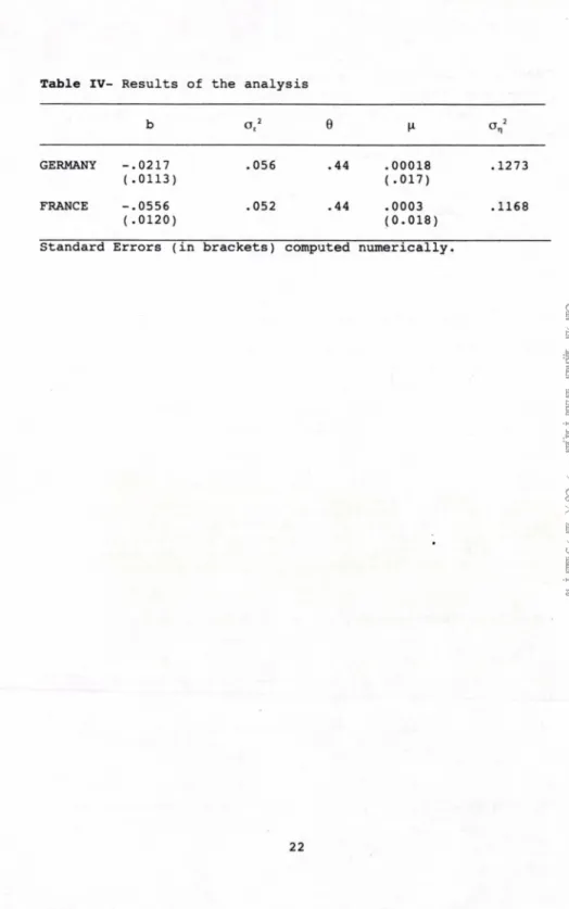
the filter computes the estimate at for a, at time t={l,2....,T}. In order to compute these initial values several alternatives are offered in the literature, as for instance the one devised by de Jong (1988) (see Appendix 2), which has been the one used here. Maximization of the log likelihood of the above state space model gives the results summarized in Table 4.
Figure 5,C shows the intercept terms c, for Germany and France and the right plot of figures 5,A,B display the adjusted interest rate differentials (6adi) obtained by substracting c, from 6„ that is, with the differentials net of the intercept term. Two results are worth underlining: Firstly, the sign of the response parameter b is negative, as the theory states, though its value is very small-see the slope of the
(bai’,s') scatterplot-, highlighting the scarce influence of the band on the interest rate
differentials (For France the band would explain 6,15% of the differentials; for Germany only 1,42%). Secondly, and as a consequence of the previous result, the term c, accounts for most of the differentials (the residuals (et) are white noise and of small magnitude-see Fig.5.D). Next we turn to the interpretation of these results.
Ill-Exploring the intercept: credibility
The disappointing results of the target zone model are partially explained by the behaviour of the series: the effect of the band on 6 relies on the expectation that
11 © The Author(s). European University Institute. version produced by the EUI Library in 2020. Available Open Access on Cadmus, European University Institute Research Repository.
the exchange rate will appreciate when it approaches the upper band, and viceversa; this suggest that the exchange rate is expected to revert to the interior of the band. However, the non-stationarity of s' indicates that the exchange rate does not display such mean reversion; thus, the position of the currency in the band cannot greatly influence the interest rate differentials8.
Another comment can further justify our results. Recall that in the empirical model we use deviations from the central parity-multiplied by a parameter to estimate b- (fas'), as an approximation to the exchange rate expectation within the band. On the other hand, since we are using Euromarket rates, it is reasonable to accept the fulfilment of the UCP. Then, if realignment risks are dismissed, the absence of a cointegrating relationship between s' and 6 would imply that the uncovered differentials contain a unit root. Accordingly,what c, picks up is precisely the realignment risk underlying the agents' expectations (c,=g,) and hence, bs' turns out to be a very poor approximation to the overall exchange rate expectation. The behaviour of c, very close to 5, shows that the interest rate differentials have reflected this implicit realignment risk, rather than the expectations derived from the position of the currency in the band.
The obvious conclusion to obtain from this analysis is that the band has not been completely credible during the sample under study. However, the decreasing profile of c, points out that the zone has gained credibility throughout the period, but for the last months, just before the effective realignment-as if anticipating it.
Although the unobserved components approach applied here is a credibility test in itself, we would like to assess the question of credibility on a more robust basis, applying to our data set the test devised by Svensson (1993) in which an explicit expected rate of realignment is estimated9.
This test is easily formulated from [11] and interpreting#, as the expected rate of realignment. Note that we only have to compute the expectation on the exchange rate conditional on no realignment; since the interest rates in the data set have a maturity of one month (= 20 observations) the regression to estimate is the following:
'-We should be cautious at this stage, since the lack of mean reversion can also be influenced by the wide band in which the peseta is allowed to fluctuate. For instance, Svensson (1993) rejects that s' are 1(1) for all the EMS original currencies, but the Italian Lira, that is, the generally acknowledged less reputed currency in the EMS, but also the only one fluctuating within a wide band.
9-An alternative test, also conceived by Svensson (1991,a), and applied to the Spanish peseta by Rodriguez (1992) and Ayuso et al. (1993) gives sufficient but no necessary conditions for rejecting that the band is credible, since it only accepts that the realignment takes place when the exchange rate reaches the limits of fluctuation.
© The Author(s). European University Institute. version produced by the EUI Library in 2020. Available Open Access on Cadmus, European University Institute Research Repository.
( L r t* h g r tm r v )~ ^ S l , l - 2 o ” m o + m i S |t l U l [22]
Taking expectations and substracting them from the interest rate differentials, an expected rate of realignment would be obtained. Comparing this result with [10], we can observe that this expected rate of realignment is an alternative way to estimate g,-the realignment risk. Note, however, that the previous integrability analysis prevents us from carrying out this regression, since the exchange rate is 1(1), and consequently the parameter m, is not significatively different from zero10. This means that, under this approach the expectation on the exchange rate conditional on no realignment is zero, and consequently, the expected rate of realignment is simply the interest rate differential.
This peculiar result reinforces rather than weakens our previous comments: as a matter of fact, it is no wonder that comparing the outcome of the Svensson test with the interpretation of c, as a realignment risk, we obtain very similar estimates of gr The reason is that underlying both approaches is the assumption that the expected exchange rate depreciation within the band is given by the position of the exchange rate in it. As we have seen, the data are not supportive of this hypothesis and that is why the estimated realignment risk virtually matches the interest rate differentials.
Despite the apparent robustness of this result we have to be extremely cautious to interpret the whole interest rate differential as a realignment risk. As Ayuso et al. (1993) point out, the expected realignment rate -or in its case c, -picks up expected exchange rate regime shifts, and this change in the implicit regime can actually occur while keeping the same central parity (for instance, a jump from the lower to the upper part of the same band). This implies that the interest rate differentials would overestimate the realignment risk; note that this possibility is even more likely in the case of a wide band.
Conclusions and final remarks
The results of the Kalman Filter -implemented to explore the importance of the band in the behaviour of the interest rate differentials- have been interpreted in the previous section. The main conclusion is that we do not find enough empirical evidence to support the target zone hypothesis for Spain. We have seen that the
'“-The estimation of As'„2„ instead of As',,,- as in the integrability analysis- does not have any implication for the value of m,. Further, Lopez (1993), using the asymptotic distributions of the DF statistic, shows that the standard Dickey-Fuller critical values have to be multiplied by a correction factor of 1.22, when the number of lags used is larger than 5; this implies that the rejection region is larger.
13 © The Author(s). European University Institute. version produced by the EUI Library in 2020. Available Open Access on Cadmus, European University Institute Research Repository.
target zone has hardly influenced the interest rate differentials of Spain respect to Germany and France and these interest rate differentials have largely reflected risks of realignment (or risks of effective regime shifts); the parameter c,, which contains a unit root, conveys this risk and basically explains the differentials. However, the evolution of c„ along with other factors which caracterize the period under consideration (reduction of interest differentials, strength of the peseta in the band, growth of the Spanish stock of reserves), demand some additional comments.
First of all, recall from [9] that the realignment risk can be decomposed into two components: the expected size of realignment and the probability attached to it
(p). One can accept taht the magnitude of the realignment depends on the
expectations that agents assign to the evolution of the fundamentals, on their actual evolution and on the difference between these two; this component should behave smoothly in absence of news. On the contrary, the second component-the probability attached by the agents to a realignment- can be highly volatile, and a jump in p can trigger a self-sustained process resulting in a proper speculative attack.
Secondly, the variability showed by c, and, especially, its progressive reduction until mid-1992 reveal the existence of several elements determine its evolution. On the one hand, nominal convergence is reflected in the reduction of the interest differentials and, consequently, of the realignment risk; on the other hand, the process of financial integration implemented during this period, in conjunction with sterilized interventions (announcement effect) may have allowed meaningful gains in the credibility of the exchange rate commitment; these gains have been reflected in the lower probability of the current band being abandoned-at least in the short run- and, consequently, in a lower realignment risk.
Finally, these factors which allow for the reduction in c, appear to vanish around the end of the period (Summer '92): the deviations of the fundamentals from the policy targets, the general instability in the EMS and the uncertainties of the Monetary Union (elements which can be seen as positive shocks on p) swiftly erode the previous credibility gains and the term c, displays a change of trend; in terms of the above interpretation, the probability of a realignment which bridges the gap in the fundamentals, begin to increase. This increase in the realignment risk cannot be stopped either by the increase in the interest rate differentials nor by the depreciation of the currency within the band nor by the massive sell of reserves, and results in the strong speculative pressures which ended up causing the first realignment of the Spanish peseta on 16, September 1993.
© The Author(s). European University Institute. version produced by the EUI Library in 2020. Available Open Access on Cadmus, European University Institute Research Repository.
Appendix 1 Consider the model:
6 , - c + b s + c ,
where 6, and s', are observable but c, and e, are not. For simplicity and without loss of generality the drifts have been set equal to zero. If one of them is different from zero the resulting model for c, will contain also a drift equal to that. If both 6, and s', have drift, the resulting drift will be that of 6 minus that of s'
Assume also that e, is a white noise process serially and contemporaneously
uncorrelated with c„ and s',. Assume also that the process for 6, and s', are known to be:
A6 r-»r,; As>v,- Yvm
a 2iv, o 2. known
applying first differences in the original model we therefore obtain: A f > - A c - b A s ' * A t ' ,
substituting
M'>”Ae,+Ai,,-frYri,-1*Ae ^ equivalently
A c r wr bv+b r r \, _, - At ,
Notice that the right hand side (r.h.s) of the above equation is the sum of a white noise process and two MA(1) processes, one of them with a unit root, and in consequence the r.h.s will itself be a MA(1), given say, by (l-0B)r)„ with E(q)=0 and E(r)2)=on2. These last parameters have to satisfy the constraints implied by equating the autocovariances of the l.h.s. and r.h.s. of the above equation. The variance and first autocovariance yield the system:
(1 +02) o 2 - o 2n+b2o 2.+b2y2o^.+2of -0o„ - b y o v- a t• 2 * * 15 © The Author(s). European University Institute. version produced by the EUI Library in 2020. Available Open Access on Cadmus, European University Institute Research Repository.
and for further lags equal to zero.
Assume now that b is known, and denote:
x: - a 2n+bza 2v( 1 +v2)
u2 2
x2- b yo,
with all the terms in x, and x2 known.
However, the system is underidentified, since we have two equation with three unknowns. In fact the most we can do is to solve the system for two of the unknowns in terms of the third one. Choosing at2 as the latter and solving for the former we get:
1
chosing 0, such that I0I<1
with
, _ - V 2tU 2 x2+ot
also
It is also immediate to prove that 2s j z | and since 0,02=1, one of the 0s is
always in absolute value less or equal to 1. Finally since crt2 is not known, it is chosen so that that the log likelihood is maximized.
Appendix 2
In principle the starting values for the KF a0 and P0, are given by the mean and the covariance matrix of the unconditional distribution of the state vector. However when the state equation is nonstationary the unconditional distribution of the state vector is not defined. Unless genuine prior information is available, the initial
distribution of a 0 must be specified in terms of a diffuse prior. If we write P0=kI,
where k is a positive scalar, the diffuse prior is obtained as k->°o. This corresponds
with Po’=0. The distribution is an improper one since it does not integrate to one.
However, as Gomez and Maravall (1993) note, the use of the so called big k method
is not only numerically dangerous but also inexact. Alternative initialization
procedures can be found in de Jong (1988) (the one used), Carraro & Sartore (1987) and Gomez & Maravall (1993). In de Jong's algorithm it is assummed that the initial state vector can be partitioned into D nonstationary and N-D stationary elements, and expressed as: © The Author(s). European University Institute. version produced by the EUI Library in 2020. Available Open Access on Cadmus, European University Institute Research Repository.
“i=C,y,+C2y2
where Yi is a Dxl vector containing the D non stationary elements, with a diffuse
prior, that is Var(Y,)='»I or [Var(Y,)]'’=0, while an N-Dxl vector has a proper
prior, that is,
E(Y2)=m Var(Y2)=V
In our model with stationary errors m is a 3X1 where the first element is set equal to a consistent estimate of /i and the two other elements are zero, while V is diagonal matrix with zero the first element of the diagonal os as given in Appendix
1; Yi would be set equal to c, while y2=[m hi ht-i]’; C,=[l 0 0 0]' and C: =[0 I,]'. The use
of the big k approximation for y, is avoided by extending the KF as follows. Define
Xt=[<Pt 0]
where 0 in [.] is a null matrix with D columns, (so in the model D=l). Then the standard KF recursions would be initiated with
P°,io=C2V C 2'
The recursion for the state vector is augmented so as to become a recursion for the
matrices A, and At| defined as:
At=At|w+P V 1Z'Ft,Nl t= l T where Nt=X,-ZAt|„ At|i.i=TA,., with A, |0=[C2m C,] and St=St.,+NtF,-'Nt t= l T with S„=0
The output from the above recursions is used to construct the required statistics from the diffuse prior model as follows. First, partition N„ A, and St as follows:
N,=[vt° N*t], A,=[at° A4,] and S,=[Stt S2t]' with
S„=[S4t° s\'] S21=[s*t S*J
Then as shown by de Jong (1989), the estimator of the vector for the diffuse prior starting values is:
17 © The Author(s). European University Institute. version produced by the EUI Library in 2020. Available Open Access on Cadmus, European University Institute Research Repository.
a.=At[l -s*t'S*t-]'; and
P,=P\°A\S\-A\’
where S*,‘ is the generalized inverse of S*r
The log likelihood function, ignoring the constant term, is given by
£,=-*41In | F, | -V&'°-Y&n | s*T | +V4s*T'S V ,s*T
The expression for the log likelihood assumes that the KF recursions are carried on until the end of the sample. However once S\ becomes nonsingular the diffuse filter can be collapsed to the usual filter. If S*t is nonsingular at some point t=x, then the usual KF can be employed starting from values obtained for a, and P, for t=x.
It can be shown that S+, is non singular if r[C,'Z', C I'T'Z',C1'T'T,Z',..../C,T'...Z']=D
Since in our particular case r(C ,'Z')=l, we can truncate at x=l, and the log likelihood function for the T observations becomes
£=£,-142In | F, | -*42et'Ft 'et
with £, defined as above and the sums evaluated only at t=l.
B IB L IO G R A P H Y
ALBEROLA,E. J.H.LOPEZ, V.ORTS (1993)."Target zone models in a context of financial integration. An empirical analysis of the Spanish experience in the EMS". Annali d'Economia della Università di Trento.
AYUSOJ. M.PEREZ, F.RESTOY (1993). "Indicadores de credibilidad de un régimen cambiario: el caso de la peseta en el SME". Banco de Espana, manuscript.
ARTIS,M. and M.P. TAYLOR (1988)."The EMS: Assessing the track record",in "The EMS". Giavazzi,F, Mirassi,S. Miller,M eds,cap.7, CUP.
BERTOLA,G. and L. SVENSSON (1993)."Stochastic devaluation risk and the empirical fit of target-zones models", Review of Economic Studies, forthcoming.
CARRARO,C. and D. SARTORE (1987)."Square Root Iterative Filter: Theory and Applications to Econometric Models", Annales D'Economie et Statistique N 6/7
© The Author(s). European University Institute. version produced by the EUI Library in 2020. Available Open Access on Cadmus, European University Institute Research Repository.
COCHRANEJ.H. (1988). "How big is the random walk in the GNP?", Journal of Political Economy, 96.
DE JONG, P. (1988). "The likelihood for a state space model", Biometrika,75. DOMINGUEZ,K. and J. FRANKEL (1990)."Does foreign exchange intervention matter?. Disentangling the portfolio and expectations effects for the mark". NBER, 3299.
FLOOD,R., D. MATHIESON and A. ROSE (1991)."An empirical exploration of exchange rate target-zones", Carnegie-Rochester series on Public Policy, 35.
FRANKEL,J.A. and S. PHILLIPS (1991)."The EMS: credible at last?". NBER Working paper n.3891
FRENKEL,J.A. and A.T. MacARTHUR (1988)."Political vs. currency premia in international real interest rates differentials",European Economic Review,32 GIAVAZZ1,F. and A. GIOVANNINI (1989).Limiting exchange rate flexibility,MIT press.
GIAVAZZLF., S. MICOSSI and M. MILLER (1988)."The European Monetary System",CUP
GIAVAZZLF. and M. PAGANO (1988)."The advantage of tying one's
hands".European Economy,32.
GOMEZ, V., A.MARAVALL (1993),"Initializing the Kalman filter with incompletely specified initial conditions", EU1 Working Paper, 93/7.
HARVEY,A.C. (1989). Forecasting structural time series models and the Kalman filter. Cambridge University Press.
KRUGMAN.P. (1990)."Target zones and exchange rate dynamics", Quarterly Journal of Economics, 106
KRUGMAN,P. and J. ROTEMBERG (1990)."Target zones with limited
reserves",Mimeo,July '90
LOPEZ,J.H. (1993)."Testing for unit roots with the k-th autocorrelation coefficient”, Mimeo, EUI.
MASTROPASQUA,C. MICOSSI,S. RINALDI,R. (1988)."Interventions, sterilization and monetary policy in EMS countries, 1979-87" in "The EMS". Giavazzi,F, Micossi,S. Miller,M eds,ch,10, CUP.
NEWEY,W.K. WEST,K. (1987)."A simple positive semidefinite, heteroskedaticity and autocorrelation consistent covariance matrix", Econometrica,55.
19 © The Author(s). European University Institute. version produced by the EUI Library in 2020. Available Open Access on Cadmus, European University Institute Research Repository.
OBSTFELD,M. (1988)."The effectiveness of foreign-exchange intervention: recent experience". NBER Working Paper No.2796.
RODRIGUEZ, H. (1992). "Contrastes de credibilidad para la banda de fluctuation de la peseta en el SME". Moneda y Credito, 195.
ROGOFF,K. (1985). "Can exchange rate predictability be achieved without monetary convergence?.European Economic Review,28
SVENSSON,L. (1989)."Target zones and interest rate variability", CEPR Discussion Paper, n.372
SVENSSON,L. (1991,a)."The simplest test of target zone credibility”,IMF Staff Papers, n.38.
SVENSSON,L. (1991,c)."The term structure of interest rate differentials in a target zone". Journal of Monetary Economics,28.
SVENSSON,L. (1993). "Assessing target zone credibility: mean reversion and devaluation expectations in the EMS", European Economic Review, 37.
WEBER,A.A. (1991).”Time-varying devaluation risk, interest rate differentials and exchange rates in target zones: evidence from EMS",CEPR Workshop on exchange rates,Oct '91. © The Author(s). European University Institute. version produced by the EUI Library in 2020. Available Open Access on Cadmus, European University Institute Research Repository.
Table I- Statistics of the daily changes in the series
Mean SD Skew E x . Kurt S(0)
a ô g -.001 (.005) . 199 -.4638 20.70 (.0872) (.174) .98 As g .005 (.008) .270 .3827 1.76 (.087) (.174) .85 Aó f -.000 ( .004 ) .189 -1.01 20.86 (.087) (.174) 1.14 As f .045 (.007) .246 .3405 1.715 (.087) (.174) .73
Newey--West Standard errors in brackets.
Table II-Augmented Dickey Fuller tests
6c sG S F
t m(8) - 1 . 48 1.12 -2.39 -1.04
i,(8) - 1 . 90 1.08 -3.48 -.087
EG(5) -1.18 -2.48
Numbers for xv are t statistics on p„ in the regression Axt=«+poxt_
^SjPjAXj.j. Number for t, are t statistics on po in the regression
Axt= a + a 1t+P0xt_1+2jPjAxt_:j. Critical values at 5% are -2.86 for xM
and -3.41 for t,. EG(5), is the t-statistic of the residuals of the cointegrating regression of 6 on s, critical value at the 5% -3.34.
Table Ill-Autocorrelations of the differenced series
lag 1 2 3 4 5 Aôg .02 o ro -.04 -.06 .00 As g -.11 .04 -.08 .00 -.04 Aò f .07 .01 -.00 -.05 .04 As f -.16 .06 -.08 -.01 -.06 Standard Errors ±2/Tl’=.071 21 © The Author(s). European University Institute. version produced by the EUI Library in 2020. Available Open Access on Cadmus, European University Institute Research Repository.
Table IV- Results of the analysis b a , 2 e < GERMANY -.0217 .056 .44 .00018 .1273 (.0113) (.017) FRANCE -.0556 .052 .44 .0003 .1168 (.0120) (0.018)
Standard Errors (in brackets) computed numerically.
© The Author(s). European University Institute. version produced by the EUI Library in 2020. Available Open Access on Cadmus, European University Institute Research Repository.
23 EX CH ANG E R A TE DEV IATIONS FU NDA ME NT AL DEV IATIONS F ig .l -R e la ti o n b et w ee n e xc h a n g e rates, fu nd a m ent al s an d i nt ere st rates. Th e p a ra m ete rs a re p = 2, a = 0 .1 . D as he d line d isp la y s the d ri ftl es s case; so li d li ne in cl u de s a dri ft in th e fu nd a m ent a ls (# i= 2% ) © The Author(s). European University Institute. version produced by the EUI Library in 2020. Available Open Access on Cadmus, European University Institute Research Repository.
g-2 -C o n sta n t d ev a lu a ti o n ri sk : exp ec te d siz e is 6 % and pro ba b ili ty is 0, 5. T h e cu rv e is s hi fte d to th e le ft. © The Author(s). European University Institute. version produced by the EUI Library in 2020. Available Open Access on Cadmus, European University Institute Research Repository.
|0;iu9J9jj!p ajo j }S9J9;u! <D O <U G1 C o n u X <u 2 5 Fi g. 3 -C o n sta n t d ev a lu a ti o n ri sk and int ere st rate d if fe re nt ia ls . © The Author(s). European University Institute. version produced by the EUI Library in 2020. Available Open Access on Cadmus, European University Institute Research Repository.
O O O C O M - C N O C N ^ l D ^ I l l
in
CM CD CM CD in CD CD m o CDo
CDin
CD CO F ig .4 .A .-In te re st ra te d if fe re n tia ls a n d d ev ia tio n s from the ce nt ra l par it y . (198 9-93 ) © The Author(s). European University Institute. version produced by the EUI Library in 2020. Available Open Access on Cadmus, European University Institute Research Repository.2 7 F ig 4 .B -I n te re st rate d if fe re n tia ls and d ev ia tio n s from ce ntr al p a ri ty .(19 8 9 -9 3 ) © The Author(s). European University Institute. version produced by the EUI Library in 2020. Available Open Access on Cadmus, European University Institute Research Repository.
I lT> LD I F ig .5 .A -I n te re st d if fe re n tia ls (st and ard and ad ju st ed ) and d ev ia tio n s from the ce ntr al par it y . S ca tte rp lo t. © The Author(s). European University Institute. version produced by the EUI Library in 2020. Available Open Access on Cadmus, European University Institute Research Repository.
I F ig .5 .B .-In te re st rate d if fe re n tia ls (st and ard a n d ad ju st ed ) an d d ev ia tio n s from the ce nt ra l par it y . S ca tte rp lo t. © The Author(s). European University Institute. version produced by the EUI Library in 2020. Available Open Access on Cadmus, European University Institute Research Repository.
F ig .5 .D .-R es id u a ls o f th e mo del . © The Author(s). European University Institute. version produced by the EUI Library in 2020. Available Open Access on Cadmus, European University Institute Research Repository.
3 1 F ig .5 .C -I n te rc e p t term ( c^ ) © The Author(s). European University Institute. version produced by the EUI Library in 2020. Available Open Access on Cadmus, European University Institute Research Repository.
© The Author(s). European University Institute. version produced by the EUI Library in 2020. Available Open Access on Cadmus, European University Institute Research Repository.
EUI
WORKING
PAPERS
EUI Working Papers are published and distributed by the European University Institute, Florence
Copies can be obtained free of charge - depending on the availability o f stocks - from:
The Publications Officer European University Institute
Badia Fiesolana
1-50016 San Domenico di Fiesole (FI) Italy
Please use order form overleaf
© The Author(s). European University Institute. version produced by the EUI Library in 2020. Available Open Access on Cadmus, European University Institute Research Repository.
Publications of the European University Institute
To The Publications Officer
European University Institute Badia Fiesolana
1-50016 San Domenico di Fiesole (FI) - Italy Telefax No: +39/55/573728 From N am e. . Address. i : i
□ Please send me a complete list of EUI Working Papers □ Please send me a complete list of EUI book publications □ Please send me the EUI brochure Academic Year 1994/95 □ Please send me the EUI Research Review
Please send me the following EUI Working Paper(s):
No, Author ... T itle: ... No, Author ... Title: ... No, Author ... T itle: ... No, Author ... T itle: ... Date ... Signature ... © The Author(s). European University Institute. version produced by the EUI Library in 2020. Available Open Access on Cadmus, European University Institute Research Repository.
Working Papers of the Department of Economics Published since 1990
ECO No. 90/1
Tamer BASAR and Mark SALMON Credibility and the Value of Information Transmission in a Model of Monetary Policy and Inflation
ECO No. 90/2 Horst UNGERER
The EMS - The First Ten Years Policies - Developments - Evolution ECO No. 90/3
Peter J. HAMMOND
Interpersonal Comparisons of Utility: Why and how they are and should be made
ECO No. 90/4 Peter J. HAMMOND
A Revelation Principle for (Boundedly) Bayesian Rationalizable Strategies ECO No. 90/5
Peter J. HAMMOND
Independence of Irrelevant Interpersonal Comparisons
ECO No. 90/6 Hal R. VAR1AN
A Solution to the Problem of Externalities and Public Goods when Agents are Well-Informed
ECO No. 90/7 Hal R. VARIAN
Sequential Provision of Public Goods ECO No. 90/8
T. BRIANZA, L. PHLIPS and J.F. RICHARD
Futures Markets, Speculation and Monopoly Pricing
ECO No. 90/9
Anthony B. ATKINSON/ John MICKLEWRIGHT
Unemployment Compensation and Labour Market Transition: A Cridcal Review
ECO No. 90/10 Peter J. HAMMOND
The Role of Information in Economics
ECO No. 90/11
Nicos M. CHRISTODOULAKIS Debt Dynamics in a Small Open Economy
ECO No. 90/12 Stephen C. SMITH
On the Economic Rationale for Codetermination Law ECO No. 90/13 Elettra AGLIARDI
Learning by Doing and Market Structures ECO No. 90/14
Peter J. HAMMOND Intertemporal Objectives ECO No. 90/15
Andrew EVANS/Stephen MARTIN Socially Acceptable Distortion of Competition: EC Policy on State Aid ECO No. 90/16
Stephen MARTIN
Fringe Size and Cartel Stability ECO No. 90/17
John MICKLEWRIGHT
Why Do Less Than a Quarter of the Unemployed in Britain Receive Unemployment Insurance? ECO No. 90/18 Mrudula A. PATEL
Optimal Life Cycle Saving With Borrowing Constraints: A Graphical Solution ECO No. 90/19 Peter J. HAMMOND
Money Metric Measures of Individual and Social Welfare Allowing for Environmental Externalities ECO No. 90/20 Louis PHLIPS/ Ronald M. HARSTAD
Oligopolistic Manipulation of Spot Markets and the Timing of Futures Market Speculation © The Author(s). European University Institute. version produced by the EUI Library in 2020. Available Open Access on Cadmus, European University Institute Research Repository.
ECO No. 90/21 Christian DUSTMANN
Earnings Adjustment of Temporary Migrants
ECO No. 90/22 John MICKLEWRIGHT The Reform of Unemployment Compensation:
Choices for East and West ECO No. 90/23 Joerg MAYER
U. S. Dollar and Deutschmark as Reserve Assets
ECO No. 90/24 Sheila MARNIE
Labour Market Reform in the USSR: Fact or Fiction?
ECO No. 90/25 Peter JENSEN/
Niels WESTERGARD-NIELSEN Temporary Layoffs and the Duration of Unemployment: An Empirical Analysis ECO No. 90/26
Stephan L. KALB
Market-Led Approaches to European Monetary Union in the Light of a Legal Restrictions Theory of Money ECO No. 90/27
Robert J. WALDMANN
Implausible Results or Implausible Data? Anomalies in the Construction of Value Added Data and Implications for Esti mates of Price-Cost Markups ECO No. 90/28 Stephen MARTIN
Periodic Model Changes in Oligopoly ECO No. 90/29
Nicos CHRISTODOULAKIS/ Martin WEALE
Imperfect Competition in an Open Economy
ECO No. 91/30
Steve ALPERN/Dennis J. SNOWER Unemployment Through ‘Learning From Experience’
ECO No. 91/31
David M. PRESCOTT/Thanasis STENGOS
Testing for Forecastible Nonlinear Dependence in Weekly Gold Rates of Return
ECO No. 91/32 Peter J. HAMMOND Harsanyi’s Utilitarian Theorem: A Simpler Proof and Some Ethical Connotations
ECO No. 91/33 Anthony B. ATKINSON/ John MICKLEWRIGHT
Economic Transformation in Eastern Europe and the Distribution of Income* ECO No. 91/34
Svend ALBAEK
On Nash and Stackelberg Equilibria when Costs are Private Information ECO No. 91/35
Stephen MARTIN
Private and Social Incentives to Form R & D Joint Ventures ECO No. 91/36
Louis PHLIPS
Manipulation of Crude Oil Futures ECO No. 91/37
Xavier CALSAMIGLLA/Alan KIRMAN A Unique Informationally Efficient and Decentralized Mechanism With Fair Outcomes
ECO No. 91/38
George S. ALOGOSKOUFIS/ Thanasis STENGOS
Testing for Nonlinear Dynamics in Historical Unemployment Series ECO No. 91/39
Peter J. HAMMOND
The Moral Status of Profits and Other Rewards:
A Perspective From Modem Welfare
© The Author(s). European University Institute. version produced by the EUI Library in 2020. Available Open Access on Cadmus, European University Institute Research Repository.