Advanced gamma-ray spectrometry
for environmental radioactivity monitoring
by
Gerti Xhixha
Submitted to
The University of Ferrara
(Faculty of Mathematics, Physics and Natural Sciences)
for the degree of
PhD in Physics
March 2012
Table of content
Chapter 1
... 22
Introduction to environmental radioactivity: from cosmos to man-made ... 22
1.1 Cosmic radiation and cosmic-ray produced radionuclides ... 22
1.2 Primordial radionuclides ... 24
1.2.1 Potassium, uranium and thorium ... 26
1.2.2 Radioactive decay series ... 31
1.3 Man-made radionuclides ... 34
Chapter 2
... 39
Laboratory ray spectrometry: a fully automated low-background high-resolution
γ-ray spectrometer ... 39
2.1 MCA_Rad system: set-up design and automation ... 39
2.1.1 Features of HPGe detectors ... 39
2.1.2 Shielding design and evaluation ... 41
2.1.3 Automation: hardware and software developments ... 45
2.2 MCA_Rad system calibration ... 47
2.2.1 Energy calibration ... 47
2.2.2 Efficiency calibration with uncertainty budged ... 48
2.3 Case of study: bedrock radioelement mapping of Tuscany Region, Italy ... 60
2.3.1 Representative sampling and sample preparation strategy for bedrock radioelement
mapping ... 66
2.3.2 Summary of the results: bedrock radioelement mapping ... 68
2.4 Appendix A: calculation of simplified coincidence summing correction factor for
152Eu
... 75
Chapter 3
... 80
In-situ γ-ray spectrometry: an alternative method on calibration and spectrum analysis
... 80
3.1 In-situ gamma-ray spectrometry using portable NaI(Tl) scintillation detectors ... 80
3.1.1 ZaNaI system set-up and calibration procedure ... 80
3.1.2 An alternative approach for calibration and spectrum analysis ... 85
3.2.1 Brief geological settings: Ombrone Valley (Tuscany Region) ... 93
3.2.2 In-situ measurements: summary of the results ... 95
3.3 Study of correlation between in-situ and laboratory measurements ... 98
Chapter 4
... 105
Airborne γ-ray spectrometry: a geostatistical interpolation method based on geological
constrain for radioelement mapping ... 105
4.1 A self-made airborne gamma-ray spectrometer ... 105
4.1.1 AGRS system: set-up ... 105
4.1.2 Calibration and radiometric data processing ... 107
4.2 The first airbone gamma-ray spectrometry survey in Italy: case of study Elba island 112
4.2.1 Brief geological setting ... 112
4.2.2 Airborne survey: summary of the results ... 115
4.3 Radioelement mapping using geostatistical methods ... 118
Chapter 5
... 134
Conclusions ... 134
List of figures and tables
Chapter 1
Figure 1.1: simplified schematic representation of a hadronic shower originated by a high-energy proton. Figure 1.2: potassium decay modes.
Figure 1.3: uranium decay chain. Fig. 1.4: thorium decay chain.
Figure 1.5: secular equilibrium buildup of a very short-lived daughter (222Rn of half-life 3.824 d) from a long-lived parent (226Ra of half-life 1600 y). The activity (arbitrary unit) of the parent remains constant, while the activity of the daughter reaches secular equilibrium (more than 99%) just after seven half-lives.
Figure 1.6: transient equilibrium of the decay of 234U (of half-life 2.45 x 10⁵ y) to 230Th (of half-life 7.54 x 10⁴ y). The activity ratio daughter/parent approaches the constant value 1.48.
Figure 1.7: no equilibrium: the growth and decay of 90Rb (of half-life 158 s) from 90Kr (of half-life 33.33 s). If 90Kr is not continuously produced it will vanish more quickly producing 90Rb which on turn will vanish quickly respective 90Sr having a much longer half-life and reaching secular equilibrium with its daughter 90Y.
Figure 1.8: the global distribution of the locations of all nuclear tests and other detonations worldwide. Atmospheric tests are
in blue, underground tests in red. Successively larger symbols indicate yields from 0 to 150 kt, from 150 kt to 1 mt, and over 1 mt. Data taken from: http://www.johnstonsarchive.net/.
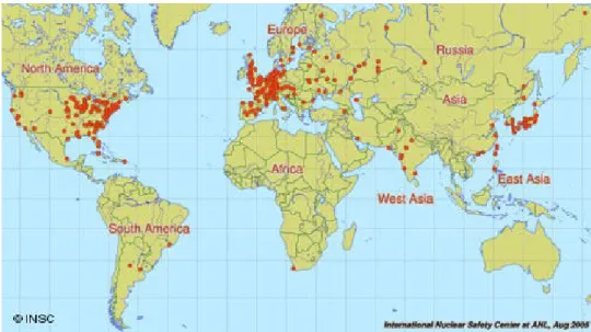
Figure 1.9: distribution of 440 nuclear power plants operating around the world.
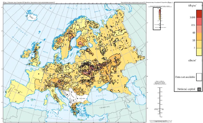
Figure 1.10: European map 1 : 11 250 000 of 137Cs deposition following Chernoby NPP accident. Data taken from: http://rem.jrc.ec.europa.eu/.
Table 1.1: confrontation of some models used for the estimation of cosmic radiation dose based on digital terrain model. Table 1.2: heads of decay chain segments in uranium decay chain and the respective grow-up times.
Table 1.3: heads of decay chain segments in thorium decay chain and the respective grow-up times.
Table 1.4: dose conversion coefficients for external gamma radiation coming from natural radionuclides present in soil. Table 1.5: principal radionuclides released (volatile elements) in Chernobyl accident compared to those assumed from
Chapter 2
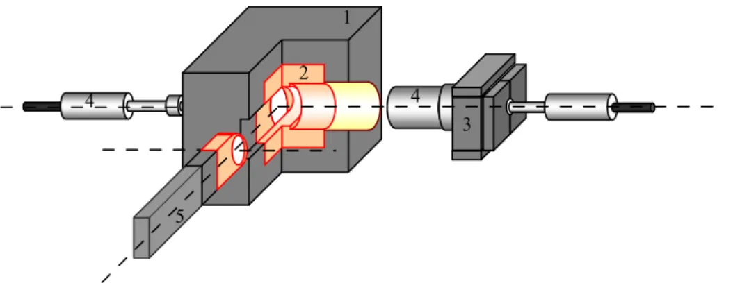
Figure 2.1a: schematic design of the MCA_Rad system. 1) The main lead shielding construction (20 cm x 25 cm x 20 cm).
2) The core copper shielding (10 cm x 15 cm x 10 cm). 3) The rear lead shielding construction. 4) HPGe semiconductor detectors. 5) The mechanical sample changer.
Figure 2.1b: view of MCA_Rad system.
Figure 2.2: the total attenuation coefficients of a standard graded shielding composition showing the migration of X-rays
toward low energy range. Data taken from National Institute of Standards and Technologies (NIST) (http://www.nist.gov) XCOM 3.1 Photon Cross Sections Database.
Figure 2.3: MCA_Rad system background spectra (live time 100h) without (red) and with (green) shielding showing a
reduction of two order of magnitudes.
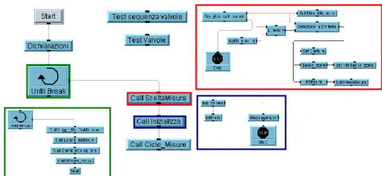
Figure 2.4: the VEE graphical algorithm which drive the MCA_Rad system. Figure 2.5: energy calibration function for the MCA_Rad system.
Figure 2.6: standard spectra of 152Eu, 56Co and background normalized for one hour.
Figure 2.7: simplified decay scheme showing the effect of summing in and out.
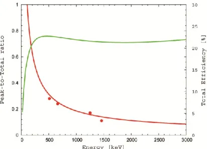
Figure 2.8: empirical calculation of P/T ratio curve (red) and experimental check by measuring single and double gamma ray
emitting points sources like 137Cs, 60Co, 40K and 22Na. The related total efficiency curve (green).
Figure 2.9: absolute efficiency curve for the MCA_Rad system obtained by fitting the corrected values for coincidence
summing with equation 2.16. Apparent efficiencies of 152Eu (blue triangles) and 56Co (green squares) are also presented.
Figure 2.10: measurement configuration of the experimental measurement done for the calculation of geometrical correction
factor.
Figure 2.11: curve reconstructing the geometrical correction factor obtained by fitting photopeaks of 56Co and 57Co with a third order polynomial (Eq. 2.19).
Figure 2.12: average mass attenuation coefficient deduced from weighting different rock forming minerals (calcite (CaCO3); quartz (SiO2); dolomite (CaMg(CO3)2); feldspar albite (NaAlSi3O8); feldspar anorthite (CaAl2Si2O8); feldspar orthoclase (KAlSi3O8); anhydrite (CaSO4); gypsum (CaSO4:2H2O); muscovite (KAl2(Si3)O10(OH,F)2); rutile (TiO2); bauxite gisbbsite (Al(OH)3).
Figure 2.13: the geological map of Tuscany at scale 1:250,000.
Figure 2.15: the spatial distribution of 882 samples (blue triangle soil and red circle rocks samples) collected over the
territory of Tuscany Region for the realization of potential natural radioactivity concentration of bedrocks.
Figure 2.16: the potential annual effective dose equivalent weighted for the Tuscany Region area and calculated based on the
characterisation of geological formational domains.
Figure 2.17: distribution of total activity (Bq/kg) in principal geological formations characterized with more than 10 samples.
The box plot encloses 50% of the values while the whiskers include other 45% of them. The data exceeding this limits are the outliers and extremes.
Figure 2.18: the distribution of potassium, uranium, thorium and the relative total activity concentration for 882 sample. Figure 2.19: the potential total activity concentration of bedrocks in Tuscany Region realized through the utilization of 882
sample.
Figure A-1: simplified decay scheme for 152Eu for gamma energies.
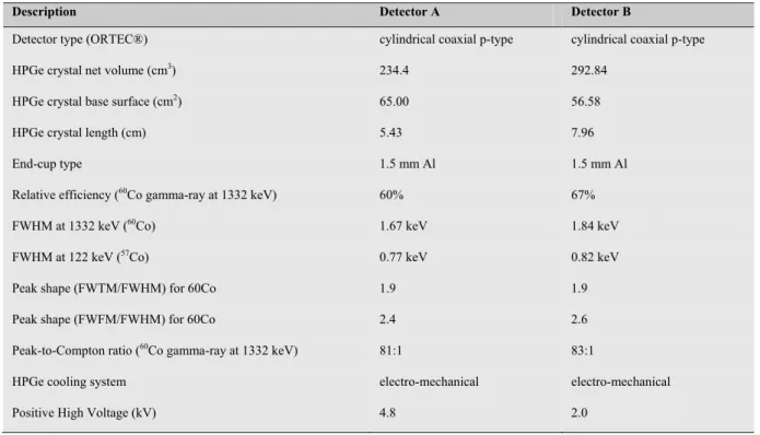
Table 2.1: the features of the two detectors used in the project design of MCA_Rad system.
Table 2.2: characterization of MCA_Rad system background (Bckg. without shielding and Bckg. with shielding) expressed
in count per hour (cph) for the most intense energetic lines and the corresponding detection limit LD in counts (Eq. 2.1) for 95% confidence interval (CI) and minimum detectable activity (MDA) in Bq/kg (Eq. 2.2).
Table 2.3: apparent efficiency and corrected efficiencies for coincidence summing according to equation 2.15.
Table 2.4: activity concentrations calculated for the main energetic lines used to study the 238U and 232Th decay chains and for 40K and the respective statistical uncertainty. An evaluation of efficiency calibration method uncertainty budged is described in details below.
Table 2.5: uncertainty budged evaluation for efficiency calibration method.
Table 2.6: typical statistical uncertainty for activity concentration ranges for 1h of acquisition time. The evaluation was done
for 609 keV (214Bi), 583 keV (208Tl) considering secular equilibrium and 1460 keV (40K).
Table 2.7: radioactivity characterization for 42 geological formation domains by MCA_Rad system for 1h acquisition time
(1σ is the standard deviation) with (*) is reported the median value.
Table A-1: tables of coincidence summing coefficients calculated and compared with bibliographic values.
Chapter 3
Figure 3.2: worldwide calibration facilities (pad): data source IAEA 2010. Figure 3.3: example of a natural calibration site (GC1 see table 3.3).
Figure 3.4: spectra acquired in-situ (black dashed line) compared with the fit (full red line) obtained by the FSA with NNLS
constrain (described later). The 137Cs contribution is shown alone (green dotted line) to underline the need to include this element in the analysis.
Figure 3.5: the spectra acquired in CA1 site in (red full line). The fit obtained using the concentrations measured with the
MCA_Rad system is also reported (black dashed line).
Figure 3.6: the sensitive spectra of 137Cs, obtained using the standard FSA method. The green line is placed to show the zero count level.
Figure 3.7: the sensitive spectra of 238U, obtained using the standard FSA method. The region where there are negative counts is emphasized in the box.
Figure 3.8: the sensitive spectra obtained through the FSA method with NNLS constrain.
Figure 3.9: the geological map 1:50,000 of Ombrone basin showing the distribution of in-situ gamma-ray spectrometry
measurement points. The detailed legend is available from data source: http://www.geotecnologie.unisi.it/.
Figure 3.10: the digital terrain model of position of Ombrone basin and the 80 sites investigated in the area.
Figure 3.11: the distributions specific activity concentration and external gamma absorbed dose rates for 80 in-situ
measurements.
Figure 3.12: the tripod (static) and human back (dynamic) modalities of in-situ measurements.
Figure 3.13: the absorbed dose in detector due to 137Cs in the 80 sites, determined with the new FSA with NNLS constrain (red circles) and with the standard FSA method (black triangles). The new algorithm avoids the negative counting and it reduces at the same time the uncertainties.
Figure 3.14: the potassium concentration measured with MCA_Rad system (HPGe) and with ZaNaI system (using FSA with
NNLS method) are plotted together. The average of five soil samples with relative uncertainty is plotted for the MCA_Rad analysis. No errors are associated with the ZaNaI data. The linear correlation line associated with the Ω value is shown (full line) with 1σ error (dashed line).
Figure 3.15: the uranium concentration measured with MCA_Rad system (HPGe) and with ZaNaI system (using FSA with
NNLS method) are plotted together. The average of five soil samples with relative uncertainty is plotted for the MCA_Rad analysis. No errors are associated with the ZaNaI data. The linear correlation line associated with the Ω value is shown (full line) with 1σ error (dashed line).
Figure 3.16: the thorium concentration measured with MCA_Rad system (HPGe) and with ZaNaI system (using FSA with
NNLS method) are plotted together. The average of five soil samples with relative uncertainty is plotted for the MCA_Rad analysis. No errors are associated with the ZaNaI data. The linear correlation line associated with the Ω value is shown (full line) with 1σ error (dashed line).
Table 3.1: typical concentrations of constructed pads used to calibrate in-situ gamma-ray spectrometers (IAEA 1990). Table 3.2: half-thickness ( x log(2) /l, where l (m-1) is the linear mass attenuation coefficient) of the most intense
gamma-energies of in-situ measurement importance.
Table 3.3: the average of the distribution of natural radioisotopes concentration. The errors correspond to one standard
deviation.
Table 3.4: typical energy windows used to estimate the activity concentration for in-situ measurements (IAEA 2003). Table 3.5: example of sensitivity matrix calculated for 7.64 cm x 7.64 cm NaI(Tl) detector using standard calibration pads. Table 3.6: example of sensitivity matrix calculated for 7.64 cm x 7.64 cm NaI(Tl) detector using natural calibration pads. Table 3.7: the correction factors applied to in-situ measurement at different measurement geometries (1m height tripod and
holding on back bag at about 1m height).
Table 3.8: the Ω coefficients averaged for all the data samples. For the WAM results the χ2 in not shown due to absence of a fitting procedure.
Chapter 4
Figure 4.1: schematic design of AGRS_16.0L composed by four scintillation NaI(Tl) detectors of dimensions 10 cm x 10 cm
x 40 cm each and one scintillation NaI(Tl) detectors of dimension 10 cm x 10 cm x 10 cm.
Figure 4.2: final configuration of AGRS_16.0L system.
Figure 4.3: schematic design of hardware/software and output for AGRS_16.0L system. Figure 4.4: example of a natural calibration site (GC1 see table 3.3).
Figure 4.5: Sensitivity spectra obtained using FSA with NNLS constrain method for the AGRS_16.0L system.: potassium
sensitivity spectra (up-left), uranium sensitivity spectra (up-right), thorium sensitivity spectra (down-left) and cesium sensitivity spectra (down-right).
Figure 4.6: geological map of Elba Island (taken from the new Geological Map of Tuscany region realized at 1:10,000 scale,
parts of the island are characterized by a wide lithological variation (green, purple and pink), while the southeastern outcrop almost exclusively consists of metamorphic rocks (Mt. Calamita). For the official legend of all the geological formations see http://www.geologiatoscana.unisi.it. Coordinate system is UTM WGS84 Zone 32 North.
Figure 4.7: Elba tectonic vertical sketch from western to eastern coastline. This scheme shows TC structural pile, and
toponyms are roughly located in the corresponding tectonics units where they lay: PU - Porto Azzurro Unit, UO - Ortano Unit, AU - Acquadolce Unit, MU - Monticiano-Roccastrada Unit, TN - Tuscan Nappe, GU - Grassera Unit, OU - Ophiolitic Unit, EU - Palaeogene Flysch Unit, CU - Cretaceous Flysch Unit. Modified from Bortolotti et al. (2001).
Figure 4.8: a) altitude profile recorded during flight, b) potassium abundances profile, c) uranium abundance profile and d)
thorium abundance profile.
Figure 4.9: correlation matrix for group PPP variables: the lower panel shows the joint frequencies diagrams for each couple
of variables and the robust locally weighted regression (Cleveland, 1979); cells on the matrix diagonal show the univariate distributions; the upper panel shows both correlation coefficient value for each bivariate distribution (blue low linear correlation, green small correlation, red high correlation), and the statistical significance testing scores for each correlation test.
Figure 4.10: omnidirectional linear coregionalization model for K (%) abundance and parametric geology: experimental
semi-variograms (diagonal of the matrix) and cross semivariograms (lower left corner); variograms and cross-variograms model with same geostatistical range; numerical and graphical (histogram) indications of the number of pairs participating in the semi-variance calculation for each lag distance (green dots with labels); distance between two consecutive airborne gamma-ray measurements along one route (vertical dashed and dotted blue line).
Figure 4.11: estimation map of K (%) abundance and normalized estimation errors.
Figure 4.12: estimation map of equivalent uranium (eU) abundance in ppm and normalized estimation errors. Figure 4.13: estimation map of equivalent thorium (eTh) abundance in ppm and normalized estimation errors.
Figure 4.14: a) frequency distributions of kriged maps of K abundances estimated by CCoK through three different
reclassification of geological map of Elba Island; b) frequency distributions of Normalized Standard Deviations maps (the accuracy of CCoK estimations).
Figure 4.15: a) frequency distributions of differences between pairs of kriged maps of K abundances estimated by CCoK
through three different reclassification of geological map of Elba Island; b) frequency distributions of differences between pairs of Normalized Standard Deviations maps.
Table 4.1: uncertainty sources associated to radiometric data measured using AGRS_16.0L system. Table 4.2: experimental uncertainties for the measured radioelement concentrations.
Table 4.4: parameters of ESVs and X-ESVs, omnidirectional linear coregionalization models (parametric geology has not
measure units), and cross-validation results of primary variables (expressed through the mean of standardized errors (MSE) and the variance of standardized errors (VSE)) for all groups of variables.
Table 4.5: Descriptive statistics of estimation maps of K abundances (CCoK estimation) and the respective estimation errors
(NSD), and their map differences. Column G (±0.1): percentage of two maps' pixels that differ each other less than ±0.1% of K abundance. Column H (±1 & 2σ): percentage of two maps' pixels that differ each other between 1 and 2 standard deviation from the mean of the difference map, which is close to 1% of K abundance.
Abstract
I programmi di monitoraggio della radioattività ambientale iniziano nei tardi anni ’50 del XX secolo a seguito della fallout radioattiva dai test delle armi nucleari nell’atmosfera che destano preoccupazione per gli effetti sulla salute. Successivamente, l’industrializzazione mondiale delle nuove fonti energetiche ha portato allo sviluppo di piani nazionali sulla produzione di elettricità sfruttando la tecnologia nucleare, e ha dato origine in questo contesto al sondaggio e all’estrazione mondiale dei minerali combustibili: il sondaggio dell’uranio ha ricevuto particolare attenzione nei tardi anni ’40 in USA, Canada, nell’ex Unione Sovietica e anche in Australia nel 1951, secondo i rispettivi piani nazionali. Oggi ci sono circa 440 centrali nucleari per la generazione dell’energia con circa 70 ulteriori NPP in costruzione, che necessitano di programmi per la sicurezza e l’emergenza nucleare in un grande numero di Stati. Si pensi alla banca dati Radioactivity Environmental Monitoring (REM) e la EUropean Radiological Data Exchange Platform (EURDEP). Inoltre molte applicazioni nell’ambito delle geoscienze sono legate alla misurazione della radioattività ambientale che vanno dalla mappatura geologica, all’esplorazione mineraria, alla costruzione di database geo chimici e a studi sul calore terrestre.
La spettroscopia gamma è una tecnica molto usata nell’ambito dei programmi sulla radioattività naturale. Lo scopo di questo lavoro è quello di investigare le potenzialità che tale tecnica può offrire nel monitoraggio della concentrazione della radioattività attraverso tre diversi interventi che hanno a che fare con misurazioni in laboratorio, in situ e airborne. Un metodo avanzato per l’utilizzo della spettroscopia gamma è realizzato migliorando le performance degli strumenti e realizzando e testando strumentazione specifica capace di risolvere problemi pratici che si presentano nel monitorare la radioattività. Per ognuno di questi metodi di spettroscopia gamma si affrontano anche i problemi di calibrazione, progettazione di piani di monitoraggio, analisi e processamento dati.
Nel primo capitolo si dà una descrizione generale dei radionuclidi comuni presenti nell’ambiente e che sono rilevanti per i programmi di monitoraggio. Vengono trattate tre categorie di radionuclidi ambientali classificati secondo la loro origine in cosmogenici, primordiali e antropogenici. I raggi cosmici producono continuamente radionuclidi, così come radiazione diretta, costituita principalmente da muoni ad alte energie. Radionuclidi cosmogenici sono originati dall’interazione di raggi cosmici con nuclei stabili presenti nell’atmosfera terrestre. Radionuclidi primordiali sono associati col fenomeno della nucleosintesi delle stelle e sono presenti nella crosta terrestre. Radionuclidi antropogenici presenti comunemente in ambiente naturale sono principalmente derivati dalla ricaduta radioattiva dei test di armamenti nucleari condotti nell’atmosfera e da applicazioni di tecnologie
nucleari, come le centrali nucleari per la generazione di energia e le attività legate al ciclo di combustibili nucleari. Un contributo rilevante, generalmente con implicazioni locali, viene dalle cosiddette “industrie non nuclear”, che sono responsabili dell’eccitamento di elementi radioattivi naturali che producono numerosi materiali naturali radioattivi (NORM/TENORM).
Nel secondo capitolo viene descritto un metodo per la soluzione del problema che nasce nel monitoraggio di situazioni in cui un alto numero di campioni deve essere misurato con rivelatori HPGe. In questi casi , i costi per la manodopera impiegata diventano rilevanti per il budget di laboratorio e talvolta ne limitano le capacità. ORTEC® e CANBERRA, ad esempio, producono
spettrometri gamma supportati da ricambi automatici dei campioni che possono processare decine di campioni senza lacuna presenza umana. Tuttavia, un certo numero di miglioramenti può essere effettuato su tali sistemi, sia nel design di schermatura sia nell’efficienza di rivelazione.
Abbiamo sviluppato un sistema automatico di spettroscopia gamma usando due rivelatori HPGe che rappresenta una metodologia per implementare l’efficienza di rivelazione. Abbiamo scelto un approccio alternativo al design della schermatura e al sistema automatico di ricambio. L’uso dei due rivelatori HPGe permette di raggiungere una buona precisione statistica in poco tempo, il che constribuisce a ridurre drasticamente i costi e la manodopera impiegata. Una descrizione dettagliata della caratterizzazione dell’efficienza del picco energetico di tale strumento è trattato in questo capitolo. Infine, il sistema di spettroscopia gamma chiamato MCA_Rad è stato usato per caratterizzare la concentrazione di radioattività naturale dei suoli della regione Toscana. Più di 800 campioni sono stati misurati e sono qui associati con le mappe dei suoli e relative concentrazioni potenziali di radioattività nella regione Toscana.
Nel terzo capitolo è descritta l’applicazione degli spettrometri gamma portati li a scintillazione per programmi di monitoraggio in situ. Vengono affrontati i problem di calibrazione e il metodo di analisi spettrale. La spettrometria gamma in situ con scintillatori a ioduro di sodio è un metodo sviluppato e consolidato per gli studi della radioattività. Generalmente, una serie di "pad" auto-costruite, calibrate, e prevalentemente arricchite con uno dei radioelementi sono state utilizzate per calibrare questo strumento portatile. Questo metodo è stato ulteriormente sviluppato, introducendo lo stripping, ovvero la window analysis descritta nelle line guida IAEA come il metodo standard per l’esplorazione e la mappatura dei radioelementi naturali.
Abbiamo realizzato uno strumento portatile usando spettrometri gamma a scintillazione con un rivelatore a ioduro di sodio. Un metodo di calibrazione alternative è stato usato invece per siti naturali
ben caratterizzati che mostrano una concentrazione prevalente di uno dei radioelementi. Questa procedura supportata da ulteriori sviluppi del metodo FSA (Full Spectrum Analysis) implementato con il metodo NNLS è stato applicato per la prima volta nella calibrazione e nell’analisi spettrale. Questo nuo vo approccio permette di evitare artifici e risultati non fisici nell’analisi FSA in relazione al processo di minimizzazione di χ2. Ciò ha permesso di ridurre l’incertezza statistica diminuendo tempi e costi e permettendo di analizzare più radioisotope, anche quelli non naturali. Infatti, come esempio delle potenzialità di questo metodo isotopi di 137Cs sono stati analizzati. Infine, questo metodo è stato
utilizzato acquisendo spettri gamma dall’Ombrone usando un rivelatore a ioduro di sodio (10.16 cm×10.16 cm) in 80 siti diversi del bacino toscano. I risultati del metodo FSA con NNLS sono stati comparati con le misurazioni di laboratorio usando i rivelatori HPGe sui campioni di suolo acquisiti.
Nel quarto capitolo è discussa l’autocostruzione di uno spettrometro gamma airborne, AGRS_16.0L. il metodo AGRS è largamente considerato come uno strumento essenziale per la mappatura della radioattività naturale sia per gli studi geoscientifici che per la risposta d’emergenza radioattiva su siti potenzialmente contaminati. Infatti, tecniche di AGRS sono state utilizzate in molti Paesi già dalla seconda metà del XX secolo, come in USA, Canada, Australia, Russia, Repubblica Ceca e Svizzera.
Abbiamo applicato il metodo di calibrazione nel capitolo precedente usando siti naturali ben caratterizzati e implementati per la prima volta nell’analisi dati radiometrica FSA con limiti NNLS. Questo metodo permette di diminuire l’incertezza statistica e di ridurre conseguentemente al minimo il tempo di acquisizione dati (che dipende anche dal sistema AGRS e dai parametri di volo), aumentando in questo modo la risoluzione spaziale. Infine, l’AGRS_16.0L è stato usato per la mappatura in volo dei radioelementi sull’isola d’Elba. E’ ben noto che la radioattività naturale è strettamente connessa alla struttura geologica delle rocce e questa informazione è stata tenuta presente per l’analisi e la costruzione delle mappe. Un’approccio multivariat o all’analisi è stato considerato per l’interpolazione geostatistica dei dati radiometrici , che sono stati messi in relazione con la geologia attraverso l’interpolatore Collocated Cokriging (CCoK) . Infine, sono state costruite le mappe dell’Isola d’Elba per le concentrazioni dei radioelementi potenziali di potassio, uranio e torio.
Keywords
Spettrometria gamma; Monitoraggio della radioattività ambientale; Calibrazione in efficienza di spettrometri gamma; Rivelatori a semiconduttore HPGe; Rivelatori a scintillatore NaI(Tl); Spettrometria gamma in-situ; Spettrometria gamma airborne; Full spectrum analysis; Mappe di distribuzione di U, Th e K; Monitoraggio di 137Cs
Abstract
The environmental radioactivity monitoring programs start in the late 1950s of the 20th century following the global fallout from testing of nuclear weapons in the atmosphere, becoming a cause of concern regarding health effects. Later, the necessity of world industrialization for new energy sources led to develop national plans on electricity production from nuclear technology, initializing in this context world wide exploration for fuel minerals: uranium exploration gained a particular attention in late 1940's in USA, Canada and former USSR and in 1951 in Australia with respective national plans. Nowadays there are about 440 nuclear power plants for electricity generation with about 70 more NPP under construction giving rise to the nuclear emergency preparedness of a large number of states (like Radioactivity Environmental Monitoring (REM) data bank and EUropean Radiological Data Exchange Platform (EURDEP). Furthermore, a lot of applications in the field of geosciences are related to the environmental radioactivity measurements going from geological mapping, mineral exploration, geochemical database construction to heat -flow studies.
Gamma-ray spectroscopy technique is widely used when dealing with environmental radioactivity monitoring programs. The purpose of this work is to investigate the potentialities that such a technique offers in monitoring radioactivity concentration through three different interventions in laboratory, in-situ and airborne measurements. An advanced handling of gamma-ray spectrometry method is realized by improving the performances of instruments and realizing and testing dedicated equipments able to deal with practical problems of radioactivity monitoring. For each of these gamma-ray spectrometry methods are faced also the problems of calibration, designing of monitoring plans and data analyzing and processing.
In the first chapter I give a general description for the common radionuclides present in the environment having a particular interest for monitoring programs. Three categories of environmental radionuclides classified according to their origin as cosmogenic, primordial and man-made are discussed. The cosmic rays continuously produce radionulides and also direct radiation, principally high energetic muons. Cosmogenic radionuclides are originated from the interaction of cosmic rays with stable nuclides present in the Earth’s atmosphere. Primordial radionuclides are associated with the phenomenon of nucleosynthesis of the stars and are present in the Earth’s crust. Man-made radionuclides commonly present in natural environments are principally derived from radioactive fallout from atmospheric nuclear weapons testing and peaceful applications of nuclear technology like nuclear power plants for electricity generation and the associated nuclear fuel cycle facilities. A relevant contribution, generally with local implication comes from the so called non-nuclear industries
which are responsible for technologically enhancement of natural radioelements producing huge amounts of naturally occurring radioactive materials (NORM/TENORM).
In the second chapter is described a homemade approach to the solution of the problem rising in monitoring situations in which a high number of samples is to be measured through gamma-ray spectrometry with HPGe detectors. Indeed, in such cases the costs sustaining the manpower involved in such programs becomes relevant to the laboratory budget and sometimes becomes a limitation of their capacities. Manufacturers like ORTEC® and CANBERRA produce gamma-ray spectrometers
supported by special automatic sample changers which can process some tens of samples without any human attendance. However, more improvements can be done to such systems in shielding design and detection efficiency.
We developed a fully automated gamma-ray spectrometer system using two coupled HPGe detectors, which is a well known method used to increase the detection efficiency. An alternative approach on shielding design and sample changer automation was realized. The utilization of two coupled HPGe detectors permits to achieve good statistical accuracies in shorter time, which contributes in drastically reducing costs and man power involved. A detailed description of the characterization of absolute full-energy peak efficiency of such instrument is reported here. Finally, the gamma-ray spectrometry system, called MCA_Rad, was used to characterize the natural radioactivity concentration of bed-rocks in Tuscany Region, Italy. More than 800 samples are measured and reported here together with the potential radioactivity concentration map of bed rocks in Tuscany Region.
In the third chapter is described the application of portable scintillation gamma -ray spectrometers for in-situ monitoring programs focusing on the problems of calibration and spectrum analysis method. In-situ γ-ray spectrometry with sodium iodide scintillators is a well developed and consolidated method for radioactive survey. Conventionally, a series of self-constructed calibration pads prevalently enriched with one of the radioelements is used to calibrate this portable instrument. This method was further developed by introducing the stripping (or window analysis) described in International Atomic Energy Agency (IAEA) guidelines as a standard methods for natural radioelement exploration and mapping.
We realized a portable instrument using scintillation gamma-ray spectrometers with sodium iodide detector. An alternative calibration method using instead well-characterized natural sites, which show a prevalent concentration of one of the radioelements, is developed. This procedure supported by further development of the full spectrum analysis (FSA) method implemented in the non-negative
least square (NNLS) constrain was applied for the first time in the calibration and in the spectrum analysis. This new approach permits to avoid artifacts and non physical results in the FSA analysis related with the χ2 minimization process. It also reduces the statistical uncertainty, by minimizing time and costs, and allows to easily analyze more radioisotopes other than the natural ones. Indeed, as an example of the potentialities of such a method 137Cs isotopes has been implemented in the analysis. Finally, this method has been tested by acquiring gamma Ombrone -ray spectra using a 10.16 cm×10.16 cm sodium iodide detector in 80 different sites in the basin, in Tuscany. The results from the FSA method with NNLS constrain have been compared with the laboratory measurements by using HPGe detectors on soil samples collected.
In the forth chapter is discussed the self-construction of an airborne gamma-ray spectrometer, AGRS_16.0L. Airborne gamma-ray spectrometry (AGRS) method is widely considered as an important tool for mapping environmental radioactivity both for geosciences studies and for purposes of radiological emergency response in potentially contaminated sites. Indeed, they have been used in several countries since the second half of the twentieth century, like USA and Canada, Australia, Russia, Checz Republic, and Switzerland.
We applied the calibration method described in the previous chapter using well -characterized natural sites and implemented for the first time in radiometric data analysis FSA analysis method with NNLS constrain. This method permits to decrease the statistical uncertainty and consequently reduce the minimum acquisition time (which depend also on AGRS system and on the flight parameters), by increasing in this way the spatial resolution. Finally, the AGRS_16.0L was used for radioelement mapping survey over Elba Island. It is well known that the natural radioactivity is strictly connected to the geological structure of the bedrocks and this information has been taken into account for the analysis and maps construction. A multivariate analysis approach was considered in the geostatistical interpolation of radiometric data, by putting them in relation with the geology though the Collocated Cokriging (CCoK) interpolator. Finally, the potential radioelement maps of potassium, uranium and thorium are constructed for Elba Island.
Keywords
Gamma-ray spectrometry; Environmental radioactivity monitoring; Gamma-ray spectrometry efficiency calibration; Semiconductor HPGe detector; Scintillation NaI(Tl) detector; In-situ gamma-ray spectrometry; Airborne gamma-gamma-ray spectrometry; Full spectrum analysis; Radiometric map of eU, eTh and K; 137Cs monitoring
Acknowledgements
I would like to thank a number of people who have helped and encouraged during my period of PhD research at the University of Ferrara. Firstly, I would like to express my personal gratitude to my supervisors, Prof. Giovanni Fiorentini and PhD. Fabio Mantovani, which provided the support and opportunities to enable my personal experiences regarding gamma-ray spectrometry technique. I would also like to thank Prof. Carlos Rossi Alvarez, Prof. Luigi Carmignani, Gian Paolo Buso, Gian Piero Bezzon, Carlo Broggini and Roberto Menegazzo for continuous support and critical assessments.
I would like to thank Prof. Bejo Duka who trusted my scientific capabilities and for the encouragement and support given to me during my studies at University of Tirana, Faculty of Natural Sciences. I would like also to thank Prof. Vath Tabaku, Prof. Spiro Grazhdani and Prof. Pandeli Marku for their support as researcher at Agricultural University of Tirana, Faculty of Forestry Science.
I would like to thank all friends and colleagues with which I worked, and especially Antonio Caciolli, Liliana Mou, Manjola Shyti, Silvia De Bianchi, Merita Kaçeli Xhixha, Tommaso Colonna, Ivan Callegari, Giovanni Massa, Enrico Guastaldi, Mauro Antongiovanni for their trust, support and encouragnement.
Finally a special thank goes to my parents, Gëzim and Tatjana and to my wife and son, Merita and Leonel for supporting and believing me.
Chapter
1
Introduction to environmental radioactivity:
from cosmos to man-made
Estimated cosmic radiation dose map. Data taken from http://ec.europa.eu/dgs/jrc/index.cfm including ionization and neutron components.
1.1 Cosmic radiation and cosmic-ray produced radionuclides
1.2 Primordial radionuclides
1.2.1 Potassium, uranium and thorium 1.2.2 Radioactive decay series: secular equilibrium
1.3 Man-made radionuclides
Chapter 1
Introduction to environmental radioactivity: from cosmos
to man-made
1.1 Cosmic radiation and cosmic-ray produced radionuclides
Cosmic radiation was introduced at the environmental radiation budged by Hess 1912a and 1912b
which discovered it during balloon flights, where in an unexpected way he observed that the radiation intensity increases with increasing the distance from the source (the earth’s surface constituted by rock and soil containing radionuclides). He explained this experiment introducing a radiation penetrating earth’s atmosphere and originating from outside the earth called cosmic radiation.
The primarily sources of cosmic radiation are the galaxies in outer space (galactic cosmic radiation) and secondarily source is the Sun in our solar system (significant during maximum sun cycle activity). The galactic cosmic radiation coming at the upper atmosphere, is made up of about 98% baryons and 2% electrons (Reitz 1993). It consists mainly of protons (87% of the baryons) and to a lesser extent of helium ions (11%) and heavier ions (ranging from carbon to iron; 1%), with energies ranging from 102 MeV to more than 1014 MeV.
In fact, the result of the cosmic radiation is a continuous bombardment of Earth's magnetosphere by a nearly isotropic flux of charged particles having different energies. However, only a part of the cosmic radiation actually reaches the surface of the Earth. Furthermore, charged particles are deflected from the Earth's magnetic field component that is perpendicular to the direction of particle motion. This means that the cosmic radiation is deflected more at the equator than near the poles producing a
geomagnetic latitude effect for cosmic radiation. The absorbed dose rate is about 10% lower at the geomagnetic equator than at high latitudes. Primary cosmic radiation intensity remains fairly constant between 15°N and 15°S, while increases rapidly to approximately 50°N and 50°S, after which it remains essentially constant against to the poles.
As mentioned above, the interaction of high-energy particles with atoms and molecules in the atmosphere (mainly nitrogen and oxygen), are the dominant mechanism of interaction resulting in a cascade of interactions and reaction products like secondary protons, neutrons and charged/uncharged pions (Bartlett 2004) together with lower Z nuclei like 3H, 14C, 7Be/10Be etc. called also cosmogenic
radionuclides. This radioisotopes are beta pure with exception of 7Be which emits a characteristic
gamma-ray of 477.6 keV with and intensity of 10.5 %, extensively studied as a tracer for atmospheric circulation phenomena and for it's diurnal variation. However, only 3H and 14C really contribute to any
significant exposures to the worldwide population. The secondary protons and neutrons generate more nucleons initializing the so called hadronic shower (Fig. 1.1).
p 0 e e e e p proton muon pion neutrino e electron e positron photon ' Earth s surface
Figure 1.1: simplified schematic representation of a hadronic shower originated by a high-energy proton.
The neutral pions decay into high-energy photons, which produce electron–positron pairs leading to the production of annihilation photons hence pair production and so on. The decay of the charged pions generates the muon cascade.
producing anti-muon and a muon-neutrino
producing a muon and a muon-anti-neutrino
The creation of these secondary particles is in competition with attenuation by atmosphere where the shielding effect is determined by the atmospheric depth, that is, the mass thickness of the air above
(about 12 km of water equivalent thickness). This altitude effect shows a doubling of the exposure due to cosmic radiation at about 1.5 – 2 km height relative to the sea level (UNSCEAR 2000; Paschoa
and Steinhdusler 2010). The main source of ground exposure at sea level is due to muons, because of
their long mean free path (with typical energy range from 1 to 20 GeV) contributing about 80% of the absorbed dose rate in free air from the directly ionizing radiation (the remainder results from electrons).
The spatial variation of the exposure due to cosmic radiation can be synthesized with the following factors: latitude; altitude; emission of radiation by terrestrial natural radionuclides; and cloud coverage of the skies. However, models can be used to estimate the cosmic radiation dose within a certain degree of uncertainty based on digital terrain model (for calculating altitude effect) and on latitude effect and taking into consideration the ionization and neutron component (Table 1.1).
1.2 Primordial radionuclides
Primordial radionuclide called also terrestrial radionuclides found in nature are related primarily to the fact that this isotopes themselves have very long half-lives or are created in decay chains with the head parents having very long half-life. The principal sources of environmental radioactivity monitoring interest are due to the presence of 238U, 232Th and 40K in the Earth’s crust. Generally other major trace elements like 235U and 87Rb are negligible for radioactivity monitoring purposes. The world average
abundances of the continental upper crust for 238U, 232Th and 40K are respectively 2.7 ppm1, 10.5 ppm and 2.3% (Rudnick and Gao 2003). Many countries have already monitored the distribution of natural radioactivity finalized with the construction of the radiometric maps of their territory (USA, Canada, Australia, Switzerland, Slovakia, Slovenia, Czech Republic, UK etc). The nuclides of the
238U, and 232Th radioactive decay series and 40K are shown in Figure 1.2 - 1.4 with their, half-lives and
branching ratios.
1 Conversion of radioelement concentration to specific activity (IAEA 2003) for 1% K = 313 Bq/kg; 1 ppm U =
12.35 Bq/kg and 1 ppm Th = 4.06 Bq/kg. NOTE: This coefficients are calculated for natural isotopic abundances of 99.2745% for 238U, 100% of 232Th and 0.0118% of 40K.
Table 1.1: confrontation of some models used for the estimation of cosmic radiation dose based on digital terrain model. Model description Cosmic radiation absorbed dose rate
DTM SRTM resolution 1 x 1 km grid Ionizing component: 1.649 0.4528 ( ) (0) 0.205 z 0.795 z I I H z H e e Neutron component: 1.04 ( ) (0) z N N H z H e for z2km 0.698 ( ) (0) 1.98 z N N H z H e for z2km
where z (km), HI (HN) (μSv/a) and HI(0) 240 Sv a/ and (0) 20 /
N
H Sv a Latitude effect: NA
Model Ref: Bouviell and Lowder 1988
Source: http://ec.europa.eu/dgs/jrc/index.cfm DTM resolution NA Ionizing component: / ( ) ( , ) ( ) H c DH a be
where D (mrad/a), latitude (degree), altitude H (km) b is a constant, and a and c are functions of the latitude
11 b ( ) 15 a for 25 ( ) 15 0.118( 25) a for 25 42 ( ) 17 a for 42 ( ) 1.96 c for 10 0.0028( 10) ( ) 1.96 c e for 10 50 ( ) 1.75 c for 50 Neutron component: NA
Model Ref: Boltneva et al. 1974 Source: http://www.usgs.gov/
DTM resolution 2 x 2 km grid Ionizing component: 0.38 ( ) 37 z D z e where D (nSv/h) and z (km) Neutron component: NA Latitude effect: NA
Model Ref: Murith and Gunter 1994
1.2.1 Potassium, uranium and thorium
Potassium
Natural potassium comprises three isotopes (39K, 40K, 41K) where 40K is the only radioactive potassium
isotope having a natural isotopic abundance of 0.0118%. The beta and electron capture decay modes of 40K to 40Ca (89.28%) and 40Ar (10.72%) (Fig. 1.2), respectively, the latter followed by the emission of a 1460.8 keV gamma ray, contribute significantly to the natural radioactivity. Potassium in rocks is concentrated mainly in potassium feldspars and micas. Its distribution in weathered rocks and soils is determined by the break-up of these host minerals. Potassium is soluble under most conditions and during weathering is lost into solution.
Figure 1.2: potassium decay modes.
Uranium
Natural uranium is mainly constituted by 238U, 235U and 234U created in 238U decay chain, having
natural isotopic ratios 99.2745%, 0.730% and 0.0055%, respectively. The decay chain of 238U includes
8 alpha decays and 6 beta decays respectively (Fig. 1.3), often associated with gamma de-excitation of nuclei.
Generally uranium and it’s daughters are found on rough secular equilibrium mainly because weathering and alteration processes during time due to different specific radionuclide mobility along the decay chains. Here are briefly discussed the chemical properties of the some particular isotopes in uranium decay chain.
Figure 1.3: uranium decay chain.
The occurrence and the behavior of uranium in aqueous environment, a source of chain disequilibrium, is governed principally by the oxidation-reduction processes. Under oxidizing conditions uranium exits in the hexavalent state (uranyl, U6+) and forms carbonate, phosphate or
sulphate complexes that can be very soluble (Langmuir 1978), while under reducing conditions, exists in the tetravalent state (uranous, U4-) which is insoluble. Radium (226Ra) exhibits only the +2
oxidation state in solution, and its chemistry resembles that of barium. Radium forms water-soluble chloride, bromide, and nitrate salts. The phosphate, carbonate, selenate, fluoride, and oxalate salts of radium are slightly soluble in water, whereas radium sulfate is relatively insoluble in water. Radium does not form discrete minerals but can coprecipitate with many minerals, including calcium carbonate, hydrous ferric oxides, and barite (BaSO4). Radon (222Rn) is a noble gas having a half life of
3.82 days, which can escape from soil to the atmosphere by mechanisms treated extensively by
Tanner 1992; Tanner 1980; Tanner 1964. When the parent radium decays in rock or soil, the
resulting radon atoms recoil and some of them come to rest in geologic fluids, most likely water in the capillary spaces. Some of the radon in soil water enters soil gas, primarily by diffusion, and then becomes more mobile. Radon reaches the atmosphere mainly when soil gas at the surface exchanges with atmospheric gas. A less important mechanism is diffusion from soil gas to atmospheric gas.
Activity concentrations of 222Rn outdoors vary from <1 up to a few tens of Bq/m3 (Gesell 1983; NAS
NRC 1999). Outdoor radon activity concentrations, however, vary diurnally as a function of the time
of day, temperature, atmospheric pressure, humidity, and with exhalation rate from soil (Äkerblom
1986; Wilkening 1990; Mahesh et al. 2005; Kozak et al. 2005).
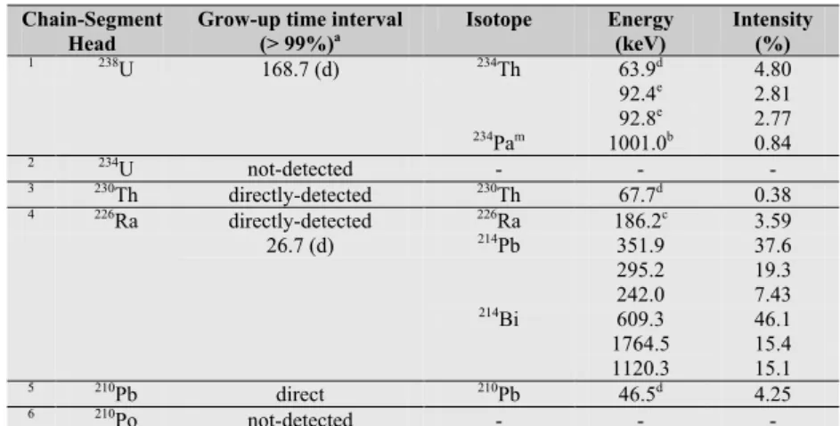
However, in the study of uranium decay chain through gamma-ray spectrometry techniques it is important to emphasize that some long lived radionuclides (238U, 226Ra, 210Pb) can be the head of decay
chain segments which can be directly measured or through secular equilibrium grow-up conditions in less than one year. The segments of 234U and 210Po can not be measured under the above mentioned
conditions.
In Table 1.2 are listed the principal isotopes which may form decay chain segments in uranium decay
chain, and used to study the secular equilibrium through gamma-ray spectrometry measurements. For each segment chain are indicated the isotopes which can be detected using gamma-ray spectrometry measurements and the grow-up time.
Table 1.2: heads of decay chain segments in uranium decay chain and the respective grow-up times.
Chain-Segment Head
Grow-up time interval
(> 99%)a Isotope Energy (keV) Intensity (%)
1 238U 168.7 (d) 234Th 63.9d 4.80 92.4e 2.81 92.8e 2.77 234Pam 1001.0b 0.84 2 234U not-detected - - - 3 230Th directly-detected 230Th 67.7d 0.38 4 226Ra directly-detected 226Ra 186.2c 3.59 26.7 (d) 214Pb 351.9 37.6 295.2 19.3 242.0 7.43 214Bi 609.3 46.1 1764.5 15.4 1120.3 15.1 5 210Pb direct 210Pb 46.5d 4.25 6 210Po not-detected - - -
a Grow-up time (>99%) calculated as 7 time half-life of the longest lived isotope of the chain-segment. b Low yield gamma energy.
c Generally recorded as a doublet with 185.7 keV (235U).
d Low energy (requires n-type HPGe detector for best sensitivity and accuracy). e Recorded as doublet between 92.4 keV and 92.8 keV from 234Th.
Thorium
Natural thorium has only one primordial isotope that of 232Th having an natural isotopic ratio of 100%. The decay chain of 232Th includes 6 alpha decays and 4 beta decays respectively (Fig. 1.4), often
natural decay chains, as follows: 234Th (24.1 d half-life) and 230Th (7.54 104 y half-life) in the 238U chain; 228Th (1.9 y half-life) in the 232Th chain; and 231Th (1.06 d half-life) in the 235U chain.
Generally thorium and it’s daughters are found in secular equilibrium. However, in 232Th decay chain
the two chain segments having on head 228Ra and 228Th reach the secular equilibrium in about one month (Table 1.3). Thorium occurs in the tetravalent (Th4+) oxidation state and is insoluble except at
low pH (near-neutral), or in the presence of organic compounds such as humic acids (Langmuir and
Herman 1980). At near-neutral pH and in alkaline soils, the precipitation of thorium as a highly
insoluble hydrated oxide phase and the co-precipitation with hydrated ferric oxides can, with sorption reactions, are two important mechanisms for the removal of thorium from solution. Because of sorption and precipitation reactions and the low solution rate of thorium-bearing minerals, thorium concentrations in natural waters are generally low. Radium (228Ra) show the same geochemical
properties as radium isotope in uranium decay chain. Thoron (220Rn) has a lesser opportunity to escape
in the atmosfere than radon isotopes (222Rn) due to its shorter half-life (55.6 s half-life). However,
particularly in the last decade, the number of researches on thoron has been increasing especially in indoor ambients. It is worth mentioning that a study carried out in China indicated that the ratio of the average equilibrium equivalent concentration of thoron progeny (EEC Tn) to that of radon progeny (EEC Rn) ranged from 0.06 to 0.13, but the range of the dose ratio (thoron progeny)/(radon progeny) was between 0.31 and 0.47 (Guo et al. 2005). This ratio indicates that the dose from thoron progeny may be not negligible for radiological purposes.
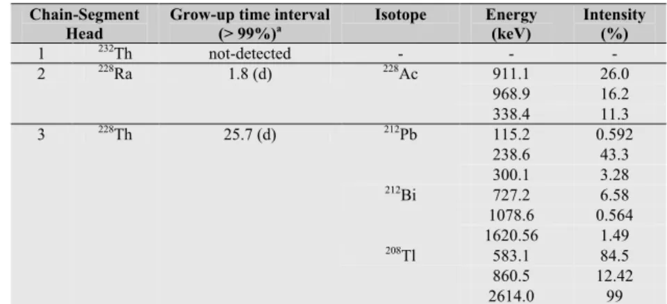
In table 1.3 are listed the principal isotopes which may form decay chain segments in thorium decay chain, and used to study the secular equilibrium through gamma-ray spectrometry measurements. For each segment chain are indicated the isotopes which can be detected using gamma-ray spectrometry measurements and the grow-up time.
Table 1.3: heads of decay chain segments in thorium decay chain and the respective grow-up times.
Chain-Segment Head
Grow-up time interval
(> 99%)a Isotope Energy (keV) Intensity (%)
1 232Th not-detected - - - 2 228Ra 1.8 (d) 228Ac 911.1 26.0 968.9 16.2 338.4 11.3 3 228Th 25.7 (d) 212Pb 115.2 0.592 238.6 43.3 300.1 3.28 212Bi 727.2 6.58 1078.6 0.564 1620.56 1.49 208Tl 583.1 84.5 860.5 12.42 2614.0 99
a Grow-up time (>99%) calculated as 7 time half-life of the longest lived isotope of the chain-segment.
Terrestrial absorbed dose rate coming from external gamma radiation
For health protection purposes the absorbed dose rate coming from the external gamma radiation can be calculated by knowing the activity concentrations in soil using a simple formula:
1
( ) K K U U Th Th
D nGy h C S C S C S (Eq. 1.1)
where STh, SU, and SK are the dose conversion coefficients for Th, U, and K, respectively (Table 1.4)
and CTh is the activity concentration measured through the 208Tl photo-peak (in Bq/kg), CU is the
activity concentration measured through the 214Bi photo-peaks (in Bq/kg), and C
K is the activity
concentration measured through the 40K photo-peak (in Bq/kg). In general the estimates of uranium
and thorium concentration is based on the assumption of equilibrium conditions through the direct measurement of daughter isotopes and therefore usually reported as “equivalent uranium” (eU) and “equivalent thorium” (eTh).
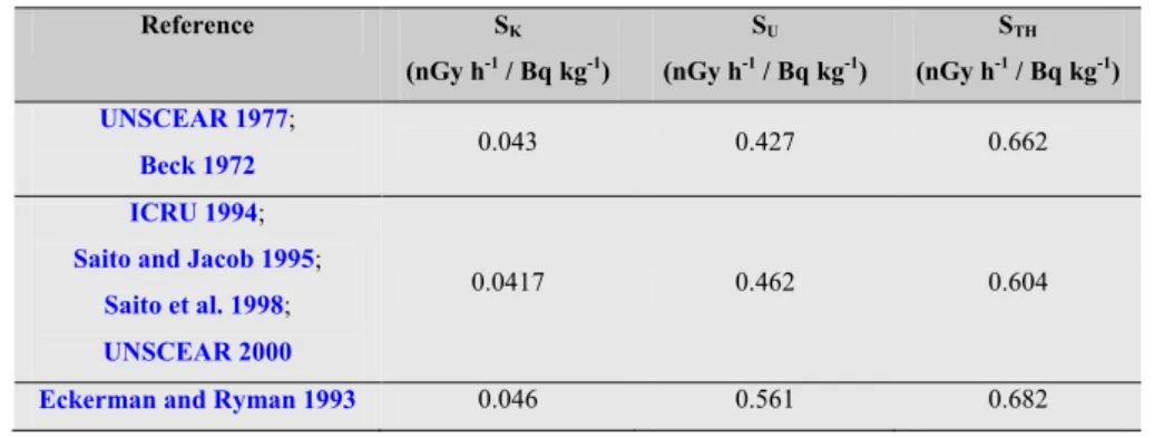
Table 1.4 shows the evolution of dose conversion coefficients in nGy/h per Bq/kg as reported by the
United Nations Scientific Committee on the Effects of Atomic Radiation (UNSCEAR 2000) and other publications. The dose coefficients listed in Table 1.4 have been used worldwide throughout the years since published. The slight differences in dose coefficients are not taken into consideration in most calculations.
Table 1.4: dose conversion coefficients for external gamma radiation coming from natural radionuclides present in soil. Reference SK (nGy h-1 / Bq kg-1) SU (nGy h-1 / Bq kg-1) STH (nGy h-1 / Bq kg-1) UNSCEAR 1977; Beck 1972 0.043 0.427 0.662 ICRU 1994;
Saito and Jacob 1995;
Saito et al. 1998;
UNSCEAR 2000
0.0417 0.462 0.604
Eckerman and Ryman 1993 0.046 0.561 0.682
1.2.2 Radioactive decay series
The natural decay series of 238U, 235U and 232Th are an example of natural radioactive decay series and
therefore are briefly discussed in this section. Radioactive decay series (or chain) often occurs in a number of daughter products, which are also radioactive, and terminates in a stable isotope
( )A ( )B ( )
A B C stable . Assuming that at time t = 0 we have
0
A
N atoms of the parent element
and no atoms of the decay product are originally present, the number of parent nuclei decrease with time according to the Eq 1.2.
A A A dN N dt (Eq. 1.2) where 0 A t A A N N e (Eq. 1.3)
While the number of daughter nuclei increases (grow-up) as a result of decays of the parent and decreases as a result of its own decay:
B
A A B B
dN
N N
The solution of the first order differential equation ( / ) 0 At
B B B A A
dN dt N N e is of the form
At Bt
B
N Ae Be and by substituting into the above equation with the initial conditions described above we find: 0 ( At Bt) A A B B A N N e e (Eq. 1.5)
From equations 1.3 and 1.5 can be calculated the relative activity ratio of the two species:
( ) 1 B A t B B B A A B A N e N
- AB: in the case when the half-life of nuclide A is much greater than the half-life of nuclide B, so the parent decays at constant rate we have:
0(1 B )
t
BNB ANA e
This equation express the secular equilibrium condition, where as t becomes large nuclei B decay at the same rate at which they are formed: BNBANA0. This result can also be immediately obtained form equation 1.4, taking dNB/dt . For practical purposes, equilibrium may be considered 0 established after seven daughter half-lives (more than 99% of daughter nuclides grow-up) (Fig. 1.5).
Figure 1.5: secular equilibrium buildup of a very short-lived daughter (222Rn of half-life 3.824 d) from a long-lived parent (226Ra of half-life 1600 y). The activity (arbitrary unit) of the parent remains constant, while the activity of the daughter reaches secular equilibrium (more than 99%) just after seven half-lives.
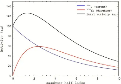
- AB: as t increases, the exponential term becomes smaller and the activity ratio (AB/A ) A
approaches the limiting constant value B/ (BA). The activities themselves are not constant, but the nuclei of type B decay (in effect) with the decay constant of type A. This situation is known as
transient equilibrium condition (Fig. 1.6).
Figure 1.6: transient equilibrium of the decay of 234U (of half-life 2.45 x 10⁵ y) to 230Th (of half-life 7.54 x 10⁴ y). The
activity ratio daughter/parent approaches the constant value 1.48.
- A B: in the case when the parent decay quickly, (A B), and the daughter activity rises to a maximum and then decays with its characteristic decay constant, if t is so long the number of nuclei type A is small (eAt 0): ( / ) Bt
BNB B ANA A B e
, which reveals that the type B nuclei decay approximately according to the exponential law (Fig. 1.7). An example of no equilibrium condition, is the nuclear fission product series containing 90Sr which is largely studied for
environmental radioprotection purposes:
Figure 1.7: no equilibrium: the growth and decay of 90Rb (of half-life 158 s) from 90Kr (of half-life 33.33 s). If 90Kr is not continuously produced it will vanish more quickly producing 90Rb which on turn will vanish quickly respective 90Sr having a much longer half-life and reaching secular equilibrium with its daughter 90Y.
Another example of no-equilibrium condition is the growth of 235U (7.04 x 10⁸ y) from 239Pu (2.41 x
104 y): indeed the head isotope of this decay chain is 235U.
1.3 Man-made radionuclides
Fallout from atmospheric weapon testing and from NPP accidents
Over 2000 nuclear tests distributed all over the world from 1945 to 1998 gave rise to the atomic age causing a global radiological contamination. The estimated global release of 137Cs and 131I from
atmospheric nuclear weapon testing were respectively 9.48 x 10¹⁷ Bq and 6.75 x 10²⁰ Bq (UNSCEAR
2008). In the figure 1.8 below are distributed the nuclear test around the world divided in atmospheric and underground regarding their yield.
Figure 1.8: the global distribution of the locations of all nuclear tests and other detonations worldwide. Atmospheric tests are in blue, underground tests in red. Successively larger symbols indicate yields from 0 to 150 kt, from 150 kt to 1 mt, and over 1 mt. Data taken from: http://www.johnstonsarchive.net/.
About 30 major NPP incidents and accidents have occurred, ranked by INES (International Nuclear and Radiological Event Scale) scale, with Chernobyl and Fukushima as the first two accidents caused more damages and contamination. There are over 440 nuclear power plants for electricity generation with 60 more NPP under construction (IAEA 2011), which operate in about 30 countries (Fig. 1.9) producing about 14% of world electricity demand.
According to INES scale (IAEA 2008) Chernobyl (1986) and Fukushima (2011) are classified as the most severe accidents occurred in nuclear power industry. Chernobyl accident caused the largest uncontrolled radioactive release into the environment; when large quantities of radioactive substances were released into the air for about 10 days. The radioactive cloud dispersed over the entire northern hemisphere, and deposited substantial amounts of radioactive material over large areas. A enormous number of studies have been undertaken in order to estimate the fallout distribution in particular the two radioanuclides, the short-lived 131I (8 d half-life) and the long lived 134Cs (2 y half-life) and 137Cs
(30 y half life) which are particularly significant for the radiation dose they deliver. In the figure below is shown the combined work of many countries showing the distribution of 137Cs all over the world
guided by European Commission Joint Research Centre (Fig. 1.10).
Figure 1.10: European map 1 : 11 250 000 of 137Cs deposition following Chernoby NPP accident. Data taken from:
http://rem.jrc.ec.europa.eu/.
Recently, Japan was hit by a 9.0 magnitude earthquake followed by a tsunami that affected hundreds of thousands of people and seriously damaged the Fukushima Daichi power plant in Japan, where radioactive emissions from Fukushima spread across the entire northern hemisphere. Fukushima nuclear power plant accident was classified as INES scale 6 regarding to Chernobyl (INES scale 7). In
2008) which can be compared with Fukushima first data received, showing about one order of magnitude differences between them.
Table 1.5: principal radionuclides released (volatile elements) in Chernobyl accident compared to those assumed from
Fukushima Dai-ichi accident.
Radionuclide Half-life
Activity released (1015 Bq)
Chernobyl UNSCEAR 2008
Fukushima Dai-ichi (NISA) http://www.nisa.meti.go.jp/ Fukushima Dai-ichi (NSC) http://www.nsc.go.jp/ 131I 8.04 d ~1760 130 150 134Cs 2.06 y 47 - - 137Cs 30.0 y ~85 6.1 12
Chapter
2
Laboratory γ-ray spectrometry: a fully
automated low-background high-resolution
γ-ray spectrometer
MCA_Rad system composed by two coupled HPGe detectors accurately shielded and an automatic sample changer driven by electromechanical pistons using compressed air.
2.1 MCA_Rad system: set-up design and automation
2.1.1 Features of HPGe detectors 2.1.2 Shielding design and evaluation 2.1.3 Automation: hardware and software developments
2.2 MCA_Rad system calibration
2.2.1 Energy calibration
2.2.2 Efficiency calibration with uncertainty budged
2.3 Case of study: bedrock radioelement mapping of Tuscany Region
2.3.1 Representative sampling strategy and sample preparation 2.3.2 Summary of the results: mapping of radioelements
2.4 Appendix A: calculation of simplified coincidence summing correction factor for 152Eu