Deep Learning for computer-aided detection and diagnosis of clustered microcalcifications on digital mammograms

(1)

UNIVERSITÀ DEGLI STUDI DI

CASSINO E DEL LAZIO MERIDIONALE

Corso di Dottorato in

Metodi modelli e tecnologie per l’Ingegneria

curriculum Ingegneria dell’informazione

Ciclo XXXII

Deep Learning for computer-aided detection and diagnosis of

clustered microcalcifications on digital mammograms

SSD:ING-INF/05

Coordinatore del Corso

Chiar.ma Prof.ssa Wilma Polini Dottoranda Benedetta Savelli Supervisore

(2)

accompagnato in questo meraviglioso percorso di

vita...

(3)

Abstract

Breast cancer is one of the most common cause of cancer death in women worldwide. In most western countries, screening programs are organized in order to detect breast cancers at an early stage. To improve breast cancer detection, many radiologists use computer-aided detection and diagnosis (CAD) systems which are able to detect and characterize mammographic signs of malignancy such as clustered microcalcifications and masses through computerized image analysis. Even though effective in terms of sensitivity, these systems produce a too high number of false alarms, which potentially limits the benefit they can provide. This thesis addresses the problem of accurately detecting and classifying clustered microcalcifications in full field digital mammograms. The goal is to reduce the gap between CAD systems and radiologists in terms of false alarms while maintaining the high sensi-tivity typical of the commercial CAD systems. To this end, three main con-tributions are proposed by exploiting innovations and advantages of novel machine learning algorithms, based on deep learning convolutional neural networks (CNNs) : (i) a new proposal of combination of a deep cascade of boosting classifiers and a CNN to deal with the high-imbalance problem of classifying individual pixels in a mammogram as belonging to a microcal-cification or not; (ii) a novel method for detecting individual calmicrocal-cifications that provides for the use of multiple-depth CNNs, to exploit both the local features and the surrounding context of MCs; and (iii) a novel end-to-end system able to combine both detection and classification of malignant clus-ter, by additionally segmenting individual calcifications. Along with these contributions, experimental comparisons with other existing methods in the literature are provided and show significant reduction in the number of false alarms. Moreover a novel end-to-end model that combines detection and classification steps is presented, by showing a significant improvement with

respect to single-task systems. When applied to a clinical setting, this

would help the radiologists to reduce the number of unnecessarily recalled women with microcalcification clusters, thus improving the effectiveness of screening and diagnosis processes.

(4)

(5)

List of Figures

1.1 (a) Anatomy of the breast: (1) chest wall, (2) pectoralis

muscles, (3) lobules, (4) nipple, (5) areola, (6) milk ducts, (7) fat and connecting tissue, (8) skin. (b) Terminal duc-tal lobular unit. (c) Lobular calcifications. (d)

Intraduc-tal calcifications. Source: www.wikipedia.org and www.

radiologyassistant.nl. . . 3

1.2 (a) Lobular Carcinoma In Situ (LCIS): (1) normal lobular cells, (2) lobular cancer cells. (b) Different stages of can-cer cells growing from the milk ducts: (I) normal cells, (II) Ductal Carcinoma In Situ (DCIS), (III) Invasive Ductal Car-cinoma (IDC). Source: www.breastcancer.org. . . 4

1.3 (a) Mammography apparatus : (1) anode, (2) filter, (3) X-rays, (4) compression plate, (5) scattering, (6) grid, (7) re-ceptor. . . 8

1.4 (a)(b) Standard digital mammography exam with cranio-caudal (right) and mediolateral oblique (left) views of both breasts (source: The Breast Journal). . . 9

1.5 (a) Characteristic curve of a mammographic screen-film sys-tem. (b) Characteristic response of a detector designed for digital mammography. . . 9

1.6 Classification of breast calcifications into benign, suspicious and malignant types basing on their distribution . . . 12

1.7 Classification of breast calcifications into benign, suspicious and malignant types basing on their distribution . . . 13

1.8 An example of an ROC curve . . . 16

2.1 An example of deep feed forward neural network . . . 20

2.2 ReLu activation function . . . 22

2.3 Stochastic Gradient descent: the role of learning rate . . . . 23

2.4 Stochastic Gradient descent: the role of momentum . . . 24

2.5 Comparison between a standard deep neural network and the same network with dropout application. The circles with a cross symbol inside denote deactivated units. . . 25

2.6 Convolutional neural network with two convolutional layers, one pooling layer and one dense layer. The activations of the last layer are the output of the network. . . 26

2.7 Illustration of translation invariance in convolutional neural network. The bottom leftmost input is a translated version of the upper leftmost input image by pixel right and one-pixel down. . . 27

(10)

2.8 VGGnet configurations. The depth of the congurations in-creases from the left (A) to the right (E), as more layers are

added. Source: Simonyan et al. [48] . . . 29

2.9 U-net architecture (example for 32x32 pixels in the lowest

resolution). Each blue box corresponds to a multi-channel feature map. The number of channels is denoted on top of the box. The x-y-size is provided at the lower left edge of the box. White boxes represent copied feature maps. The arrows denote the different operations. Source: Ronneberger

et al. [56] . . . 30

3.1 The Haar-like feature groups used by the cascade of

classi-fiers. (a) Some examples of the first group. (b) An example

of the second group. (c) Some examples of the third group. . 34

3.2 Overview of the proposed MC detection scheme. On the

left, Deep Cascade reduces the class imbalance ratio in the

input data by about three orders of magnitude. This is

achieved thanks to a sequence of five high-sensitivity classi-fiers that linearly combine a large number of decision stumps constrained to use single Haar-like features (top row in each classifier’s box). The remaining samples are then classified by a VGGNet inspired CNN and assigned a probability score

using the output from the last fully connected layer. . . 36

3.3 Average ROC curves obtained from 1, 000 bootstrap

itera-tions. Confidence bands indicate 95% confidence intervals

along the TPR axis. . . 40

4.1 Overview of the proposed architecture . . . 43

4.2 Details of the proposed architecture . . . 45

4.3 Chart describing the findings in the INbreast database . . . 46

4.4 Some examples of images from (a-b) INbreast . . . 47

4.5 InBreast annotation example . . . 48

4.6 Average ROC curves obtained from 1, 000 bootstrap

iter-ations for INbreast dataset.Confidence bands indicate 95%

confidence intervals along the TPR axis. . . 50

4.7 FROC curves for (a) INbreast dataset . . . 51

5.1 Hard parameter sharing for multi-task learning in deep neural

networks . . . 57

5.2 Soft parameter sharing for multi-task learning in deep neural

networks . . . 58

5.3 Overview of the proposed method . . . 60

5.4 DIAG dataset annotation example . . . 63

5.5 Comparison image-based FROC curves of a basic U-Net for

detection and of the proposed modified U-Net for detection

and classification . . . 66

5.6 Comparison case-based FROC curves of a basic U-Net for

detection and of the proposed modified U-Net for detection

and classification . . . 67

5.7 Comparison image-based ROC curves of a U-Net for

classifi-cation and of the proposed modified U-Net for detection and

(11)

LIST OF FIGURES

5.8 Image-based FROC curves obtained for single and joint

pre-dictions . . . 68

5.9 Example of a True Positive detected cluster . . . 72

(12)

(13)

List of Tables

2.1 A list of commonly applied last layer activation functions for

various tasks . . . 26

3.1 Architecture of the VGGNet-based CNN . . . 38

3.2 Comparative results of mean MC detection sensitivity S . . 39

3.3 Average per-mammogram processing time . . . 39

4.1 Details of the incremental block . . . 44

4.2 Details of the classification block . . . 44

4.3 Results of mean MC detection sensitivity S for standalone

CNNs . . . 49

4.4 Results of mean MC sensitivity S for combined CNNs . . . . 49

4.5 Results of MC sensitivity S for combined CNNs according to

different combination rules . . . 49

4.6 Comparative results of mean MC detection sensitivity S . . 51

4.7 Comparative results of the FROC score and sensitivities at

specific FPpI . . . 52

4.8 Results of MC per-image processing time for the trained

net-works . . . 52

5.1 Details of the classification block . . . 59

5.2 Distribution of the digital mammography (DM) exams

in-cluded in this study. . . 62

(14)

(15)

Chapter 1 Introduction

Worldwide, breast cancer is the most common cancer (24.2%) and the first known cause of death (13,7%) among women aged between 35 and 55 [1]. Detecting breast cancer as early as possible is vital to improve patient’s chances and quality of life after treatment. With this aim, population-based screening program started in the late 70s and have been adopted as organized nation-wide programs in many developed countries since then. In the screening programs asymptomatic women within a certain age range are regularly invited (every year or every two years) to obtain a screening exam. It is important to underline that the positive effects of screening are mainly due to the principle of repetition. For this reason, the first round should be considered differently from the repeated rounds and monitored and reported separately.

The chosen technique for screening mammography, is a noninvasive and relatively cheap test which uses x-rays to obtain a two-dimensional(2D) image of the breast. Although using ionizing radiation, the risk for an average 50 year old woman to develop cancer from a mammography exam is estimated to be about 9 in 10000 [2]. Screen film mammography was initially used, until it was replaced by digital mammography (DM) in the mid-2000s, showing an improvement in breast cancer detection accuracy, especially for women with dense breasts [3].

The large number of acquired screening mammograms are interpreted by radiologists, who look for mammographic indicators of cancer like clusters of microcalcifications (MCs) and masses, and subsequently make a final deci-sion whether the woman has to be recalled for further assessment. However, interpreting screening mammograms is a big challenge even for an expert radiologist since the low prevalence makes finding abnormalities difficult. In [4] are pointed out several subjective factors that may lead to a lack of perception or to mistakes in interpretation. Among the established methods to improve radiologist performance, it has been reported that having more than one radiologist or a CAD system improves the detection of cancer in mammograms [5, 6]. It is common practice that each woman’ screening exam is reviewed by two readers, in an independent double reading fashion. If the two radiologists disagree, the final decision on the need to recall the woman can be either by consensus of the two radiologists, by arbitration by a third radiologist, or the woman can be recalled if either of the two radiolo-gists decides that a recall is warranted. If recalled, the woman is referred to go to a hospital for further tests (diagnostic work-up). Double reading and therefore combining assessments by two or more readers improves overall

(16)

performance. However several studies have shown that unfortunately up to 25% of mammography detectable cancers are still missed at screening even after double reading [7, 8].Consequently in the last few decades, Computer-Aided Detection and Diagnosis (CADe/CADx) systems have been proposed to assist radiologists in finding and locating abnormalities on the images and supporting their diagnosis response [9, 10].To this end, several commercial CAD systems are nowadays available and their use is widespread among radiologists. However, even though CAD systems show a sensitivity similar to radiologists [11], there are still a few hundred false positives for every true positive in a screening setting, which is about two orders of magni-tude higher than what the radiologists achieve [5]. This can potentially limit the benefit that a CAD system can provide, for example by resulting in an increase of the recall rate [5] and subsequently of the false positive case (i.e., patients that are recalled unnecessary), thus causing unnecessary anxiety and thereby discouraging women to participate to screening and generating lack of trust of the readers towards CAD [12]. Nevertheless, the recent developments in Artificial Intelligence techniques for Computer Vi-sion tasks, in particular Deep Neural Networks, have brought their positive effects also in the medical image field, showing to be very effective for med-ical image analysis tasks [13, 14, 15]. As a consequence a new generation of CADe/CADx has been enabled with new solutions and perspective for digital mammograms tools [16, 17].

The objective of the studies described in this thesis is to develop a full CAD system for the detection and diagnosis of clusters of MCs, able to reduce the gap between CAD systems and radiologists in terms of false positives while maintaining the high sensitivity typical of commercial CAD

systems. In this way, the effectiveness of CAD in assisting radiologists

in screening could be improved to avoid unnecessary and invasive further work-ups in healthy women as it still happens nowadays. In this chapter an overview of the framework in which this research has been carried out is provided. Starting from a short description of the breast anatomy and the breast diseases, particular emphasis is given to the presence of suspicious and malignant MCs as one of the most important early indicator of breast cancer in mammography. Subsequently, a more detailed description of CAD system and evaluation metrics is given. Finally, an outline of the thesis is presented.

1.1 Anatomy of the breast

Anatomically the breast can be subdivided into the following structural entities [18, 19, 20]:

Chest wall

The boundary of the thoracic cavity (see Fig. 1.1a-1). Pectoralis muscles

Thick, fan-shaped muscles, situated at the chest (anterior) of the hu-man body (see Fig. 1.1a-2).

Lobules

The basic functional unit in the breast is the lobule, also called the tdlu (see Fig. 1.1a-3). The tdlu consists of 10-100 acini, that drain

(17)

1.1 Anatomy of the breast

(c)

(d)

(b)

(a)

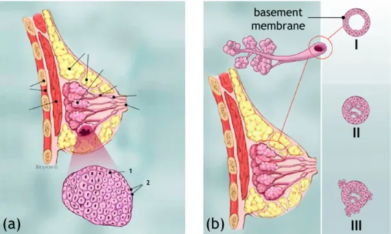
with calcifications

Figure 1.1: (a) Anatomy of the breast: (1) chest wall, (2) pectoralis mus-cles, (3) lobules, (4) nipple, (5) areola, (6) milk ducts, (7) fat and

con-necting tissue, (8) skin. (b) Terminal ductal lobular unit. (c) Lobular

calcifications. (d) Intraductal calcifications. Source: www.wikipedia.org and www.radiologyassistant.nl.

into the terminal duct (see Fig. 1.1b). The terminal duct drains into larger ducts and finally into the main duct of the lobe (or segment), that drains into the nipple. The breast contains 15-18 lobes, each containing 20-40 lobules. The tdlu is an important structure because most invasive cancers arise from the tdlu. It is also the site of origin of dcis, lcis, fibroadenoma and fibrocystic disease, like cysts, apocrine metaplasia, adenosis and epitheliosis. Most calcifications in the breast form either within the acini (lobular calcifications, see Fig. 1.1c) or within the terminal ducts (intraductal calcifications, see Fig. 1.1d). Nipple

A small projection of skin containing the outlets for 15-20 lactiferous ducts arranged cylindrically around the tip (see Fig. 1.1a-4). The skin of the nipple is rich in a supply of special nerves that are sensitive to certain stimuli. The physiological purpose of nipples is to deliver milk to the infant, produced in the female mammary glands during lactation.

Areola

Pigmented area around the nipple (see Fig. 1.1a-5). Milk duct

Milk ducts (or lactiferous ducts) form a tree branched system con-necting the lobules of the mammary gland to the tip of the nipple (see Fig. 1.1a-6). They are the structures which carry milk toward the nipple in a lactating female.

(18)

(a)

(b)

1 2

I

II

III

basement membrane

Figure 1.2: (a) Lobular Carcinoma In Situ (LCIS): (1) normal lobular cells, (2) lobular cancer cells. (b) Different stages of cancer cells growing from the milk ducts: (I) normal cells, (II) Ductal Carcinoma In Situ (DCIS), (III) Invasive Ductal Carcinoma (IDC). Source: www.breastcancer.org.

Fat, ligaments and connective tissue

Spaces around the lobules and ducts are filled with fat, ligaments and connective tissue (see Fig. 1.1a-7). The amount of fat in the breast largely determines their size. The actual milk-producing structures are nearly the same in all women. Female breast tissue is also sensi-tive to cyclic changes in hormone levels. Younger women might have denser and less fatty breast tissue than do older women who have gone through menopause.

1.2 Malignant breast diseases

Malignancy can grow within all types of breast tissue, but in the classical sense breast cancer originates in either the milk-ducts, in which breast milk is transported to the nipple, or the lobules, where breast milk is produced. Several types of breast cancer can arise in other parts of the breast as well, but are less common (< %8 of all breast cancers). The basement membrane (see Fig. 1.2) plays a key role in determining whether a carcinoma is “in situ” (i.e., it has not grown through the basement membrane) or “invasive” (i.e., it has grown through the basement membrane). When in situ carcinomas develop into invasive cancers, they can form metastases to lymph nodes and other organs which will decrease the survival chance. In the breast the following forms of malignancy can be considered [21]:

Lobular Carcinoma In Situ (LCIS)

LCIS is an area (or areas) of abnormal cell growth in the lobule (see Fig. 1.2a). The abnormal cells start growing in the lobules and remain inside the lobule without spreading to surrounding tissues. People

(19)

1.2 Malignant breast diseases

diagnosed with LCIS tend to have more than one lobule affected. Despite the fact that its name includes the term “carcinoma”, LCIS is not a true breast cancer. Rather, LCIS is an indication that a person is at higher-than-average risk for getting breast cancer at some point in the future.

LCIS is usually diagnosed before menopause, most often between the ages of 40 and 50. Less than 10% of women diagnosed with LCIS have already gone through menopause. LCIS does not cause symptoms and usually does not show up on a mammogram. It tends to be diagnosed as a result of a biopsy performed on the breast for some other reason. Invasive lobular Carcinoma(ILC)

ILC is the second most common type of breast cancer after Invasive Ductal Carcinoma (IDC). The cancer begins in the milk-producing lobules and breaks through the wall of the lobule thus invading the tissues of the breast. Over time, ILC can spread to the lymph nodes and possibly to other areas of the body. About 10% of all invasive breast cancers are invasive lobular carcinomas. ILC tends to occur later in life than Invasive Ductal Carcinoma (IDC): the early 60s as opposed to the mid to late 50s. At first, ILC may not cause any symptoms. Sometimes, an abnormal area turns up on a screening mammogram, which leads to further testing. ILC tend to be more difficult to see on mammograms than IDC are. That is because in-stead of forming a lump, the cancer cells more typically spread to the surrounding connective tissue in a line formation.

Ductal Carcinoma In Situ (DCIS)

DCIS is the most common type of non-invasive breast cancer and it represents the 25-30% of all reported breast cancers [20]. The cancer starts inside the milk ducts and remain in the ducts without spread-ing to the surroundspread-ing tissues (see Fig. 1.2b-II). DCIS is not life-threatening, but having DCIS can increase the risk of developing an invasive breast cancer later on. When a woman has had DCIS, she is at higher risk for the cancer coming back or for developing a new breast cancer than a woman who has never had breast cancer before. Most recurrences happen within the 5 to 10 years after diagnosis. The chances of a recurrence are under 30%. DCIS generally has no signs or symptoms. A small number of women may have a lump in the breast or some discharge coming out of the nipple. However, approximately 95% of all DCIS is diagnosed because of mammographically detected microcalcifications [20], making it the most easily detectable cancer in mammography among the early stages of cancer.

Invasive Ductal Carcinoma(IDC)

IDC is the most common type of breast cancer. About 80% of all breast cancers are IDC. The cancer starts inside the milk ducts and breaks through the wall of the duct thus invading the tissues of the breast (see Fig. 1.2b-III). Over time, IDC can spread to the lymph nodes and possibly to other areas of the body. Although IDC can affect women at any age, it is more common as women grow older. According to the American Cancer Society, about two-thirds of women are 55 or older when they are diagnosed with an IDC. At first, IDC

(20)

may not cause any symptoms. Often, an abnormal area (mass) turns up on a screening mammogram, which leads to further testing.

1.3 Breast imaging

Imaging of the breast is currently done using either X-ray (mammography, tomosynthesis,CT), sound waves or radio waves:

• Mammography: Mammography involves exposing the breast to a

small dose of ionizing radiation. The breast is placed in a C ark

between an X-ray source emitting radiation and a detector.

• Tomosynthesis: Similar to mammography, tomosynthesis is based on X-ray. In this case the x-ray tube moves in an arc over the compressed breast, by capturing multiple images of each breast from different angles. The digital images are then reconstructed or “synthesized” into a set of three-dimensional images to get a better view of structures that would otherwise be hidden. The dose of radiation is slightly higher tough within the limits of safe radiation outlined by the FDA. • Breast CT: Similar to mammography and tomosynthesis, breast CT is based on X-ray, but instead images are taken from many different an-gles so as to create a full 3D reconstruction of the breast, where voxels have a quantitative meaning. Breast CT still has limited application in the clinic.

• Breast Ultrasound : Ultrasound devices use soundvawes to produce an image of the internal structure of the breast. Ultrasound is typi-cally used as a complementary modality to mammography to diagnose lumps that were found suspicious on mammogram. Ultrasound can not look as deep inside the breast as mammography can, does not image the whole breast at once and can not see all indications (such as calcifications) that are visible on a mammogram. Is therefore un-suitable for stand-alone imaging.

• Magnetic Resonance Imaging: MRI uses magnetic fields and radiowaves to generate images of internal structure. Similar to breast ultrasound, calcifications in the breast are typically not visible in MRI. It is often used as complementary to a mammogram for women in high risk pop-ulations. The sensitivity of readers is substantially higher, but MRI is also substantially more expensive than mammography and in general with lower specificity.

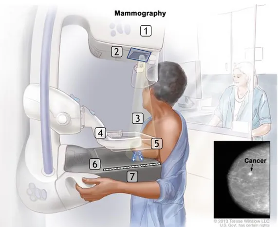
1.3.1 Mammography

Mammography is the oldest and still most common breast imaging tech-nique that is used to detect and characterize breast cancer thanks to its high performance and low costs [22, 5, 23] and are used both for screening and diagnostic purposes. In general, screening mammography is performed on asymptomatic women to identify suspicious signs at an early, and there-fore more treatable stage. Diagnostic mammography is performed on symp-tomatic patients, or to work up abnormalities found on screening images.

(21)

1.3 Breast imaging

Hence, the aim is to characterize the pathology and define a diagnosis. In a standard examination, two images of each breast are taken: one from the top, called craniocaudal (CC) and one with the X-ray tube angled

approxi-mately 45◦ medially, called mediolateral oblique (MLO). This ensures that

the images display as much breast tissue as possible. An overview of the mammography apparatus is given in Fig. 1.3. X-ray photons are emitted from the anode that is located in the X-ray tube on the top of the machine. Whereas most x-ray tubes use tungsten as the anode material, mammogra-phy equipment uses molybdenum anodes or in some designs, a dual material anode with an additional rhodium track. These materials are used because they produce a characteristic radiation spectrum that is close to optimum for breast imaging. After x-ray photons are emitted, they pass through a molybdenum (or rhodium) filter to reduce unnecessary exposure to the patient and also to improve contrast sensitivity. Part of the radiation then goes through the breast, which is compressed primarily to spread the breast tissue laterally in order to minimize the likelihood of occult cancers, and secondarily to reduce the thickness of the breast thus obtaining a clear x-ray image. As a result of interaction between breast tissue and radiation, X-ray photons may undergo a change in direction before hitting the receptor. By positioning a grid in front of the receptor, influence of scatter is reduced. Both film/screen and digital receptors are used for mammography, thus obtaining Screen-Film Mammography (SFM) and Full-Field Digital Mam-mography (FFDM) (see Fig. 1.3c), respectively, whose characteristics are detailed in the following.

1.3.2 Screen-film mammography

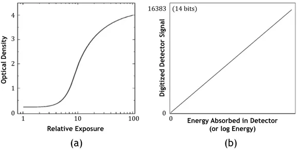
In screen-film based mammography, the radiation is absorbed by a scintilla-tor (the screen) that transfers the incident X-ray photons into light photons that blacken the film, which is located just in front of the screen. The film serves as the media for recording within the receptor, transporting and stor-ing images, and is the image display device. The significant characteristic is that the contrast of the image is “fixed” and cannot be changed after the film is exposed and chemically processed. In addition, the relation between optical film density and exposure values is non-linear (see Fig. 1.5a) and depends on the type of film used. For these reasons, it has been shown that although SFM has high sensitivity and specificity, it has some important limitations as well [24, Chapter 1]. The film used to capture, store and dis-play the mammographic image is one of the major technical restrictions of SFM. The visibility of breast cancer depends on different attenuation of the X-ray beam by the suspect regions compared with the surrounding tissue. Suspect regions lying in dense areas of the breast may not be noticeable because film contrast decreases in the densest breast areas. This is due to limited dynamic range of conventional films. Furthermore, the image data obtained using a SFM-based system cannot be manipulated once the im-age is processed in a film processor. Specifically, over- and under-exposed images have to be recorded again. Contrast levels in the image cannot be altered to improve the relative visibility of structures in the image without recording additional images of the patient. Most of the several technical lim-itations associated with SFM are overcame by FFDM, which is described in the following section.

(22)

Figure 1.3: (a) Mammography apparatus : (1) anode, (2) filter, (3) X-rays, (4) compression plate, (5) scattering, (6) grid, (7) receptor.

1.3.3 Full-field digital mammography

In the last few years, FFDM-based systems have been developed and are increasingly used in clinical practice. In FFDM, the radiation is captured by a digital detector that inherently produces a signal that is linearly pro-portional to the intensity of X-rays transmitted by the breast (see Fig. 1.5). There are several key features of FFDM that distinguish it from SFM and contribute to its potential advantages [24, Chapter 1]. First of all FFDM decouples the processes of image acquisition from the subsequent stages of archiving, retrieval, image display and digital image processing. Unlike the situation in SFM where these processes are inextricably linked, this facili-tates optimization of each of the separate functions and great flexibility in the adjustment of image display characteristics. Secondly FFDM it is often possible to design detectors that allow efficient use of the incident X-rays without excessive loss of spatial resolution and signal to-noise ratio. This permits a substantial reduction in the radiation dose to the breast when compared with SFM without sacrifice of image quality. Moreover, because of the differences in technology between SFM and FFDM, the optimum ex-posure conditions may shift toward the use of higher energy spectra than would be used with film, particularly for dense or thick breasts. In an SFM-based system, the relation between optical film density and exposure values is highly non linear and it tends to flatten for exposures above and below a fairly restricted range (see Fig. 1.5a). This limited range has important implications on image quality [24, Chapter 1]. On the contrary, in FFDM

(23)

1.4 Signs of breast cancer in mammography

Figure 1.4: (a)(b) Standard digital mammography exam with craniocaudal (right) and mediolateral oblique (left) views of both breasts (source: The Breast Journal).

(a)

(b)

0 16383 (14 bits) 0 1 2 3 4

1 10 100 Energy Absorbed in Detector (or log Energy)

Relative Exposure Di gi ti ze d De te cto r Si gn al Opti ca l De ns ity 0

Figure 1.5: (a) Characteristic curve of a mammographic screen-film system. (b) Characteristic response of a detector designed for digital mammography.

the detector inherently produces a signal that is linearly proportional to the intensity of X-rays transmitted by the breast (see Fig. 1.5b). It has a very large dynamic range, so that it is possible to produce a faithful representa-tion of X-ray transmission for all parts of the breast.

1.4 Signs of breast cancer in mammography

The main signs of malignancy on mammography can roughly be divided into two groups: microcalcifications and soft tissue lesions[25].

1.4.1 Microcalcifications

Microcalcifications are calcium deposits that appear as small white specks on the mammogram. Typical size of a MCs is between 0.1 mm and 1 mm

(24)

[26] and they may appear scattered over the whole breast or distributed in one or more clusters. Microcalcification clusters may appear in both in situ and invasive breast cancer but also in benign diseases. Many of the breast cancers that are at an early stage are currently detected by the presence of microcalcifications. Approximately 95% of all DCIS is diagnosed because of mammographically detected microcalcifications [20].

Most calcifications in the breast form either within the TLDU (intra-ductal calcifications) or within the acini (lobular calcifications) [20]. More details on these two types of calcifications are given in the following. Lobular calcifications

These calcifications fill the acini, which are often dilated (see Fig. 1.1c). This results in uniform, homogeneous and sharply outlined calcifica-tions, that are often punctate or round. When the acini become very large, as in cystic hyperplasia, “milk of calcium” may fill these cav-ities. However when there is more fibrosis, as in sclerosing adenosis, the calcifications are usually smaller and less uniform. In these cases it can be difficult to differentiate them from intraductal calcifications. Lobular calcifications usually have a diffuse or scattered distribution, since most of the breast is involved in the process that forms the calcifications. Lobular calcifications are almost always benign.

Intraductal calcifications

These calcifications are calcified cellular debris or secretions within the intraductal lumen (see Fig. 1.1d). The uneven calcification of the cellular debris explains the fragmentation and irregular contours of the calcifications. These calcifications are extremely variable in size, density and form (i.e., pleomorphic from the Greek pleion “more” and morphe “form”). Sometimes they form a complete cast of the ductal lumen. This explains why they often have a fine linear or branch-ing form and distribution. Intraductal calcifications are suspicious of malignancy.

The diagnostic approach to breast calcifications is to analyze the mor-phology, distribution and sometimes change over time.

Morphology

The form or morphology of calcifications is the most important factor in deciding whether calcifications are typically benign or not. If not, they are either suspicious (intermediate concern) or of a high probability of malig-nancy. Usually biopsy in these cases is needed to determine the etiology of these calcifications. Using morphology as classification criterion, we can distinguish microcalcifications as follows:

• Skin calcifications: these are usually lucent-centered deposits. Skin calcifications may simulate parenchymal breast calcifications and may look like malignant-type calcifications, but when looking at MLO and CC views these calcifications look exactly the same.

• Vascular calcifications: These are linear or form parallel tracks, that are usually clearly associated with blood vessels. They may simulate intraductal calcifications.

(25)

• Popcorn-like calcifications: These calcifications are produced by invo-luting fibroadenomas. They usually do not cause a diagnostic prob-lem.

• Rod-like calcifications: These benign calcifications form continuous rods that may occasionally be branching. They are different from malignant-type fine branching calcifications, because they are usually > 1mm in diameter. They may have lucent centers if the calcium is in the wall of the duct. These calcifications follow a ductal distribution, radiating toward the nipple and are usually bilateral.

• Round and punctuate calcifications: Round calcifications are 0.5 − 1mm in size and frequently form in the acini of the terminal duct lobular unit. When smaller than 0.5mm, the term punctuate is used. • Milk of Calcium: These are benign sedimented calcifications. On CC views they appear as fuzzy, round or amorphous whereas on MLO view they may appear as semilunar crescent shaped.

• Coarse irregular lava-shaped: These calcifications are larger than 0.5mm and often have a lucent center. They are seen in irradiated breast or following trauma. They develop 3 − 5 years after treatment in about 30% of women. These calcifications are also described as fat necrosis. • Amorphous calcifications: Amorphous or indistinct calcifications are defined as without a clearly defined shape or form. These calcifica-tions are usually so small or hazy in appearance, that a more specific morphologic classification cannot be determined.

• Coarse heterogeneous: Coarse heterogeneous microcalcifications, for-merly called coarse granular, are irregular, conspicuous calcifications that are generally larger than 0.5mm . They are considered to be of intermediate concern, along with amorphous microcalcifications. • Fine pleomorphic microcalcifications: These calcifications vary in size

and shapes. They are more conspicuous than the amorphic calcifica-tions. There is a 25 − 40% risk of malignancy.

• Fine linear branching: These are thin, linear or curvilinear irregular calcifications. They may be discontinuous and their appearance sug-gests filling of the lumen of a duct. They have a high probability of malignancy

Distribution

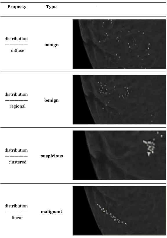
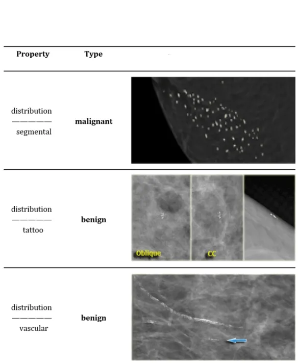
Based on the distribution calcifications can be classified as see Figs.( 1.6 1.7):

• Diffuse or Scattered: diffuse calcifications may be scattered calcifica-tions or multiple appearing throughout the whole breast. It is typi-cally seen in benign entities.

• Regional: scattered in a larger volume (> 2cc ) and not in the expected ductal distribution. Such a distribution is considered a non ductal distribution, which means associated with a benign entity.

(26)

Figure 1.6: Classification of breast calcifications into benign, suspicious and malignant types basing on their distribution

(27)

Figure 1.7: Classification of breast calcifications into benign, suspicious and malignant types basing on their distribution

(28)

• Clustered: at least 5 calcifications occupying a small volume of breast tissue. Clustered microcalcifications are seen either in benign or ma-lignant disease and are of intermediate concern. When several clusters are scattered throughout the breast tissue, this is usually considered a sign of a benign entity. On the contrary a single isolated cluster favors a malignant entity.

• Linear: calcifications arrayed in a line, suggesting deposits in a whole duct. This kind of distribution appears when DCIS fills the entire duct and its branches with calcifications.

• Segmental: calcium deposits in ducts and branches of a segment or lobe. It usually favors a ductal distribution, i.e. malignancy.

Change over time

There are conflicting data concerning the value of absence of changeover time. It is said that the absence of interval change in microcalcifications that are probably benign on the basis of morphologic criteria is a reassuring sign and an indication for continued mammographic follow-up. On the other hand in a retrospective study that included indeterminate and suspicious clusters of microcalcifications, stability can not be relied on as a reassuring sign of benignancy.

1.4.2 Soft tissue lesions

When DCIS develops into an invasive cancer, the breast cancer also becomes a soft-tissue lesion, which is the term for masses, architectural distortions and asymmetrical densities within the breast. Most soft tissue lesions have the main appearance of masses and consist of cancer cells that are more densely packed together and invades the surrounding tissue, which consists mainly of fat cells and fibrous tissue. The boundary of this type of lesion can vary between circumscribed, indistinct or spiculated. The latter type, are stellated patterns of lines that are directed towards the center of the mass. These spiculations are an important sign for malignancy of the lesion. Ar-chitectural distortions are a disruption of the normal pattern in the breast without a visible mass and are less often an invasive cancer. The asym-metrical densities, a mismatch between the density pattern between the left and right breast or acquisitions at different view angels of the breast, are also less often a malignancy.

1.5 Computer aided detection and diagnosis

The advancement of medical imaging over the past decades resulted in a big amount of medical images, with a substantial increasing of the work-load of radiologists. This is particularly true for screening programs, such as breast cancer screening , where millions of medical images are acquired each year [27, 28]. Besides the increasing workload, manual interpretation of medical images is subjective to the individual skills of radiologist and also depends on experience and their compliance with reporting guidelines.

(29)

1.5 Computer aided detection and diagnosis

For consistent reporting, different reporting systems are available for dis-eases and modalities such as the BI-RADS for breast imaging [29]. The difference in reading quality between radiologists can result in a difference in the diagnosis of a patient and can have a big impact on the number of detected cancers. For instance, a sensitivity difference varying between 18% and 40% has been observed when mammograms are read by individual breast cancer screening radiologists [30, 31]. Therefore, in many european countries, double reading has been introduced to reduce the variability in breast cancer screening performance and to increase sensitivity. However, double reading demands additional radiologists which increases their work-load even more and increases costs. Moreover the low prevalence of exams with cancer (approximately 10 per thousand women screened) within the total amount of screening examinations in fact decreases radiologists’ sen-sitivity, and therefore even double reading might not be enough. Several studies have shown that unfortunately up to 25% of mammographycally detectable cancers are still missed at screening even after double reading [8]. To reduce the radiologists workload and to improve quality of read-ing medical images, computer-aided detection and diagnosis systems have been developed and have been extensively explored for the past decades [32, 33, 34, 10, 35, 36, 37, 38, 39]. In these systems, various automatic al-gorithms are used to analyse medical images and give a response to aid the radiologists. In general, there are two types of responses and, consequently, two types of CAD systems. In a CADe (computer-aided detection) system, the general aim of the system is to detect abnormalities in medical images. Therefore, the output of a CADe system are marks (or findings) of potential locations of abnormalities within the image. This type of system is mainly used to reduce the number of abnormal regions that could potentially be overlooked by the radiologist. Additionally, many of these systems supply a score with the supplied findings to show how certain the system is about a specific location to be abnormal. The second type of CAD systems are computer-aided diagnosis (CADx) systems. These systems are developed to be an aid for the radiologist in the interpretation of abnormal regions. For example, CADx systems can help in the interpretation and classification of benign and malignant disease in various diseases and imaging modalities such as breast cancer in mammography. The implementation of a CAD sys-tem into the daily workflow of radiologists can be done with different setups. For instance, a CAD system can be leveraged directly from the radiologists in reading medical images. In this setup, the aid of the system can be ei-ther aimed at the detection of abnormalities (CADe) or as an interactive decision support for the evaluation of found abnormalities (CADx). In the first scenario, CADe findings can be prompted on the image when desired to check if certain regions were not overlooked, whereas in a CADx perspective they can be shown when the radiologist wants to know if a certain region is found to be suspicious by the system. In another setup, a CAD system can be used as a completely independent reader of medical images. When used as a first reader, a possibility is the automatic preselection of mammo-grams based on an exam-based score denoting the likelihood that cancer is present. Furthermore the system can be a substitute of one radiologist in double reading.

(30)

Figure 1.8: An example of an ROC curve

1.6 Evaluation of CAD

When a new CAD system is developed, its performance need to be vali-dated. The validation strategy should be done as properly as possible to be able to compare the performance of the new proposed system to other CAD systems. In this section, the evaluation methods are described which are used throughout this thesis. Commonly, a CAD system is validated on a reference dataset (or ground truth) that is created based on the diagnostic findings of radiologists and the histopathological findings after diagnostic follow up. Based on these findings, annotations are drawn by capturing the malignant lesion (i.e. calcifications or soft-tissue lesions) in the image. The CAD system is applied on this dataset and the percentage of detected malig-nancies (the true positive rate or sensitivity) and the percentage of detected normals (the false positive rate or 1 - specificity) are calculated. Because the findings produced by the CAD system have a classification score, Re-ceiver Operating Characteristics (ROC) analysis can be performed. With ROC analysis, all samples in the dataset are ranked according to their

clas-sification score. To obtain an ROC curve, various thresholds (Th) are set on

the classification scores and at each threshold the number of true positives (detected malignancies) and false positives (detected non-malignancies) are

(31)

1.7 Outline of the thesis

calculated to determine the operating point, i.e. the combination of the

sensitivity and specificity at a given Th. When various thresholds are set,

various operating points can be calculated and an ROC curve can be plot-ted: an example of an ROC curve is shown in Figure 1.8. Often the Area Under the ROC Curve (AUC) is calculated to give an overall metric of the performance. The value of the AUC lies in the range of 0 and 1 where an AUC of 1 means perfect performance, i.e all malignancies are detected without any false positive. However, to obtain a ROC curve it should be specified clearly when a finding of the CAD system is a true positive or a false positive. Moreover, when a certain range is of interest, e.g. the high specificity range between 0.8 and 1.0, the partial AUC (pAUC) can be evaluated. Furthermore, the mean sensitivity of the ROC curve in the speci-ficity range on a logarithmic scale can be evaluated. The mean sensitivity is defined as in [40]: S(a, b) = 1 ln(b) − ln(a) Z b a s(f ) f df (1.1)

where a and b are the lower and upper bound of the false positive frac-tion and s(f ) is the sensitivity at the false positive fracfrac-tion f . Another analysis that can give a good insight in the performance of a CAD system is the Free-response ROC (FROC). Similar to ROC analysis, the number of true positives and false positives are calculated at various classification scores and the definitions are the same. However, instead of plotting the sensitivity in terms of the specificity, it is plotted in terms of the number

of false positives per (normal) image(FP/I). To obtain the FROC curve, Th

is set at various values and for each value the number of false positives is determined and divided by the total number of normal images in the test set. Calculating these operating points for a FROC curve makes it possible to see how the CAD system would fit in a clinical environment because it directly show the number of false positive marks generated at a certain sensitivity. Besides directly comparing ROC (FROC) curves between dif-ferent systems, a statistical comparison is also relevant for evaluation. To compare two systems bootstrapping can be used [41]. Bootstrapping is a non-parametric method to obtain confidence intervals for each curve. The bootstrapping method consists of resampling reference dataset with replace-ment n-times (commonly, n > 100), and for each sample set performance metrics are evaluated for each system and compared. Statistical significance levels can be set, as for example the p-value that is defined as the fraction of performance measure values that are negative or zero, corresponding to cases in which the method performs worse or equally than the method under comparison. Hence the lower the p-value, the more statistically significant the measured performance difference. In general, it is assumed that two systems are statistical different at a p < 0.05.

1.7 Outline of the thesis

The final goal of the research activity described in this thesis was to de-velop a full CAD system for the detection and diagnosis of suspicious and malignant clusters of MCs in FFDM, with the aim of reducing the gap be-tween CAD and radiologists in terms of FPs, while maintaining the high

(32)

sensitivity of state-of the art CAD commercial system. This is achieved by exploiting many of the most recent advances in deep learning techniques.

In Chapter 2 the main ideas behind deep learning are explained, focus-ing on the specific network architectures and advantages of convolutional neural networks.

Chapter 3 addresses the problem of detecting individual microcalcifi-cations. The proposed method is based on a combination of a supervised learning technique which was specifically designed to handle efficiently and effectively the computational complexity and the high class imbalance and a supervised deep learning model.

Chapter 4 still addresses the problem of detecting individual MCs by focusing on the importance of the lesion context. The proposal is a multi-context ensemble of deep neural networks, aiming at learning different levels of the image spatial context, with the goal of improving detection perfor-mance.

Chapter 5 bridges the gap between the detection of individual MCs and the detection and diagnosis of clustered MCs. The proposed approach overcomes the limitations of traditional full CAD scheme, by training an end-to-end system for the detection and classification of MCs clusters.

(33)

Chapter 2 Deep Learning

Deep learning is a growing trend in general data analysis and it is emerging as the leading machine-learning tool in the imaging and computer vision do-mains. Machine learning is an application of Artificial Intelligence (AI) that provides systems with the ability to automatically learn and improve from experience without being explicitly programmed. Machine-learning tech-nology powers many aspects of modern society and is nowadays involved in many applications. They are used, for example, to identify objects in im-ages, transcribe speech into text and select relevant results of web searches. Conventional machine learning techniques were limited in their ability to process natural data in their raw form. For decades, constructing a pat-tern recognition or machine learning system required careful engineering and considerable domain expertise to design a feature extractor that trans-formed the raw data (such as the pixel values of an image) into a suitable internal representation or feature vector from which the learning subsys-tem, often a classifier, could detect or classify patterns in the input [42]. The attempt of AI researchers has been focused on trying to develop algo-rithms acting like human intelligence. For example, let us consider a simple task like interpreting a natural image. When humans try to solve such a problem, they usually exploit their intelligence in order to decompose the problem into sub-problems and multiple levels of representation. Humans usually describe a complex concept, task or situation in a hierarchical way, defining several levels of abstraction. It can be assumed that human brain is organized in a deep architecture such that, an input is represented in multiple levels of abstraction, each level corresponding to a different area of the cerebral cortex. Therefore human brain shows to elaborate information coming from a specific situation, through multiple stages of transforma-tion and representatransforma-tion. This is particularly evident when humans manage visualization tasks: the problem is decomposed in several steps, each one detecting more abstract features from edges detection up to complex visual shapes [43]. Therefore a possible and common way to extract useful infor-mation from a natural image is to design different modules that transform the raw pixel representation into gradually more abstract representation, starting from the presence of edges, the detection of more complex but lo-cal structures, up to the identification of abstract categories associated with objects present in the image. Putting all these representations together al-lows to build enough understanding of the scene. All these observations lead to the definition of representation learning [44]. Representation

(34)

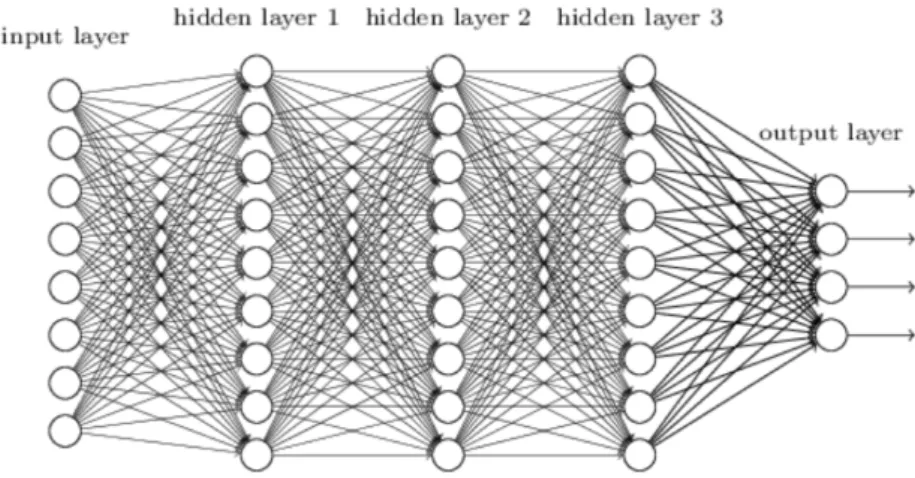
learn-Figure 2.1: An example of deep feed forward neural network

ing consists of a set of methods in which a machine is supposed to take raw data as input and automatically learn the features necessary to perform the detection or the classification. Deep Learning methods are represen-tation learning methods with multiple levels of represenrepresen-tation obtained by composing simple but non linear modules such that the complexity of the obtained representation increases with the number of levels designed. The term deep learning identifies computational models that are composed of multiple transformation layers able to learn representations of data with multiple levels of abstraction. Deep learning methods aim at automati-cally learn high-level features hierarchies by combining lower level features. Automatically learning features at multiple levels of abstraction allows a system to learn very complex functions that map the input to the output directly from data itself, without using human hand-crafted features [42]. Deep learning models are based on deep feedforward neural networks. In the following sections a general description of feedforward neural networks is given, for then focusing on convolutional neural networks, a particular kind of neural networks specifically designed to work with images.

2.1 Deep Feedforward Neural Networks

The aim of a feed forward networks is to approximate some function y = f (x) that, in the case of a classifier, maps an input x to a category y. A feedforward network determines a mapping y = f (x; θ) and learns the value of the parameters θ that results in the best function approximation [45]. These models are called feedforward because there are no feedback connec-tions between the units, which means that the information flows through the function being evaluated from x, through the intermediate computations used to determine f , and finally to the output y. Deep feedforward neural networks are considered the basis of many machine learning applications. This kind of models are mathematically based on the composition of many

(35)

2.1 Deep Feedforward Neural Networks

different functions, building the final f (x), according to a chain structure.

Let us suppose to combine three functions f(1)_{, f}(2)_{, f}(3) _{in a chain}

struc-ture, to form f (x) = f(3)(f(2)(f(1)(x))). In this model, f(1) is defined as the

first layer of the network, f(2) _{is the second layer, and so on. The overall}

length chain represents the depth of the model and in general the terminol-ogy “deep learning” derives from this structure. The final layer of a feed forward neural network is called the output layer. During the training of

the neural network the evaluated function f (x) is supposed to match f∗(x).

Each sample x provides a label y ≈ f∗(x). The training examples specify

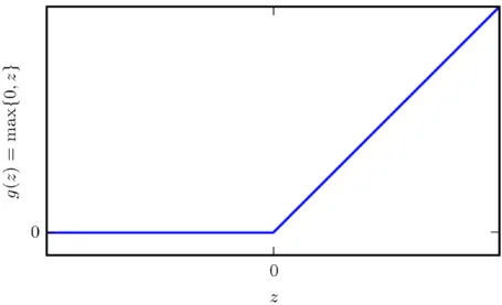
directly what the output layer must do at each point x: it must produce an output value that is as closest as possible to y. However, the training data does not show the desired output for each layer interposed between the input layer and the output layer. For this reason these intermediate layer are called hidden layers (see Fig. 2.1). Finally, these networks are defined neural because they are inspired to brain neural networks. Each hidden layer is made up of many units, acting in parallel, which are supposed to resemble brain neurons since they receive input from many other units and calculate its own activation value [45]. Now it is important to understand the importance of the activation functions that are used to compute the hidden layers values. In modern neural networks the recommendation is to use the Rectified Linear Unit (ReLU) [46], defined by the function

g(z) = max {0, z} (2.1)

depicted in Fig. 2.2. Applying this function to the output of a linear trans-formation gives a non-linear transtrans-formation. The function remains very similar to a linear function, with the main difference that a rectified linear unit outputs zero across half of its domain. This makes ReLU preserv-ing many of the properties that make linear models easy to optimize with gradient-based methods that will be discussed later. Typically, Rectified Linear Units are used on top of an affine transformation in this way:

f = g(WTx + b) (2.2)

The learning process of a deep feedforward neural network learns the weights that express the importance of the respective inputs to the output. The aim is to develop a learning algorithm able to find weights and biases so that the output from the network approximates the actual value for all training inputs to be classified.

2.1.1 Gradient-based Learning: Stochastic Gradient

Descent

The training procedure of a deep feedforward neural network consists of an iterative propagation of samples through the network and modification of its weights, which are properly initialized [47]. Deep neural networks are trained using the back-propagation algorithm by minimizing a given objective function, cost function or loss function with respect to the weights w. For a dataset D, the optimization objective is the average loss over all |D| data instances: L(w) = 1 |D| |D| X i=1 fw(x(i)) (2.3)

(36)

Figure 2.2: ReLu activation function

Since D can be very large, a stochastic approximation of this objective is used, where the cost over the entire training set is approximated with the cost over mini-batches of data. Drawing a mini-batch of N << |D| instances the optimization function becomes:

L(w) ≈ 1 |N | |N | X i=1 fw(x(i)) (2.4)

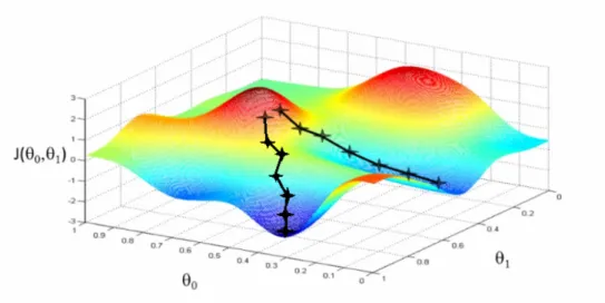
The gradient of a function generalizes the notion of derivative to the case of functions with multiple inputs. Local and global minima of the loss function can be found by moving in the direction of the negative gradient. This is known as the gradient descent method. Training a neural network consists in training the model with gradient descent. Nearly all of deep learning architectures, and also deep feedforward neural networks, are trained using an extension of the gradient descent algorithm: the Stochastic gradient descent (SGD).

The stochastic gradient descent updates the weights w by a linear

com-bination of the negative gradient ∇Lw and the previous weight update Vt

according to the following formula:

Vt+1 = µVt− α∇L(wt) (2.5)

where α and µ are two hyperparameters that are chosen for the learning procedure.

2.1.2 Learning rate

The coefficient α is called the learning rate and controls the size of the weight updates (see Fig. 2.3) A too high learning rate will make the learn-ing jump over minima, but a too low learnlearn-ing rate will either take too

(37)

2.1 Deep Feedforward Neural Networks

Figure 2.3: Stochastic Gradient descent: the role of learning rate

long to converge or get stuck in an undesirable local minima. In order to achieve faster convergence, prevent oscillations and getting stuck in unde-sirable local minima the learning rate is often varied during training either in accordance to a learning rate schedule or by using an adaptive learning rate. Common learning rate schedules include time-based decay, step decay and exponential decay.

2.1.3 Momentum

The parameter µ is the momentum that indicates the contribution of the previous weight update in the current iteration. The momentum algorithm accumulates an exponentially decaying moving average of past gradient and

continues to move in their direction as shown in Fig. 2.4 by determining

how quickly the contributions of previous gradients exponentially decay [45].

2.1.4 Dropout

When training a network with a large number of parameters, an effective regularization mechanism is essential to prevent overfitting. Regularization consists in adding a penalty on the different parameters of the model to reduce the freedom of the model itself and hence reducing probability of fitting the data noise. Classical regularizers such as L1 or L2 regularization have been found to be insufficient in this context. Dropout is a powerful regularization method [48] which has been shown to improve generalization for large neural nets. With dropout, a subset p of network units is drawn at random and temporarily “switched off” during training 2.5. When in this state, those units do not propagate signals when a sample is presented, nor participate in the process of error backpropagation. As a result, only a random subset of neurons are trained in a single iteration of SGD by forcing the neural network to learn more robust features that are useful

(38)

Figure 2.4: Stochastic Gradient descent: the role of momentum

in conjunction with many different random subsets of the other neurons. At test time, all neurons are used, and the activation of each neuron is multiplied by p to account for the scaling.

2.2 Convolutional Neural Networks

Convolutional Neural Networks (CNNs) [49] are a particular kind of deep neural networks well suited to work with images as they directly take in input 2D or 3D structures, preserving configuration information of the data. CNNs are based on three main architectural ideas: local receptive fields, weight sharing, and subsampling in the spatial domain. A typical CNN principally consists of three types of layers: (i) convolutional layers, (ii) sub-sampling layers, and (iii) output layers, that are arranged in a feed-forward structure [42] (see Fig. 2.6).

2.2.1 Convolutional layers

Convolutional layers are responsible for detecting local features in all loca-tions of the input images. To detect local structures, each node in a con-volutional layer is connected to only a small subset of spatially connected neurons in the input image channels, called receptive field. Furthermore, to enable the search for the same local feature, connection weights are shared between all the nodes in the convolutional layers; each set of shared weights is called convolutional kernel. For each convolutional layer, a set of

convolu-tional kernels W = {W1, W2, . . . , Wn} is convolved with the input image X,

(39)

2.2 Convolutional Neural Networks

Figure 2.5: Comparison between a standard deep neural network and the same network with dropout application. The circles with a cross symbol inside denote deactivated units.

map Xi through an element-wise non-linear transform σ:

Xi = σ(Wi∗ X + bi) ∀i = 1, . . . , n (2.6)

Due to the local connectivity and weight sharing, the number of param-eters compared to a fully connected neural network are greatly reduced, and thus it is possible to avoid overfitting. Further, when the input image is shifted, the activation of the units in the feature maps is also shifted by the same amount, which allows a CNN to be equivariant to small shifts, as

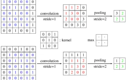
illustrated in Fig. 2.7. In the figure, when the pixel values in the input

image are shifted by one-pixel right and one-pixel down, the outputs after convolution are also shifted by one-pixel right and one-pixel down.

2.2.2 Max pooling layers

Each sequence of convolutional layers is followed by max pooling layers, that are applied to reduce the size of feature maps by selecting the maximum value in local neighbourhoods. Specifically, each feature map in a pooling layer is linked with a feature map in the convolution layer, and each unit in a feature map of the pooling layer is computed based on a subset of units in its receptive field. Similar to the convolution layer, the receptive field that finds a maximal value among the units in its receptive field is convolved with the convolution map but with a stride of the size of the receptive field so that the contiguous receptive fields are not overlapped. The role of the pooling layer is to progressively reduce the spatial size of the feature maps, and thus reduce the number of parameters and computation involved in the network. Another important function of the pooling layer is for translation invariance over small spatial shifts in the input. In Fig. 2.7, while the bottom leftmost image is a translated version of the top leftmost image by one-pixel right and one-pixel down, their outputs after convolution and pooling operations are the same (see units in green).

(40)

Figure 2.6: Convolutional neural network with two convolutional layers, one pooling layer and one dense layer. The activations of the last layer are the output of the network.

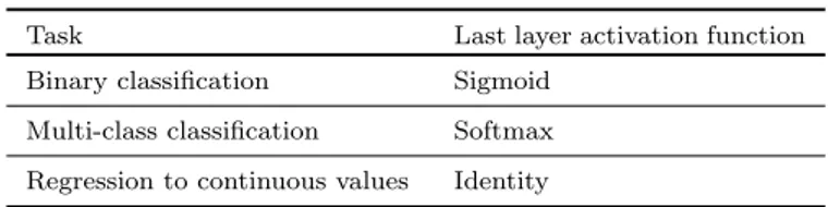
Table 2.1: A list of commonly applied last layer activation functions for various tasks

Task Last layer activation function Binary classification Sigmoid

Multi-class classification Softmax Regression to continuous values Identity

2.2.3 Fully connected layers

At the end of the convolutional stream of the network, a number of con-secutive fully connected layers is added, and the class distribution over the classes is generated by feeding them through an activation function. Neu-rons in a fully connected layer have connections to all activations in the previous layer, as in regular non-convolutional artificial neural networks 2.1. Their activations can thus be computed as an affine transformation, with matrix multiplication followed by a bias offset.

Last layer activation function

The activation function applied to the last fully connected layer is usually different from the others. An appropriate activation function needs to be selected according to each task. An activation function applied to the mul-ticlass classification task is a softmax function which normalizes outputs of the last fully connected layer to target class probabilities, where each value ranges between 0 and 1 and all values sum to 1. Typical choices of the last layer activation function for various types of tasks are summarized in Table 2.1.

(41)

2.3 Deep CNN architectures

Figure 2.7: Illustration of translation invariance in convolutional neural network. The bottom leftmost input is a translated version of the upper leftmost input image by one-pixel right and one-pixel down.

2.3 Deep CNN architectures

When architecting a CNN for a particular task there are multiple factors to consider, including understanding the task to be solved and the require-ments to be met and optimize computation and memory footprint. In the early days of modern deep learning it was common to use very simple com-binations of the building blocks. Later on, network architectures became much more complex, resulting in updates to the state-of-the-art. In this section a general overview about the best-known CNN network architec-tures is given, with a particular focus on the ones that are commonly used for medical image tasks, i.e medical image classification and segmentation.

2.3.1 Classification architectures

LeNet [49] and AlexNet [50], introduced over a decade ago, were the very first convolutional architecture to be proposed, being in essence very sim-ilar models. Both networks were relatively shallow, consisting of two and five convolutional layers, respectively, and employed kernels with large re-ceptive fields in layers close to the input and smaller kernels closer to the output. AlexNet did incorporate rectified linear units instead of the hy-perbolic tangent as activation function, which are now the most common choice in CNNs. After 2012 the exploration of novel architectures took off, and in the last years there is a preference for far deeper models. By stack-ing smaller kernels, instead of usstack-ing a sstack-ingle layer of kernels with a large receptive field, a similar function can be represented with less parameters. This approach ensures the same effective receptive field, by increasing at the same time the number of non-linearities (which makes the decision function more discriminative) and decreasing the number of parameters. Simonyan et al.[51] were among the first to explore much deeper networks, and

Deep Learning for computer-aided detection and diagnosis of clustered microcalcifications on digital mammograms

UNIVERSITÀ DEGLI STUDI DI

CASSINO E DEL LAZIO MERIDIONALE

Corso di Dottorato in

Metodi modelli e tecnologie per l’Ingegneria

Ciclo XXXII

Deep Learning for computer-aided detection and diagnosis of

clustered microcalcifications on digital mammograms

accompagnato in questo meraviglioso percorso di

vita...

Abstract

Contents

List of Figures

List of Tables

Chapter 1

Introduction

1.1

Anatomy of the breast

(c)

(d)

(b)

(a)

(a)

(b)

I

II

III

1.2

Malignant breast diseases

1.3

Breast imaging

1.3.1

Mammography

1.3.2

Screen-film mammography

1.3.3

Full-field digital mammography

(a)

(b)

1.4

Signs of breast cancer in mammography

1.4.1

Microcalcifications

1.4.2

Soft tissue lesions

1.5

Computer aided detection and diagnosis

1.6

Evaluation of CAD

1.7

Outline of the thesis

Chapter 2

Deep Learning

2.1

Deep Feedforward Neural Networks

2.1.1

Gradient-based Learning: Stochastic Gradient

Descent

2.1.2

Learning rate

2.1.3

Momentum

2.1.4

Dropout

2.2

Convolutional Neural Networks

2.2.1

Convolutional layers

2.2.2

Max pooling layers

2.2.3

Fully connected layers

2.3

Deep CNN architectures

2.3.1

Classification architectures