ESSAYS IN PUBLIC ECONOMICS AND POLICY

I

Università degli Studi di Messina

Phd programme in

Economics, management and statistics

XXX cycle

ESSAYS IN PUBLIC ECONOMICS

AND POLICY

S.D.D. SECS-P/03

Phd thesis by

Francesca Nordi

Supervisors

Prof. Giuseppe Migali

Prof. Leonzio Giuseppe Rizzo

Prof. De Benedetto

I

Contents

Preliminary note

Chapter 1:

Spatial interaction in local expenditures among Italian

municipalities: evidence from Italy 2001-2011

1.1 Introduction

1.2 Institutional framework: a brief analysis of Italian

municipalities’ spending

1.3 Empirical framework

1.4 Data

1.4.1 Dependent variables and variables of interest.

1.4.2 Control variables

1.5. Results

1.6. Robustness tests

1.6.1 Different weighting matrices

1.6.2 An experimental setting

1.7. Testing for sources of spatial interdependence

1.7.1 Yardstick competition hypothesis

1.7.2 Spillover Hypothesis and the size of municipalities

1.8 Conclusion

1.9 Appendix

1.10 References

Chapter 2: The political budget cycle of EU Funds’ spending

process: Evidence from Italian municipalities.

2.1 Introduction

2.2 The design of Structural Funds Allocation through Italian

municipalities

2.3 Brief literature review of EU structural funds

2.4 The political budget cycle

2.5 Dataset and variables

2.5.1 Dependent variables

2.6 Empirical analysis and results

2.6.1 Estimation results - Dataset 1 – LAUNCH date project year

2.6.2 Estimation results - Dataset 2 – END date project year

II

2.7 Conclusion

2.8 Appendix

2.9 References

Chapter 3: The employment protection legislation in Italy: different

restricted firms’ reaction to a tax rate cut

3.1 Introduction

3.2 Institutional background

3.3 Theoretical consideration on EPL and empirical studies

3.3.1 EPL and profitability

3.4 Empirical analysis

3.4.1 Dataset, sample selection and preliminary evidence

3.4.2 Identification strategy and regression model

3.4.3 Profitability and employment level variation

3.4.4 Robustness tests

3.5 Conclusion

3.6 Appendix

1

Preliminary note

This dissertation is composed of three autonomous chapters that empirically investigate issues related to public economics exploiting micro level data. Chapter 1 and chapter 2 evaluate spending and political behavior of Italian local institutions, Chapter 3, instead, concentrates on firms’ profitability and employment level. A common ground in all the three chapters is the effort to identify conditions that enable to estimate “causal effects”. In particular, in the first analysis I estimate the effect of neighboring municipalities’ spending on municipality. The second chapter focuses on the effect of Political budget cycle on the European structural funds’ municipal utilization. The third chapter investigates the effect of Employment legislation constraints on firms’ profitability and employment level.

As exemplified in Angrist, J.D., Pischke, J.S. (2009) the causal effect is “what would happen to a given individual not hospitalized in a hypothetical comparison of alternative hospitalization (scenarios)”; in order to identify the effect of a scenario on the individual we have to compare it to the effect on individual in the opposite situation. The problem is that we cannot observe the individual in the two scenarios because only one realized. In presence of randomization the selection problem is avoided, such as for experiments in medicine when is random if an individual experiment the scenario 1 or the opposite one. If we are not in presence of randomization, we have to solve the problem of lack of information, facing with the concept of “counterfactual” (Loi, M. and Rodrigues, M.,2012). A counterfactual is for the individual in the happened scenario the potential outcome for the alternative state, and for the individual that do not experiment the scenario the potential outcome if they would be experimented it. When we think to this type of analysis the framework is always composed by a part of the population or of the sample which is subjected to the treatment. The researcher’s effort consists on finding a reliable control group. In fact, it is not always available or it is not easy to identify a reliable one that is not affected by the selection bias, a type of distortion for which an individual belongs to a group which receive a treatment or experiment a scenario because of its characteristics and not randomly assigned. The econometric theory formulates techniques to construct an adequate control group, this process is known as identification strategy and consent to simulate the counterfactual outcome, solving the problem of selection bias. These identification strategies allow us identifying the causal effect; in absence of this identification, we can only talk about correlation between the treatment (scenario) and the outcome.

Chapter 1 explores the existence of spatial effect on Italian municipalities’ spending decisions. I estimate a spatial autoregressive dynamic panel data model, using information on 5,564 Italian municipalities over the period 2001-2011, exploiting their border contiguity as a measure of spatial neighborhood. I find a positive and statistically significant effect of neighboring expenditures on total, capital and current expenditures of

2

a given municipality. These results are robust to the use of alternative weighting matrices for the definition of spatial neighbors. Anyway, this type of analysis, within the framework of spatial econometrics that use internal instruments, does not offer, in general, a valid identification of causal relation, and in turn, might lead to biased estimates. For this reason, I also employ a quasi-natural experimental approach to estimate a causal effect. The randomization of the data can not be exploited, for this reason it is necessary taking advantage of a particular condition in the observable data which enables to set up a quasi-natural experiment. In my case I exploit the exogenous variation in the neighbors’ spending induced by the devastating earthquake occurred in 2009 in Abruzzo. The natural event hits municipalities belonging to the L’Aquila area, but not all municipalities of Abruzzo region. I can identify a group hit by the earthquake, whose average expenditure increased with the earthquake intensity. In this way, the new instrument used in the analysis is based on an unexpected natural disaster and it is reasonable to consider it as exogenous for any single municipality. The results confirm the presence of interdependence between municipalities’ spending. Moreover, I do not find any evidence of yardstick competition when I take into account political effects, while I do find a negative relationship between spatial interaction and the size of the municipality. Thus, I conclude that spillover effects drive the strategic interactions in spending decisions among Italian municipalities.

Chapter 2 focuses on the dynamic of the European Structural funds’ utilization at municipal level. I investigate the presence of Political Budget Cycle (PBC) demonstrating that mayors exploit the possibility to implement projects in their territory in order to send out a signal for the electorate. I estimate the existence of a causal relationship between PBC and the probability to start or end at least one EU projects, between PBC and the number of projects started or ended and between PBC and fragmentation of the EU projects realized. I use information on 3,102 Italian municipalities over the period 2007-2014, also distinguishing between municipalities of Convergence objective regions and

Competition and employment objective regions (objective’s European classification for

EU Structural Funds). In this case the causal relationship between the variables tested is assured by the randomly assignment distribution of the dummy independent variable PBC equal to 1 if the year is the year before the election. The year of election, and consequently the year before the election, cannot be modified by the mayors and depends on a historical dynamic at national level and it does not depend on the characteristics of municipalities. We can say that belonging to the group of municipalities going to election in a particular year is random. I find evidence of the existence of PBC in the dynamic of EU structural funds’ process, with differences related to the nature of projects realized linked to EU Objectives.

Finally, Chapter 3 concentrates on firm level data, trying to identify a causal effect through an experimental econometric approach. I test the effect of the Employment Protection Legislation on Italian firms’ performance and on the level of employment. I use a panel dataset at firm-level for the period 2005-2011 which contains data of corporations. I set up an identification strategy based on a discontinuity regression design and a

difference-3

in-differences approach, even with an unconventional use of the dummy variable pre and post. I exploit the discontinuity on EPL at the 15 employees’ threshold for Italian firms, established by the Articolo 18 of the Statuto dei lavoratori (law n. 300/1970), that set different level of regulations for firms above the limit of 15 employees and below this limit. I also exploit a tax rate cut occurred in 2008 (the Ires tax) to fix a pre and a post period, to test the reaction of these group of firms in term of profitability and employment level to a decreasing in taxation. I find a negative and statistically significant effect of EPL on profitability, measured by Roe and Roa, and on the level of employment. Firms less constraints by EPL, below the limit of 15 employees, show a positive reaction to the tax rate cut if compared to the firms above the limit of 15 employees.

Key words: Local public spending interactions, spillovers, yardstick competition,

Political business cycles; European structural funds; local governments Employment protection legislation, firms, profitability, employment

JEL codes: C23, H72

References

Angrist, J.D., Pischke, J.S. (2009). “Mostly Harmless Econometrics: An Empiricist's Companion”, Princeton University Press

Loi, M. and Rodrigues, M. (2012). “A note on the impact evaluation of public policies: the counterfactual analysis”, Joint Research Centre, European Commission

4

Chapter 1

Spatial interaction in local expenditures among Italian

municipalities: evidence from Italy 2001-2011

Abstract

I estimate a spatial autoregressive dynamic panel data model, using information on 5,564 Italian municipalities over the period 2001-2011, exploiting their border contiguity as a measure of spatial neighborhood. I find a positive and statistically significant effect of neighboring expenditures on total, capital and current expenditures of a given municipality. These results are robust to the use of alternative weighting matrices for the definition of spatial neighbors and also when I employ a quasi-natural experimental approach, which exploits the exogenous variation in the neighbors’ spending induced by the devastating earthquake that in 2009 hit municipalities belonging to the Abruzzo region. Moreover, I do not find any evidence of yardstick competition when I take into account political effects, while I do find a negative relationship between spatial interaction and the size of the municipality. Thus, I conclude that spillover effects drive the strategic interactions in spending decisions among Italian municipalities.

Key words: Local public spending interactions, spillovers, yardstick competition,

5

1.1 Introduction

Many studies in the last two decades aimed to assess the existence of spatial effects influencing local expenditure decisions. In particular, there is a line of works1, both theoretical and empirical, that investigates whether governments make their spending decisions by taking into account the behavior of their neighbors. In such a framework, decisions on expenditures would depend not only on the traditional determinants of local spending, such as income, grants, socio-demographic and political characteristics of municipalities, but also on spending decision of neighboring municipalities. Indeed, if municipalities choose their expenditures/taxes – which can affect the welfare of their neighbor’s – by maximizing their own welfare and so not taking into account their neighbor’s welfare, they end up into inefficient levels of expenditure and/or taxes (Gordon, 1983).

The existence of strategic interactions between local governments is theoretically explained by several models, e.g. yardstick competition, tax and welfare competition, spillover effects and, more recently, political trend models. In the yardstick competition model, voters with no complete information on the cost of public goods and services compare expenditures and taxes in their jurisdiction with those of nearby jurisdictions (Salomon, 1987) and, hence, voters punish the incumbent politician if her tax rate decisions are not in line with those of neighbors. Starting from the seminal work of Besley and Case (1995) – who show that neighbors’ tax rates impact on the probability of re-election for the incumbent in US states – a substantial body of literature has developed documenting and empirically testing yardstick competition (see, among others, Revelli, 2002a; Bordignon et al., 2003; Solé-Ollé, 2003; Allers and Elhrost, 2005; Padovano and Petrarca, 2014). The second source of spatial interdependence arises in tax competition models. Municipalities face mobile tax bases, which depend on both their own tax rate and their neighbors’ tax rate giving rise to tax competition (Kanbur and Keen, 1993; Devereux et al., 2008; Rizzo, 2008). As far as the traditional “spillover” model is concerned, public expenditures of a municipality may have positive or negative effects beyond its own boundary, thus affecting the welfare of residents in neighboring municipalities. As a result, municipalities might decide the level of their own expenditure, by strategically taking into account the expenditures of their neighbors (Case et al 1993; Revelli, 2002b; Revelli, 2003; Baicker, 2005; Solé-Ollé, 2003; Werck et al., 2008; Costa et al., 2015). Finally, strategic interactions among local governments can be also explained by political interactions. This idea is based on the assumption that the local incumbent politician, taking into account the common ideology, makes her decisions on taxes and expenditure by looking only to those neighbors belonging to the same political party (Geys and Vermier, 2008; Santolini, 2009). Empirical findings support this hypothesis. In particular, Foucault et al., (2008), by using a panel data-set on French municipalities over

1 _{For a theoretical survey on horizontal strategic interaction see, for example, Wilson (1999), while for an empirical survey on fiscal}

6

the period 1983-2002, show that spending interactions exist between municipalities that have the same political affiliation. The same results are confirmed for Spanish municipalities by Delgado et al., (2014), while for the Italian case, political ideology is a relevant determinant of fiscal interaction only for right-wing and centrist parties (Santolini, 2008)2.

Most of the empirical literature estimates fiscal strategic interactions by considering the tax side of the local budget. Indeed, there are only few papers that focus explicitly on public expenditures (Case et al., 1993; Figlio et al., 1999; Baicker, 2005; Revelli 2002 and 2003, Foucault et al., 2008 and Costa et al., 2015) and, among these, only two works deal with the Italian framework (Ermini and Santolini, 2011; Bartolini and Santolini, 2012). However, these studies are conducted on sample of sub-national Italian jurisdictions (municipalities belonging to Marche region3) and they focus only on current expenditure, so that, at the best of my knowledge, no one has investigated strategic interactions in both current and capital expenditure decisions, by using a comprehensive dataset on Italian municipalities.

In this work, I aim to fill this gap by assessing the existence of spatial effects influencing the spending decisions of Italian municipalities and identifying the source of such interdependences. I use information on all Italian municipalities (except for those in autonomous regions) over the period 2001-2011. By employing the Arellano-Bond estimator; I estimate an empirical model where the public expenditure in a given municipality depends on the average of their own border municipalities’ expenditures and on a set of control variables, including the lagged value of expenditure. I find a positive horizontal interdependence in spending decisions among Italian municipalities. However, some political variables turn out to be important determinants of local expenditure. In fact, the election year positively affects both total and capital expenditure, implying the presence of the political budget cycle among Italian municipalities. Moreover, the level of expenditure is higher among those municipalities where the mayor wins the election with a strong majority. Interestingly, I also find that the population size of the municipality negatively affects the impact of neighbors’ expenditure on its own expenditure, such that, above a certain population level, the positive horizontal interdependence in the municipal expenditure vanishes. This last finding together with the no significant interactions with political variables (i.e., electoral and pre-electoral years, the political power of the mayor and mayors that, according to the Italian law, cannot be re-elected) let me argue that the strategic interaction is due to spillover effects and it is not driven by yardstick competition.

2 _{The role of political ideology has been found to be an important driver also at the country level, as shown by Cassette and Exbrayat}

(2009), who conduct an analysis on 27 European countries over the period 1995-2007 finding that ideology on tax interactions holds only for contiguous countries.

3 _{Ermini and Santolini (2011) found a positive and significant spillover effect for current expenditure, while, Bartolini and Santolini}

7

The main contribution of this paper derives from the properties of the dataset. Since it includes all Italian municipalities for the period 2001-2011, it allows testing the existence of local spending interactions by also controlling for the persistency in local expenditures. Such a feature has been exploited only by few papers, including Foucault at al. (2008); Bartolini and Santolini (2012) and Costa et al. (2015)4. Moreover, this study is the first that investigate the source of interactions on capital expenditure for the Italian case. The local policy maker uses these investments as a way to attract economic activities, firms and households, and hence it is highly likely to observe strategic interactions between municipalities: if two municipalities are neighboring and one of them invests in roads, there is an incentive also for the other municipality to invest in roads, as the benefits from road usage are expected to be higher for the residents of the two municipalities if roads are provided on both jurisdictions than in the case in which only one jurisdiction provides good roads. Finally, I test the robustness of my results not only by using alternative weighting matrices - as it is common in the applied literature of spatial econometrics -, but also by employing a quasi-natural experimental approach. In particular, I focus on the period 2009-2010, since 49 municipalities of Abruzzo region were hit in year 2009 by a dreadful earthquake that caused economic losses of more than 14.7 billion euros. I thus build a dummy variable equals to one for municipalities hit by the earthquake, and then I convert it in a measure of the intensity of the earthquake by using the Mercalli-Carcani-Sieberge scale. The neighbors' value of this variable is then used to instrument the change in the average expenditure of neighboring municipalities from 2009 to 2010. The estimates of spatial interactions in municipal expenditure obtained in this experimental context confirm those obtained by relying on internal instruments (using the same sample of municipalities belonging to Abruzzo region), and so pointing to the existence of interactions in public expenditure among local governments.

The rest of paper is organized as follows: Section 1.2 illustrates the institutional framework; Section 1.3 discusses the econometric strategy and Section 1.4 describes the data. Section 1.5 presents the main results, while robustness tests are shown in Section 1.6. Then, in Section 1.7, I investigate more in depth the source of spatial interaction, by testing yardstick competition and spillover hypotheses. Finally, Section 1.8 concludes.

4 _{It is worth noting that the dataset includes 61,204 observations, making it the largest sample ever examined in applied work on}

strategic interactions in spending decisions at the local level. In fact, among those papers analyzing the existence of interactions related to public expenditure, Foucault at al., (2008) use a panel dataset of 90 French municipalities over the period 1983-2002, leading to 1,710 observations; Bartolini and Santolini (2011) rely on a panel dataset of 246 Italian municipalities of Marche region during the period 1994-2003, for a total of 2,460 observations and Costa et al., (2015) use a panel dataset of 278 Portuguese municipalities for the period 1986-2006, summing up to 5,560 observations.

8

1.2 Institutional framework: a brief analysis of Italian municipalities’

spending

The Italian Constitution defines four administrative government layers: central government, regions, provinces and municipalities. While most regions and provinces are ruled by ordinary statutes, some of them – the autonomous regions and provinces – are ruled by special statutes5. Furthermore, Italy counts 110 provinces, that have recently been reformed by the law 56/2014, which reduced their public competences and eliminated the possibility of direct elections of their own representatives. Finally, municipalities are the smallest level of jurisdiction and are around 8,000, although this number is decreasing because the law 56/2014 is incentivizing amalgamation. Most municipalities (around 90%) have less than 15,000 inhabitants and the average size is around 6,400 inhabitants. Municipalities in Italy are responsible for several public functions, such as social welfare services, territorial development, local transport, infant school education, sports and cultural facilities, local police services, water delivery, rubbish as well as most infrastructural spending. According to the data, municipalities’ total expenditure accounts, on average, for about 8.7% of all total public expenditure in Italy during the period 2001-2011.

Municipalities’ current expenditure, on average, accounts for 71% of the municipalities’ total expenditure, which corresponds to 63 billion of euros per year during 2001-2011. Among current expenditure, approximately 75% is concentrated on four main functions:

Administration and Management, Roads & Transport Services, Planning and Environment and Social welfare. The remaining 25% of the current expenditure is

allocated to the Municipal police, Education, Culture, Sport, and Tourism. Finally, a very low amount of resources goes to three functions, Economic development, In-house

production services and Justice, managed by many medium-sized and small

municipalities networking with other municipalities.

Municipalities are also responsible for investments, which are on average 29% of the total expenditure in the period 2001-2011. However, it is worth noting that the share of these expenditures sharply decreased in the period 2006-2011, switching from 34% to 21% of total expenditures. At the same time, the share of current expenditure has increased. Looking at the specific functions, municipalities allocate resources for investments mainly to Administration and Management (16.7% of the capital expenditure) Roads and

Transport Services (26%), Planning and Environment (27.5%) and Education (9%).

5 _{In Italy there are five autonomous regions (Sicilia and Sardegna, which are insular territories, and Valle d’Aosta, Trentino Alto Adige}

9

1.3 Empirical framework

The econometric strategy is based on the estimation of a spatial autoregressive dynamic panel model (Anselin et al., 2008), which takes the following form:

𝐺_𝑖𝑡 = 𝛼 + 𝛽𝐺_{(𝑖𝑡−1)}+ 𝛾𝑊𝐺_−𝑖𝑡+ 𝜌𝑋_𝑖𝑡+ 𝜇_𝑖 + 𝜏_𝑡+ 𝜀_𝑖𝑡, (1) where 𝐺_𝑖𝑡 is the per capita expenditure of municipality i in year t, and 𝐺_{(𝑖𝑡−1)} is its one year lagged value.

𝑊𝐺−𝑖,𝑡= ∑𝑗≠𝑖𝜔𝑖𝑗𝐺𝑗𝑡 is the weighted per capita average expenditure of the neighboring

municipalities j at time t; ω_ij are exogenously chosen weights that aggregate the per capita expenditure of neighboring municipalities into a single variable WG_−i,t. The ω_ij are normalized so that ∑_j≠iω_ij = 1. 𝑋_𝑖𝑡 is a matrix of demographic, socio-economic and political characteristics of municipality i at time t, and it also includes per capita transfers (current, capital or total grants, according to the dependent variable adopted in the estimation) from upper tiers of governments (𝑡𝑟𝑎𝑛𝑠𝑓𝑒𝑟𝑠_𝑖𝑡).6 μi is an unobserved

municipal specific effect, τt is a year specific intercept and εit is a mean zero, normally

distributed random error.

In equation (1), the coefficient β measures the degree of inertia of the municipal expenditure, whereas the coefficient γ captures the horizontal interdependence in the municipal expenditure, that is the reaction of the expenditure of a given municipality to a one-euro increase in the average expenditure of its neighbors. The interpretation of the coefficient γ, as capturing the horizontal interdependence in the municipal expenditure, is very common in the literature (see, among others, Foucault et al., 2008; and Costa et al., 2015, who explicitly interpret it as a spillover effect). As far as the spillover effect is concerned, there are three possible cases, which are related to the degree of complementarity and substitutability in the provision of public goods and/or services:

i) γ =0: no horizontal interdependence, namely municipalities do not imitate each other in setting local public spending.

ii) γ< 0: negative horizontal interdependence, that is a one-euro increase in the average expenditure of neighboring municipalities leads to a reduction in the municipal expenditure. This case holds when public goods/services provided by neighbors’ municipalities are substitutes of the municipality’s own goods/services. For example, two swimming pools, one located in each municipality, are likely to be substitutes and, hence, there is no incentive for a given municipality to increase its expenditure as a response to an increase in neighbors’ expenditure.

iii) γ> 0: positive horizontal interdependence, that is a one-euro increase in the average expenditure of neighboring municipalities leads to an increase in the

6 _{In the years 2008-2011 we subtract the compensative transfer from the central state that has been introduced to replace the missing}

10

municipal expenditure. This case holds when public goods/services provided by neighbors’ municipalities are complements of the municipality’s own goods/services. For example, road services provided by the two municipalities are likely to be complements and, hence, there might be an incentive for a given municipality to increase its expenditure as a response to an increase in neighbors’ expenditure.

Since equation (1) includes endogenous variables, the OLS estimation is inappropriate as it generates biased estimates. The average neighboring expenditure, 𝑊𝐺_−𝑖𝑡, is endogenous because expenditure interactions are symmetric and simultaneous: each municipalities’ behavior affects that of its neighbors and it is affected by their behavior in the same way. The lagged dependent variable, 𝐺(𝑖𝑡−1), which is an important determinant of the

municipal expenditure (Veiga and Veiga, 2007; Larcinese et al., 2013), is correlated with the municipality fixed effects in the error term, leading to biased and inconsistent fixed effects estimations (Nickell, 1981). The variable 𝑡𝑟𝑎𝑛𝑠𝑓𝑒𝑟𝑠𝑖𝑡 is also endogenous, as

simultaneously decided with municipalities’ expenditures. Thus, I use the system GMM (SYS-GMM) dynamic panel estimator (Arellano and Bover,1995; Blundell and Bond, 1998).

This estimator is an augmented version of the difference GMM (Arellano and Bond, 1991) and, hence, is considered more efficient with respect to the difference GMM (Blundell and Bond, 1998). The SYS-GMM, differently from the difference GMM which just employs the difference equation, builds a stacked dataset, one in levels and one in differences. Then the differences equations are instrumented with levels, while the levels equations are instrumented with differences7.

The consistency of the GMM estimator depends on the assumption that the error term is serially uncorrelated, otherwise the instruments are not valid. Hence, to check for the absence of first-order serial correlation in levels in a dataset expressed in differences, as that used in a SYS-GMM, I need to check for the absence of second order correlation in differences. In fact, I am able to detect first order serial correlation in level between 𝜀_𝑖𝑡−1 and 𝜀_𝑖𝑡−2 by looking at the correlation between ∆𝜀_𝑖𝑡 (∆𝜀_𝑖𝑡 = 𝜀_𝑖𝑡− 𝜀_𝑖𝑡−1) and ∆𝜀_𝑖𝑡−2 (∆𝜀_𝑖𝑡−2 = 𝜀_𝑖𝑡−2− 𝜀_𝑖𝑡−3). For this reason, I test, using the differenced estimating equation, for first order autoregressive (AR(1)) serial correlation in the residuals, which I expect negative and significant8 _{and for second order autoregressive (AR(2)) serial}

7 _{In terms of equation (1) we take the first difference, then the term 𝐺}

𝑖𝑡−1 in ∆𝐺𝑖𝑡−1 (∆𝐺𝑖𝑡−1= 𝐺𝑖𝑡−1− 𝐺𝑖𝑡−2) is correlated with the

term 𝜀𝑖𝑡−1 in ∆𝜀𝑖𝑡 (∆𝜀𝑖𝑡= 𝜀𝑖𝑡− 𝜀𝑖𝑡−1), so the choice of 𝐺𝑖𝑡−1 as instrument would bias the estimates. As a results, for the equation in

differences, we may use lagged values of 𝐺𝑖𝑡 to form instruments as long as 𝐺𝑖𝑡 is lagged two periods or more (𝐺𝑖𝑡−2, 𝐺𝑖𝑡−3 ,… ). As

concerns the level equations, the lagged endogenous variables (𝐺𝑖𝑡−1) can be instrumented with ∆𝐺𝑖𝑡−1 since it is not correlated with

𝜀𝑖𝑡. The same approach is followed for the other 2 endogenous variables, in particular ∆𝑊𝐺−𝑖𝑡 is instrumented with two (or more)

periods lags (𝑊𝐺−𝑖𝑡−2, 𝑊𝐺−𝑖𝑡−3 ,… ) and ∆𝑡𝑟𝑎𝑛𝑠𝑓𝑒𝑟𝑠𝑖𝑡 is instrumented with two (or more) periods lags (𝑡𝑟𝑎𝑛𝑠𝑓𝑒𝑟𝑠𝑖𝑡−2,

𝑡𝑟𝑎𝑛𝑠𝑓𝑒𝑟𝑠𝑖𝑡−3 ,… ).

8 _{Since ∆𝜀}

𝑖𝑡 is analytically related to ∆𝜀𝑖𝑡−1 via the term 𝜀𝑖𝑡−1, a negative first-order serial correlation is always expected in differences.

11

correlation in the residuals, which I expect not significant (Arellano and Bond, 1991), where in both tests the null hypothesis is the absence of serial correlation in the residuals.9 In order to check the validity of the instruments, I employ the standard Hansen test whose null hypothesis is the exogeneity of the corresponding instrument (or group of instruments). However, as Roodman (2009) points out, the power of the Hansen test might be weakened if the number of instruments is high. Consequently, I test the validity of a subset of instruments by using a C-test (Baum, 2006). The C-test estimates the SYS-GMM with and without a subset of instruments and uses the difference between the two respective Hansen tests distributed as a chi2 and, allowing to test the null hypothesis that the excluded instruments are valid, namely they are exogenous.

The SYS-GMM requires an additional assumption with respect to the difference GMM: the first differenced instruments for the level equations must be not correlated with the fixed effects. For this reason, I apply the C-test to the level equation and so comparing the Hansen test of this last equation with that of the SYS-GMM. The null hypothesis is that the instruments (which are taken in difference) for the level equations are valid and so the SYS-GMM is preferred to the difference GMM.

Finally, I use a two-step SYS-GMM, which makes the covariance matrix more robust to panel specific autocorrelation and heteroskedasticity, so the estimator is more efficient (Arellano and Bond, 1991; Blundell and Bond 1998). However, by using this procedure the standard errors might be severely downward biased (Roodman, 2009), hence, in order to correct the bias, I apply the correction made by Windmeijer (2005).

1.4 Data

The data on Italian municipalities used in my work result from a combination of different archives provided by the Italian Ministry of Internal Affairs, the Ministry of Economy and the Institute of National Statistics.

The data include a full range of information for the period 2001-2011 and are organized into two sections: 1) municipality financial data and 2) municipality demographic, socio-economic and electoral data, such as population size, age structure, average income of inhabitants, election years. I restrict the sample to municipalities located in ordinary statute regions. I exclude municipalities that have a specific status of metropolitan areas (law 56/2014)10, because they usually provide a wider range of services compared to other municipalities. The final sample includes 5,564 municipalities11, observed from 2001 to 2011, which generates a balanced panel data set of 61,204 observations. It is worth noting that all financial variables are expressed in 2011 real per capita value.

The Italian municipality balance sheet reports expenditures either in accrual basis or in cash basis. In this system of public accountability there is usually a gap (exceeding,

9 _{In fact E(∆𝜀}

𝑖𝑡, ∆𝜀𝑖𝑡−2)=E(𝜀𝑖𝑡− 𝜀𝑖𝑡−1) E (𝜀𝑖𝑡−2− 𝜀𝑖𝑡−3) =0.

10 _{Milano, Roma, Napoli, Torino, Bari, Firenze, Bologna, Genova, Venezia and Reggio Calabria.}

12

sometimes, more than one financial year) between the payment (registered on cash basis) and the commitment to it (registered on accrual basis). For this reason, I prefer to use the cash basis classification, since the value is reported only if the payment has effectively been made.

1.4.1 Dependent variables and variables of interest.

I estimate equation (1) using three different dependent variables: the per capita total expenditure (total expenditure), the per capita current expenditure (current expenditure) and, the per capita capital expenditure (capital expenditure). I use these aggregate measures of expenditure and not those disaggregated by functions, because many municipalities (especially the small ones) have expenditure crossing more than one function, but often registered only in one function.

To isolate the independent impact of neighboring expenditures on the expenditure of a given municipality, I use the neighbors’ expenditures variable (neigh expenditure). In order to obtain this variable, as mentioned in Section 1.3, I use a contiguity matrix, implying 𝜔𝑖𝑗 = 1/𝑚𝑖 where 𝑚𝑖 is the number of municipalities contiguous to i and 𝜔𝑖𝑗 =

0 otherwise. Hence, for each municipality i in period t, the average value of its own neighbors’ per capita expenditure is given by 𝑊𝐺_−𝑖,𝑡= ∑_𝑗≠𝑖𝜔_𝑖𝑗𝐺_𝑗𝑡.

1.4.2 Control variables

The municipality expenditure can be affected by other factors, accounting for demographic, socio-economic and electoral characteristics. In particular, I include a set of time-varying variables, which characterizes the municipality’s demographic and economic situation. I include the municipal population (population*10-4_{) and per capita}

area (area*103) - square kilometers divided by population – as these variables can capture the presence of scale economies and/or congestion effects. The proportion of citizens aged between 0 and 5 (children*103_{) and the proportion of citizens aged over 65 (aged*10}3₎

can control for some specific public needs (e.g., nursery school, nursing homes for the elderly) and hence may influence the composition of public spending.

In terms of economic and financial controls, I include the per capita personal income tax base (income*10-3_{), i.e. a proxy of per capita average income and, per capita transfers}

(current, capital or total grants) from upper tiers of governments (transfers), that vary according to the dependent variable adopted in the estimation.12 These variables should have a positive impact on expenditure. On the one side, higher levels of local expenditure

12 _{Transfers from upper level of government represent a significant part, appoximatley around 25%, of the Italian municipal financing}

system. There is a well-known literature on the effects of grants on public expenditure (see, among others, Gramlich,1977; Hines and Thaler, 1995; Gamkhar and Shaw, 2007 and Inman, 2009) usually finding that grants can stimulate government expenditures more than monetary transfers to individuals of the same amount—the so-called flypaper effect, whereby a quota of the federal money sticks to the public sector instead of being distributed to citizens.

13

might be associate with high level of local economic development (proxied by the per-capita personal income tax base) and, on the other side, an increase in the municipal revenue (proxied by transfers) should lead to an increase in expenditure.

Furthermore, following the literature (Bordignon et al, 2003; Foucault at al., 2008; Bartolini and Santolini, 2012) I use a set of political variables that may influence the local budget. In particular, I define a dummy variable (election), which, during the period 2001-2011, is equal to 1 for a given municipality in the year of election. The coefficient of this variable is expected to be positive as the incumbent might have an incentive to expand the expenditure during the election period in order to be re-elected. I then measure the political power of the mayor by using the percentage of votes that have been necessary to win an election (vote-share): the stronger the power of the local policy maker, the grater is her capacity to influence the budget. Since Italian law establishes a limit of no more than two consecutive terms in office for a mayor, I use a dummy variable (term-limit) which is equal to 1 for all the years a mayor is at her second term (and hence she cannot be re-elected) and it is equal to 0 when the mayor is at her first term: the impossibility of further re-election may significantly bias the budget-related decisions of a municipality.

Since 200113, the Italian central government – in order to fulfill the obligations of the European Stability and Growth Pact – imposes to each municipality above 5,000 inhabitants the so-called Domestic Stability Pact. Depending on the year, it implies either a constrained municipal deficit or a threshold on the municipal expenditure. Hence, I include a dummy (domestic stability pact) equal to one if a municipality has to fulfill the Domestic Stability Pact (i.e. it has more than 5,000 inhabitants) and 0 otherwise: this variable should lead to lower level of expenditure. The summary statistics of all the variables used in the analysis are reported in Table 1.

As discussed in section 1.3, the dynamic model I estimate includes the lagged endogenous dependent variable, 𝐺_{(𝑖𝑡−1)} and two further endogenous variables, namely the average neighboring expenditure, WG−it, and per capita transfers (current, capital or total grants)

from upper tiers of governments (𝑡𝑟𝑎𝑛𝑠𝑓𝑒𝑟𝑠𝑖𝑡). Therefore, all these variables are

instrumented by using their lags14.

13 _{See law 388/2000, article 53.}

14

Table 1: Summary statistics

Variable Obs Mean Std. Dev. Min Max

Total expenditure 61,204 1251.95 1101.98 30.17 43906.23 WTotal expenditure 61,204 1226.65 719.84 0.00 15280.65 Current expenditure 61,204 742.04 390.06 5.63 13023.92 WCurrent expenditure 61,204 734.71 264.41 0.00 5750.50 Capital expenditure 61,204 509.91 851.44 0.00 42127.01 WCapital expenditure 61,204 491.94 532.12 0.00 14174.68 Total transfers 61,204 620.43 834.36 7.14 33814.22 Current transfers 61,204 277.61 234.39 1.10 14177.54 Capital transfers 61,204 342.82 714.18 0.00 32906.61 Population*10-4 _{61,204 0.65 1.40 0.00 26.54} Children*103 _{61,204 51.17 13.32 0.00 126.58} Aged*103 _{61,204 220.53 61.43 40.93 634.78} Area*103 _{61,204 18.53 44.19 0.08 1148.94} Income*10-3 _{61,204 10.93 3.68 0.21 196.58}

Domestic stability pact 61,204 0.31 0.46 0.00 1.00

Election 61,204 0.20 0.40 0.00 1.00 Term-limit 61,204 0.38 0.49 0.00 1.00 Vote-share 61,204 0.59 0.16 0.16 1.00 Pre-election 61,204 0.19 0.39 0.00 1.00 Total expenditure(2010-2009) 195 112.326 637.775 -1372.652 4026.659 WTotal expenditure(2010-2009) 195 125.448 547.080 -998.671 3281.798 WTotal expenditure(2009-2008) 195 58.578 249.200 -1220.460 1209.863 Current expenditure(2010-2009) 195 58.987 281.617 -321.453 2084.869 WCurrent expenditure(2010-2009) 195 91.297 333.790 -305.833 2084.869 WCurrent expenditure(2009-2008) 195 36.257 144.764 -96.688 964.193 Capital expenditure(2010-2009) 195 53.339 465.387 -1692.400 2822.363 WCapital expenditure(2010-2009) 195 34.151 286.161 -1144.008 1559.060 WCapital expenditure(2009-2008) 195 22.322 203.728 -1533.329 665.972 Earthquake 195 0.113 0.317 0.000 1.000 Earthquake intensity 195 0.703 1.983 0.000 8.000 Population(2010-2009) 195 -156.892 651.587 -6231.000 258.000 Children(2010-2009) 195 0.000 0.004 -0.012 0.014 Aged(2010-2009) 195 0.002 0.007 -0.029 0.030 Area(2010-2009) 195 0.001 0.003 -0.001 0.022 Income(2010-2009) 195 -12.715 262.007 -848.711 913.008 Total transfers (2010-2009) 195 -22.187 551.906 -3086.409 3269.272 Current transfers (2010-2009) 195 82.914 389.003 -607.956 2747.905 Capital transfers (2010-2009) 195 -105.102 614.373 -4853.103 1718.377 WEarthquake intensity 195 0.726 1.691 0.000 8.000

Notes: period 2001-2011. The financial variables are in real, per capita and cash flows terms. Children, aged, area and income are divided by population. The spatial matrix used to compute the neighbors’ variables is binary, contiguity-based, by which two municipalities are neighbors if they share a border, and it is row-standardized.

15

1.5 Results

I first estimate equation (1) by using the OLS estimator (Table 2, col. 1), then I replicate the previous estimation by applying the FE estimator (Table 2, col. 2) and, finally, I perform the SYS-GMM estimator (Table 2, col. 3).

The coefficient of the lagged dependent variable is found to be positive and always significant in all specifications, and thus suggesting a certain degree of inertia of public expenditure. In particular, the estimated coefficient of expenditure (-1) ranges between 0.25 and 0.50. These values are in line to the findings of Veiga and Veiga (2007) and Foucault et al., (2008), but, however, are slightly lower with respect to those found by Bartolini and Santolini (2012) for Marche region.

Turning to the results associated with the presence of spending interactions, I find that the coefficient of neigh expenditure is always positive and significant in all specifications and so pointing to the existence of a positive horizontal interdependence in the expenditure of Italian municipalities, that is public goods/services provided by neighbors’ municipalities are substitutes of the municipality’s own goods/services provision. In particular, by using the estimated coefficient of the SYS-GMM (Table 2, col. 3), I found that a one-euro increase in the average expenditure of the neighbors generates, ceteris paribus, an increase in the expenditure of municipality i of 0.16 euro.

Looking at the other control variables (Table 2, col, 3), I find that the coefficients have the expected sign. In particular, by considering the preferred specification (SYS-GMM), the coefficients of both transfers and income*10-3 are positive (0.38 and 17.93, respectively) and signficant, implying that total expenditure incrases as income and also grants increase. Municipalities’ geographic and demographic characteristics have also an effect on total expenditure. The positive coefficient of area*103 _{(4.31 and significant at}

1%) suggests the presence of economies of scale, since the lower the municpal area per capita the higher the level of expendiutue; while the postive cofficient found for

population*10-4 _{(11.58 and statsictally significant at 1%) accounts for the presence of}

congestion effects. Moreovoer, the municipal spending decreases as the proportion of children increase, being the coeffcient of children*103 negative (-2.02) and significant. All the specifications include political and institutional variables as well. Focusing on the SYS-GMM, the dummy variable election has a positive and significant coefficient (20.24), implying the presence of the political budget cycle, as the incumbent mayor has an incentive to expand the expenditure in order to be re-elected. In addition, an higher level of expenditure is associated with high value of vote-share (75.86), suggesting that mayors supported by a large counsensus have more power to influence the local budget.

16

Finally, the dummy variable domestic stability pact shows a negative and significant coefficient (-38.08) and confirming recent findings (Grembi et al., 201615) on the effectiveness of the Domestic Stability Pact in constraining local expenditures.

Table 2: Estimation results for total expenditure with OLS, FE and SYS-GMM estimator

Dependent variable Total Expenditure

Model OLS FE SYS-GMM

(1) (2) (3) Expenditure (-1) 0.50*** 0.25*** 0.31*** (0.03) (0.03) (0.06) Neigh expenditure 0.08*** 0.11*** 0.16* (0.01) (0.02) (0.10) Transfers 0.54*** 0.60*** 0.38*** (0.03) (0.04) (0.10) Population*10-4 _{6.09*** -189.54*** 11.58***} (0.85) (38.80) (1.79) Children*103 _{-1.41*** -1.07 -2.02***} (0.41) (0.77) (0.52) Aged*103 _{-0.31*** 0.10 0.23} (0.11) (0.30) (0.24) Area*103 _{1.47*** 8.64*** 4.31***} (0.31) (3.28) (0.95) Income*10-3 _{21.45*** 33.30*** 17.93***} (1.29) (8.23) (3.86)

Domestic stability pact -6.23 -73.39** -38.08***

(4.08) (29.09) (11.04) Election 11.66** 22.13*** 20.24*** (4.85) (3.92) (4.87) Term-limit 3.11 7.15* 3.03 (3.99) (4.14) (3.96) Vote-share 4.32 21.43 75.86*** (15.82) (20.73) (28.11) Constant 104.70*** 17.20 181.99** (36.37) (150.67) (73.11) Observations 55,640 55,640 55,640 R-squared 0.84 0.46 Number of municipalities 5,564 5,564 5,564 ar1p 0.000 hansenp 0.497 ar2p 0.727 Number of instruments 29

Notes: *** p < 0.01, ** p < 0.05, * p < 0.1. Robust standard errors, clustered at the municipal level, are shown in parentheses.

In all regressions I control for time fixed effects, while, in col. (2) and (3) I also include municipal fixed effects. In col. (3) the variable Expenditure (-1) is instrumented applying difference GMM, by using lags 1, 2 and 3; the variable neigh expenditure is instrumented applying SYS-GMM, by using lags 3 and 4; the variable transfers (total transfers) is instrumented applying SYS-GMM by using lags 3 and 4. The validity of the instruments is checked by using the standard Hansen test and the C test (results are available upon request).

15 _{This result should be read with some warning. In fact, the variable domestic stability pact (which is 0 if population is lower than}

5,000 inhabitants and 1 otherwise) also accounts for other municipal rules. For example the mayor’s salary and the amount of transfers received from the central government change if the municipality is above the threshold of 5,000 inhabitants.

17

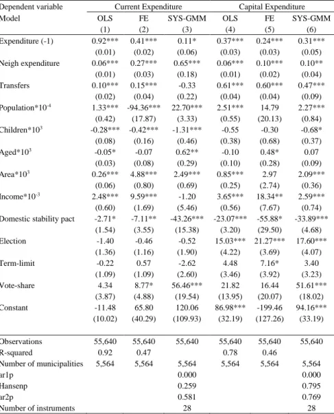
In Table 3 I report the results of the estimations using as dependent variable the two components of total expenditures: current expenditure (col. 1, 2 and 3) and capital expenditure (col. 4, 5 and 6). I apply OLS, FE and SYS-GMM estimators. In the latter case, as before, I instrument the lagged dependent variable and the other endogenous variables (neigh expenditure and transfers) with their lags.

As for the current expenditure, following the estimates of the SYS-GMM, my preferred specification, (Table 3, col. 3), I find a certain degree of persistency in the expenditure, but weakly significant and more modest (0.11) than the one estimated for the total expenditure. The estimated coefficient associated with current expenditure of neighboring muncipalities (neigh expenditure) is positive (0.65), statistically significant at 1% and larger with respect to the one estimated for total expenditure. Such a postive effect suggests that the interaction in current spending decision at the local level is driven by public goods and/or services that are of the complement type.

Moving to capital expenditure, the results - following the estimations of the SYS-GMM (Table 3, col. 6) - show that the estimated coefficient of the lagged dependent variable is positive (0.31), statistically significant at 1%, and very similar to the one estimated for total expenditure (Table 2, col. 3) indicating that capital expenditure at the municipal level in Italy is likely to change slowly over time. The coefficient of capital expenditure of neighboring muncipalities (neigh expenditure) is positive (0.10), signficant at 5%, and lower than the one estimated for total expenditure. The positive coefficient associated to the neighboring expenditure reveals that spatial interactions on capital expenditure at the local level are driven by those investments that are complements in usage. Control variables are also very informative about the determinants of both current and capital municipal expenditure. In particular, the coefficient associated with population*10-4 is positive and significant and thus confirming the presence of congestion effects; the coefficient of per-capita area (area*103_{) is positive and statistically significant, implying}

the presence of economies of scale, and the coefficient of vote-share is positive and significant as I found for the total expenditure. On the contrary, the variable domestic

stability pact, which captures financial constraints imposed by the central government to

municipalities, is negative and significant both for current and capital expenditure. Moreover, for the specific case of current expenditure, the coefficient of aged*103 turns out to be positive and significant, indicating that an higher share of elderly people is associated with higher level of current expenditure. On the side of capital expenditure, instead, the coefficients of transfers (0.47), income*10-3 (2.59) and election (-33.89) play an important role in explaining investment decisions at the municipal level.

Thus far, the empirical evidence leads to three main findings that can be summarized as follows. Firstly, local expenditure of Italian municipalities turn out to be persistent - especially for the case of capital expenditure - and such a result is in line with the evidence found in other countries, such as France (Foucault et al., 2008) and Portugal (Veiga and Veiga, 2007; Costa et al., 2015). Moreover, the results show the presence of a positive horizontal interdependence in spending decision among Italian municipalities, with the effect being more pronounced for current expenditure: a one-euro increase in the average current expenditure of the neighbors generates, ceteris paribus, an increase of 0.65 euro

18

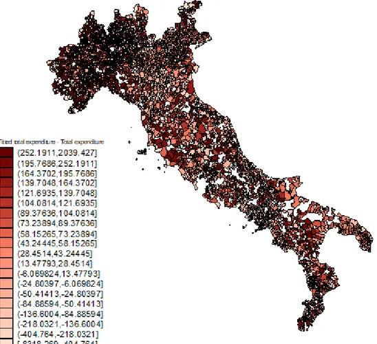
in the municipality’s current expenditure; whereas, a one-euro increase in the average capital expenditures of the neighbors generates, ceteris paribus, an increase of 0.10 euro in municipality’s capital expenditure. While the presence of horizontal interactions in current spending decisions is a well known result for Italian municipalities (Ermini and Santolini, 2011; Bartolini and Santolini, 2012), the findings of a positve interaction in capital expenditure – and thus of a complementarity relationship in the provision of local public goods - represents a novel result for the Italian case. Finally, political variables are important factors of municipal expenditure. In particular, the power of the mayor, in terms of political consensus, leads to higher expenditure – both current and capital – while being in an electoral year positively impacts only on capital expenditure, as spending on infrastructures is usually seen as the most visible expenditure (Drazen and Eslava, 2010). I present the results obtained in the analysis through a colored map in order to show how the spatial effect is distributed across Italian municipalities. Looking at the Figure 1, I notice that the spatial effect is higher in the Northern-east Italy, where there is a high concentration of small municipality in term of land area. This intuition, coming from the map, has been detected in the following analysis, described in the section 1.7.2: the relationship between the spatial effect and the municipality’s dimension.

19

Table 3: Estimation results for current and capital expenditures with the SYS-GMM estimator

Dependent variable Current Expenditure Capital Expenditure

Model OLS FE SYS-GMM OLS FE SYS-GMM

(1) (2) (3) (4) (5) (6) Expenditure (-1) 0.92*** 0.41*** 0.11* 0.37*** 0.24*** 0.31*** (0.01) (0.02) (0.06) (0.03) (0.03) (0.05) Neigh expenditure 0.06*** 0.27*** 0.65*** 0.06*** 0.10*** 0.10** (0.01) (0.03) (0.18) (0.01) (0.02) (0.04) Transfers 0.10*** 0.15*** -0.33 0.61*** 0.60*** 0.47*** (0.02) (0.04) (0.22) (0.04) (0.04) (0.09) Population*10-4 _{1.33*** -94.36*** 22.70*** 2.51*** 14.79 2.27***} (0.42) (17.87) (3.33) (0.55) (20.13) (0.84) Children*103 _{-0.28*** -0.42*** -1.31*** -0.55 -0.30 -0.68*} (0.08) (0.16) (0.46) (0.38) (0.68) (0.37) Aged*103 _{-0.05* -0.07 0.62** -0.10 0.48* 0.07} (0.03) (0.08) (0.29) (0.10) (0.28) (0.09) Area*103 _{0.26*** 4.88*** 2.49*** 0.85*** 2.97 2.09***} (0.06) (0.80) (0.69) (0.25) (2.74) (0.36) Income*10-3 _{2.48*** 9.59*** -1.20 3.65*** 18.34** 2.59***} (0.60) (1.69) (5.46) (0.56) (7.67) (0.74)

Domestic stability pact -2.71* -7.11** -43.26*** -23.07*** -55.88* -33.89***

(1.54) (3.55) (15.38) (3.20) (29.50) (4.68) Election -1.40 -0.46 -0.52 15.03*** 21.27*** 17.60*** (1.36) (1.16) (1.90) (4.22) (3.69) (4.07) Term-limit -0.22 0.57 -2.62 4.48 7.16* 3.40 (1.09) (1.09) (2.60) (3.46) (3.92) (3.23) Vote-share 4.34 8.77* 56.46*** 21.82 16.44 51.61*** (3.87) (4.88) (19.54) (13.95) (20.07) (18.02) Constant -11.48 65.80 120.06 86.98*** -199.46 94.16*** (10.02) (40.29) (109.93) (32.19) (127.26) (33.19) Observations 55,640 55,640 55,640 55,640 55,640 55,640 R-squared 0.92 0.47 0.78 0.46 Number of municipalities 5,564 5,564 5,564 5,564 5,564 5,564 ar1p 0.000 0.000 Hansenp 0.259 0.795 ar2p 0.581 0.769 Number of instruments 28 28

Notes: *** p < 0.01, ** p < 0.05, * p < 0.1. Robust standard errors, clustered at the municipal level, are

shown in parentheses. In all regressions I control for time fixed effects, while, in col. (2), (3), (5) and (6) I also include municipal fixed effects. In col. (3) the variable Expenditure (-1) is instrumented applying difference GMM, by using lags 1, 2, 3 and 4; the variable neigh expenditure is instrumented applying GMM by using lags 7 and 8; the variable transfers (current transfers) is instrumented applying SYS-GMM by using lag 4. In col. (6) the variable Expenditure (-1) is instrumented applying difference SYS-GMM by using lags 1 and 2; the variable neigh expenditure is instrumented applying SYS-GMM by using lags 2 and 3; the variable transfers (capital transfers) is instrumented applying SYS-GMM by using lags 3 and 4. The validity of the instruments is checked by using the standard Hansen test and the C tests (results are available upon request).

20

Figure 1: Maps of spatial interaction effect through Italian municipalities

Notes: the effect is calculated as a mean for the period 2001-2011 by municipality, and as difference between the value of the expenditure of municipality i and the fitted value of the expenditure deriving from the regression of table 2, col. 3 (the stata command used for estimating fitted values is predict x, xb).

21

1.6 Robustness tests

In order to cofirm the results found in the previous Section, I run two set of robustness test. Firstly, I replicated regressions by using alternatve wighting matrices. Then, I employ a quasi-natural experiment, which consists of comparing regression results obtained by relying on an external instrument to the results obtained by using an internal instrument.

1.6.1 Different weighting matrices

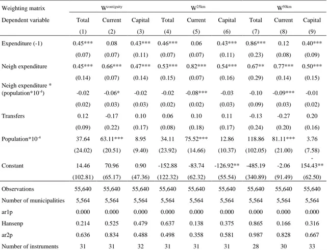
As a first set of robustness test, I re-estimate the previous models by using different neighbor’s matrices. In particular, I define this new neighbors’ variable (neigh

expenditure) by using three weighted matrices. We, first, consider neighbors all

municipalities distant up to 25 km from a given municipality and I weigh the corresponding expenditure with the inverse of that distance; above 25 km the weight is 0. Then, by using the same procedure, I classify as neighbors all municipalities whose distance from a given municipality is no more than 50 km and, finally, I use a broader defintion of neighbors, namely I define neighbors all municiplaities whose distance is within 100 km.

I perform the estimations for the total expenditure and its two components (current expenditure and capital expenditure) using the three spatial matrices, separately. The estimates obtained using a neighbor’s distance less than 25 km confirm the results I have obtained in the previous analysis. The strategic interaction between expenditures persists for each type of expenditure. The coefficient of neighboring expenditure (neigh

expenditure) is 0.22 and significant at 10% when using total expenditure (Table 4, col. 1),

and it is very similar (0.20) for capital expenditure (Table 4, col. 3); however it becomes larger and increases up to 0.77 with current expenditure (Table 4, col. 2).

When I use a neighbor’s distance up to 50 km, the estimates confirm again my previous results for all types of expenditure In particular, when I use total expenditure (Table 4.col. 4) the coefficient of neighbor’s expenditure (neigh expenditure) is 0.34 and statistically significant at 1%. In the other two cases, the neighboring expenditure coefficient takes on the value of 0.88 (at 1% significance) for current expenditure (Table 4, col. 5) and of 0.21 for capital expenditure (Table 4, col. 6).

Finally, when I allow for a wider defintion of neighborhood (100km) the spillover effect vanishes, in fact the coefficient of neighbors expenditure is not stastically significant for total expenditure (Table 4, col. 7), neither for current expenditure (Table 4, col. 8), nor for capital expenditure (Table 4, col. 9).

It is worth noting that although the estimated coefficients are found to be larger as the distance increases16_{, they are not stastically different between each others, leading us to}

16 _{Similar results are found by Costa et al. (2015), who justify the increase in the size of the estimated coefficient by saying that “when}

22

conclude that the spillover effects is not statistically sensitive to the definition of “neighborhood”. In fact, for each of the weighting matrix adopted (25, 50 and 100 km neighborhood) and for the dependent variables (total, current and capital expenditure), I plot the estimated coefficients of the variable neigh expenditure as of Table 4, and its confidence interval at the 10% significance level (Figure A1, Appendix).

As it regards current expenditure, I find that the neigh expenditure coefficient (0.77, and statistically significant at 1%) obtained by using the definition of 25 km neighborhood (Table 4, col. 2) is not statistically different from the coefficient of neigh expenditure (0.88, and statistically significant at 1%) obtained by using the definition of 50 km neighborhood (Table 4, col. 5) since their confidence intervals overlap, while, on the contrary, there is not overlapping between these two coefficients and the estimation of the coefficient of neigh expenditure obtained by using the definition of 100 km neighborhood (Table 4, col. 8), which - as discussed above - turns out to be not statistically different from zero (Figure A1, Panel B, Appendix).

The same picture emerges from both total expenditure (Figure A1, Panel A, Appendix) and capital expenditure (Figure A1, Panel C, Appendix). In particular, for the case of total expenditure, I find that the neigh expenditure coefficient (0.22, and statistically significant at 10%) obtained by using the definition of 25 km neighborhood (Table 4, col. 1) is not statistically different from the coefficient of neigh expenditure (0.34, and statistically significant at 1%) obtained by using the definition of 50 km neighborhood (Table 4, col. 4) since their confidence intervals overlap, while, on the contrary, there is not overlapping between these two coefficients and the estimation of the coefficient of neigh expenditure obtained by using the definition of 100 km neighborhood (Table 4, col. 1), which - as discussed above - turns out to be not statistically different from zero (Figure A1, Panel A, Appendix). Finally, for the case of capital expenditure, the neigh expenditure coefficient (0.20, and statistically significant at 10%) obtained by using the definition of 25 km neighborhood (Table 4, col. 3) is not statistically different from the coefficient of neigh

expenditure (0.21, and statistically significant at 5%) obtained by using the definition of

50 km neighborhood (Table 4, col. 6) as their confidence intervals overlap, while, on the contrary, there is not overlapping between these two coefficients and the estimation of the coefficient of neigh expenditure obtained by using the definition of 100 km neighborhood

investigated further whether the increase in the size of the coefficient is due to heterogeneity across municipalities. In fact, the spillover effect found in my analysis is an average effect of all Italian municipalities and the increase in the size of the spillover effects observed when the distance increases might be linked to some geographical characteristics of municipalities, being the idea that the definition of neighborhood (and so of the distance) is different between municipalities that are located in plain and municipalities that are located in mountain. To address this point we divided municipalities into two groups: the first one contains only municipalities located in plains (2,969 municipalities, 53% of the sample) and the other one contains municipalities located either in hill or in mountains (2,595 municipalities), and we run for these two sub-samples the previous regressions. Interestingly, we found that spillover effects for municipalities located in plain hold only when we use the contiguity matrix, while, for municipalities located in mountain/hill the spillover effects hold with all the weighted matrices and thus suggesting that the size of the spillover effect varies according to definition of neighborhood (and hence of distance), which, in turn, depends on the geographical characteristics of municipalities. Results are available upon request.