12th Joint European Thermodynamics Conference Brescia, July 1-5, 2013
NON-EQUILIBRIUM TEMPERATURES IN SYSTEMS WITH INTERNAL
VARIABLES
David Jou *, Liliana Restuccia**
* Universitat Aut `onoma de Barcelona, Grup de Fis´ıca Estad´ıstica, 08193 Bellaterra, Catalonia, Spain, E-mail: [email protected]
** University of Messina, Department of Mathematics, Viale F. Stagno D’Alcontres 31, 98166 Messina, Italy, E-mail: [email protected]
ABSTRACT
We discuss different definitions of non-equilibrium temperature in systems with internal variables. In equilibrium states, all the different definitions of temperature (caloric, entropic, kinetic, vibrational, configurational, fluctuational, and so on) lead to the same value, but in non-equilibrium they lead to different values. Out of equilibrium, equipartition is not to be expected and therefore the ”temperatures” of the different degrees of freedom will be different from each other. Here, we focus our attention on the caloric temperature, based on the internal energy corresponding to the internal variable, the entropic temperature, based on the entropy, and several thermometric or empirical temperatures, based on the zeroth law. We illustrate the difference and the connections between them in some simple systems with a heat flux (two-level and three-level systems, ideal gases), and we also consider a solid system with internal variables. These variables may be measured, but not controlled, and they appear in the Gibbs equation like the classical thermodynamic variables. As an example, we consider a crystal with dislocations submitted to an external flux of energy (like a wall of a fusion reactor bombarded by energetic particles).
INTRODUCTION
Temperature is a concept common to all thermodynamic ap-proaches. However, the meaning and measurement of tem-perature in non-equilibrium steady states beyond the local-equilibrium approximation is one of the fundamental problems in advanced non-equilibrium thermodynamics. Thus, it is log-ical that different approaches may consider temperature from different perspectives. For instance, in rational thermodynam-ics, it is considered as a primitive quantity. In theories with internal variables, each variable could have in principle its own temperature. In extended thermodynamics, temperature is as-sumed to depend also on the fluxes. In statistical theories, tem-perature may be related to the form of the distribution functions. Thus, a comparative discussion of the several thermodynamic approaches requires as a preliminary condition to compare and clarify the role of temperature.
Wide surveys of this topic are in [1]-[5]. Out of equilibrium, energy equipartition is not expected and, therefore, different measurements of temperature, sensitive to different sets of de-grees of freedom, will yield different values for the temperature. From the theoretical perspective as well, different definitions of temperature will also lead to different values of this quantity.
For instance, in a system composed of matter and radiation, a thermometer with purely reflecting walls will give the tem-perature of matter, as it will be insensitive to radiation. In contrast, a thermometer with perfectly black walls will yield a temperature related both to matter and radiation. In equilib-rium, both thermometers will give the same temperature, but in a non-equilibrium steady state (for instance, with photons trans-mitting heat and colliding against the particles of a gas) these thermometers will give different temperatures.
Another situation with several -or many-temperatures arises
in mixtures of gases with internal degrees of freedom and at high temperatures, as in the entry of spaceships into a plane-tary atmosphere. In such a case, one may have different kinetic temperatures for different gases, and different electronic tem-peratures (related to the relative occupancy of electrons at the several energy levels), and different vibrational and rotational temperatures. All these temperatures may be experimentally obtained by means of spectrometric methods, by measuring the intensity of the spectral lines emitted by the gases.
As it was pointed out in [1], instead of trying to attribute to some of the mentioned temperatures a more relevant role than to others (this will be indeed the case, but for different kinds of temperatures depending on the problem being addressed to), one should try to obtain the relations between them when the conditions on the system (total energy, energy flux, and so on) are specified. In fact, the ensemble of these different temper-atures yields a very rich information about the system: about their internal energy transfers and their internal energy contents for the several degrees of freedom.
Here, we will discuss in detail the thermometric, caloric and entropic temperatures for systems with internal variables, the first one related to the zeroth law, the second one being based on the internal energy of the variable, and the third one related to its entropy.
TEMPERATURE DEFINITIONS IN EQUILIBRIUM THERMODYNAMICS
In equilibrium thermodynamics there are several definitions of temperature: empirical (based on the zeroth law), caloric (based on the first law), and entropic (based on the second law). Here, we remind the reader these definitions.
Empirical (or thermometric) temperature is defined by the ze-roth law, which states the transitive character of thermal equi-librium. In particular, it states that if a state A of a system is in equilibrium with state B of another system, and state B is in equilibrium with state C of a third system, states A and C are in mutual thermal equilibrium.
Entropic definition:
The most fundamental definition of temperature in equilibrium thermodynamics is that appearing in the Gibbs equation.
1 T¥˙ µ ∂S ∂U ∂
all other extensive variables
, (1)
where the subscript ”all other extensive variables” means that the derivative must be carried out keeping constant all the other extensive variables appearing in the entropy, as for instance the volume V , the number of particles Niof the species i and so on.
Caloric definition:
Another definition of temperature - we will call it the caloric definition, because it uses the so-called caloric equation of state relating internal energy and temperature - is obtained from the internal energy of the different degrees of freedom. For instance
U = U(T,V, Ni). (2)
Since U is defined by the first principle, this definition is related to this principle.
TEMPERATURE DEFINITIONS IN STEADY STATE NON-EQUILIBRIUM THERMODYNAMICS
Our aim is to explore in a few simple situations how the tem-peratures defined by (1) and (2) differ in non-equilibrium steady states. Non-equilibrium steady states are different than equilib-rium states because in them the system is crossed by fluxes of energy, matter, electric current and so on. Thus, it is interesting to investigate the influence of such fluxes on the thermodynam-ics of the system. The presence of fluxes is related to inhomo-geneities in the system: the presence of a gradient of tempera-ture, concentration, electrical potential or barycentric velocity.
Illustration 1: caloric and entropic temperatures in two-level system with an energy flux
First, we present an example related to a statistical descrip-tion [6]. We illustrate the mendescrip-tioned concepts of temperature with a two-level system, with N1particles at level 1 (with energy
E1) and N2particles at level 2 (with energy 2). For instance, this
could refer to electrons in two electronic levels, or to spins un-der an external magnetic field, or some other situations. The total internal energy will be U = N1E1+ N2E2; from here, one
may define a caloric temperature T as
kBT¥N1
N E1+ N2
NE2, (3)
with N the total number of particles N = N1+ N2, and kB the
Boltzmann constant. On the other side, in equilibrium situations following the canonical distribution function, the temperature
will be defined as
kBT ¥ E2° E1
ln(N1/N2). (4)
Assume now that the system is submitted to an energy flow q (energy per unit time), in such a way that the relative proportion of particles in states 1 and 2 is modified (for instance, the higher energy level 2 becomes more populated than in equilibrium, and the lowest level, which is receiving the external energy, becomes less populated).
Assume that the dynamics of the populations N1 and N2is
given by
dN1
dt = ° dN2
dt = °αN1+ βN2° γqN1, (5) where α and β are the transition rates from 1 to 2 and from 2 to 1 respectively, and γ is a coefficient related to efficiency of energy absorption by particles in the lower level 1 bringing them to the higher level 2. The steady state solution of (5) is
N1
N2 =
β
α + γq. (6)
For q = 0, one has N1 N2 =β α= exp ∑ °E1k° E2 BT ∏ . (7)
This is the detailed-balance relation amongst the rates. By keeping the definitions (3) and (4) but related to the non-equilibrium populations, one gets the following expressions for the non-equilibrium caloric temperature
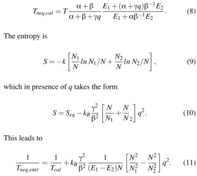
Tneq,cal= T α + β α + β + γq E1+ (α + γq)β°1E2 E1+ αβ°1E2 . (8) The entropy is S =°k ∑ N1 Nln N1/N + N2 N ln N2/N ∏ , (9)
which in presence of q takes the form
S = Seq° kBγ 2 β2 ∑N N1 +N N2 ∏ q2. (10) This leads to 1 Tneq,entr = 1 Tcal+ kB γ2 β2 1 (E1° E2)N ∑ N2 N2 1 °N 2 N2 2 ∏ q2. (11)
Finally, the non-equilibrium thermometric temperature from (4) and (6) will be Tneq,th= T 1 1°ln[1+(γ/α)q]E 2°E1 kBT . (12)
It is seen that these temperatures are different from each other when q6= 0. Here, T is the equilibrium temperature, which is equal to the temperature of a thermal bath in which these sys-tems are in contact. Note that in the extreme situations that the higher-level population 2 becomes higher than the lower level population 1, namely, for q higher than (β° α)/γ , the entropic temperature becomes negative, whereas the caloric temperature remains positive. Note that a thermometer in equilibrium in contact with the system will measure temperature (12), rather than temperature (8) or (11). From temperature (12) it would be possible measure γ. Spectrometric methods allow to measure temperature (12) through the intensity of spectral emission line corresponding to 2! 1.
Illustration 2: thermometric temperature in three-level sys-tem with an energy flux
To discuss the problems related to zeroth law and thermo-metric temperature we consider a three-level system, with ener-gies E1< E2< E3, and assume, for the sake of simplicity, the
simplest triangular scheme for its possible internal transitions, namely 1! 2 ! 3 ! 1. More realistic schemes are possible, but here we want to stick to the simplest illustrations. The evo-lution of the atomic populations N1, N2and N3will be given by
dN1 dt = °α1N1+ βN3° γ1qN1, dN2 dt = °α2N2° γ2qN2+ α1N1+ γ1qN1, dN3 dt = ° dN1 dt ° dN2 dt , (13)
where α1, α2and β stand for the rate transitions coefficients; in
particular, γ1and γ2stand for the part of the energy flux which
interacts with particles in state 1 and in state 2. The steady state populations will be N1 N2 =α2+ γ2q α1+ γ1q, N1 N3 = β α1+ γ1q . (14)
The equilibrium temperature will be
kBT =
E2° E1
ln(N1/N2)
= E3° E1
ln(N1/N3). (15)
The thermometric temperatures related to populations 1 and 2, as 1 and 3 , will be the following non-equilibrium temperatures
Tneq,12= T 1 1°ln[(1+(γ1/α1)q)/(1+(γ2/α2)q)] E2°E1 , Tneq,13= T 1 1°ln[1+(γ1/β1)q] E3°E1 . (16)
A thermometer in contact with levels 1 and 2 would measure T12, and a thermometer in contact with 1 and 3 would measure
T13; analogously, a thermometer in contact with 2 and 3 would
measure a temperature T23 defined in analogy with (16)a and
(16)b. Of course, in equilibrium all these temperatures would
be the same. It is not clear, instead, what would measure a ther-mometer in contact with 1, 2 and 3. From expressions (16) it would be possible to obtain γ1and γ2. Note, therefore, that the
zeroth-principle of equilibrium thermodynamics cannot be ap-plied to non-equilibrium steady states.
Illustration 3: caloric and entropic temperatures in non-equilibrium ideal gas
Ideal gases are a system for conceptual discussion of thermo-dynamic concepts [7], [8]. In kinetic theory, the temperature of a gas is usually defined as the kinetic temperature, which is a form of caloric temperature, through the relation
3
2kBT =< 1 2mC
2>, (17)
where m and C are the mass and the velocity intensity of a gas particle, respectively. This relation has nothing to do with the special form of the distribution function. In non-equilibrium states, the distribution function may be written as
f (r,C,t) = feq(r,C,t)[1 + Φ], (18)
with feq the equilibrium distribution function characterized by
the local values of the thermodynamic parameters, and Φ a non-equilibrium contribution. Up to the second order in Φ , the ”en-tropy” s obtained from the H-function has the form
s = seq°1
2kB
Z
feqΦ2dC, (19)
with s the entropy per unit volume. It is seen that, in principle, s will be different from the local-equilibrium entropy seq. Then
one may define the entropic temperature as 1 Tneq,ent =∂s ∂u= 1 T ° kB 2c ∂ ∂T Z feqΦ2dC. (20)
In a system submitted to a heat flux, the entropy (19) has the form, up to the second order in the heat flux,
s = seq° τ
2λT2q· q, (21)
where τ is the collision time and λ the thermal conductivity. In more explicit terms, taking into account that
λ =5 2kB
p
the general expression (21) combined with definition (20) yields 1 Tneq,ent = 1 T + 2 5 nm p3Tq· q. (23)
This temperature would be merely formal unless a method of measurement of it may be specified. It has been shown that this non-equilibrium temperature corresponds to the kinetic temper-ature in the plane perpendicular to the heat flux. Thus, if the heat flux is in the z direction, one has
<1 2mC 2 x>=< 1 2mC 2 y>= 1 2kBTneq,ent< 1 2kBT and <1 2mC 2 x>= 1 2kB(3Tneq,ent° 2T ) > 1 2kBT (24) in such a way that the usual definition of T given in (18) is satis-fied. Thus, the concept of the entropic definition of temperature is not in contradiction with that of the kinetic definition.
NON-EQUILIBRIUM TEMPERATURES IN CONTIN-UUM THERMODYNAMICS
Here, we formulate the problem in the framework of contin-uum thermodynamics and we consider non-equilibrium steady states, different than equilibrium states because in them the sys-tem is crossed by fluxes of energy, matter, electric current or so on. In classical irreversible thermodynamics it is assumed the local equilibrium hypothesis, that states that the fluxes have not an essential influence on the thermodynamics of the system. It assumes that a continuous system out of equilibrium may be decomposed in many small subsystems, each of which behaves, from a thermodynamic point of view, as if it was in local equi-librium.
Non-equilibrium steady states are the natural generalization of equilibrium states: in them, the values of the variables do not depend on time but, in contrast to equilibrium states, a continuous flux of energy or matter, or momentum, or charge -must be supplied and extracted from the system. We recall the well-known Fourier’s transport equation for heat flow q
q =°λ∇T, (25)
with λ the thermal conductivity.
Beyond local equilibrium, for an ideal monoatomic gas, the entropy takes the form (21), which writes as
s(u, q) = seq(u) ° α(u)q · q, (26)
where s and u are the entropy and the internal energy, respec-tively, per unit volume and α =° τ(2λT2)°1. Using definition
(1) we have for the entropic temperature θ 1 θ= µ ∂s ∂u ∂ q = 1 T ° µ ∂α(u) ∂u ∂ q· q, (27)
with T the caloric temperature. In a steady state we can use
q =°λ∇T and rewrite relation (27) in the form
s(u, q) = seq(u) ° τλ
2T2∇T· ∇T. (28)
Non-equilibrium temperatures in solid systems with inter-nal variables
In this section we will discuss the caloric and entropic non-equilibrium temperatures in a crystal with dislocations, submit-ted to a given energy flux. We have in mind, for instance, the walls of a fusion nuclear reactor, which are submitted to an in-tense neutron flux supplied by the nuclear reaction or an elec-tronic device with hot electrons. The neutron flux has two ef-fects on the walls: a thermal effect (it heats them), and a me-chanical effect (it produces dislocations in the walls). The sec-ond effect is unwanted, because it may reduce the mechanical resistance of the wall.
We assume that in the considered medium we have fol-lowing fields [9]-[11]: the elastic field described by the to-tal stress tensor ti j and the small-strain tensor εi j, defined by
εi j=12(ui, j+uj,i) (being uithe components of the displacement
vector), the thermal field described by the local temperature θ, and the heat flux qi. However, we assume that the description of
the evolution of the system requires the introduction of further dynamical variables in the thermodynamic state space like, for instance, an internal variable. But, whereas the classical vari-ables may be measured and controlled, the internal varivari-ables cannot be controlled. In solid media they can describe internal defects like dislocation lines, point defects, porous channels, disclinations and so on. They appear in the Gibbs equation like the classical thermodynamical variables. The evolution of inter-nal variables is described by rate equations, different from the constitutive relations, the transport equation of heat, the balance equations of mass, momentum, momentum of momentum and energy. The whole set of these equations describe the evolution of the system.
Thus, we introduce in the thermodynamic state space the in-ternal variable ai jand its flux Vi jk.
We assume that the evolution equation for the tensorial inter-nal variable is the following
dai j
dt +Vi jk,k= Ai j, (29) where ai jis the dislocation core tensor, Vi jkis its flux and Ai jis
a field source. The tensor ai j, introduced by Maruszewski [12],
describes the local structure of dislocations lines, which form a network of very thin lines disturbing the otherwise perfect peri-odicity of the crystal lattice. Since these very thin channels, in general, are not distributed isotropically, it is natural to describe them by a tensor, taking into account the local density of the dislocation channels along several directions
The tensor Ai jrepresents the source-like term describing the
net effects of formation and annihilation of dislocation lines, which may be a function of temperature T , the strain tensor εi j,
the energy flux q, or the stress tensor ti j. Equation (29) could
be simplified, for instance, by assuming for the dislocation flux Vi jk= °D∂a∂xi jk, with D being a diffusion coefficient for
combination of a formation term and a dislocation-destruction term, namely, Ai j= Ai j(formation)°Ai j
(destruc-tion).
Then, we consider for the evolution equation for the internal variables the simple form
dai j
dt ° D∇
2a
i j= Ai j,eq+ ˜αqiqj. (30)
Here, Ai j,eqis the net formation tensor in the absence of an
ex-ternal energy flux (q = 0), and we have added to it a tensor depending on the energy flux.
This form does not pretend to be especially realistic, but only to illustrate that thermal stresses related to qiqjcould influence
the evolution of dislocation lines. More realistic than a simple energy flux, would be to consider, for instance, an energy flux due to the bombardment of the crystal with particles having rel-atively high energy, which could produce new defects or modify the structure of the dislocation lines.
Non-equilibrium entropic temperature
The entropic definition of absolute temperature is related to the Gibbs equation which, for the system we are considering, has the form
ds = θ°1dU + θ°1σi jdεi j° θ°1πi jdai j° θ°1πdqi, (31)
with πi jthe corresponding thermodynamic potential conjugate
of the dislocation tensor ai j and π the corresponding
thermo-dynamic potential conjugate of the heat flux qi. Here, u is the
total internal energy of all the degrees of freedom, and we call θ the entropic (absolute) temperature to distinguish it from the T related to the caloric definition.
We have assumed that only the internal variable under con-sideration is modified by the presence of an external energy flow. Of course the classical variables, like U and εi jwill also
be modified by the flux, but here we refer to the modification of temperature for given values of the classical variables.
The thermodynamic absolute temperature is given by (1). In particular, for given values of the classical variable εi j and
in steady states, the equilibrium temperature and the non-equilibrium temperature are defined by
θ°1eq ¥˙ µ ∂s ∂u ∂ q=0 ; θ°1neq¥˙ µ ∂s ∂u ∂ q6=0 . (32)
The quantity θ°1neq can be expanded around its equilibrium
counterpart obtaining
θ°1neq= θ°1eq ° θ°2eq
∂θeq
∂ai jΔai j, (33)
where in steady states
Δai j= ai j(q 6= 0) ° ai j(q = 0). (34)
Then, in the first approximation, the non-equilibrium tempe-rature θneqwill be related to the equilibrium temperature
corre-sponding to ai j(q = 0) as θneq= θeq 1° θ°1eq ∂θ∂aeqi jΔai j º T µ 1 + T°1 µ ∂T ∂ai j ∂ Δai j ∂ = T + µ ∂T ∂ai j ∂ Δai j, (35)
where we have taken into account that in equilibrium (or local-equilibrium) all the definitions of temperature coincide, there-fore θeq= T , and we have used the approximation (1 ° x)°1º
1 + x, for xø 1.
Non-equilibrium caloric temperature
To define the caloric definition of temperature first we con-sider the caloric equation of state at the equilibrium of the sys-tem for given values of εkland for vanishing values of the
exter-nal flux q: Udis= U (ai j(T,εkl),T,εkl), where we have taken in
consideration that at equilibrium the internal variable depends on temperature and the stress tensor. Then, we define the caloric non-equilibrium temperature field Tneqrelated to ai jin a steady
state in the following way
Udis(ai j(Tneq, εkl, q = 0), Tneq, εkl) ˙¥ Udis(ai j(T,εkl, q), T, εkl)).
(36) Then, to define the caloric non-equilibrium temperature as-sume that the formal expression of the relation between inter-nal energy and temperature keeps, out of equilibrium, the same form as in equilibrium ( Udis = U (ai j(T,εkl),T,εkl) ), where
q = 0, and we equate it to the value of internal energy in
non-equilibrium, where q6= 0. Thus, we define the tempera-ture in non-equilibrium state as that temperatempera-ture which, intro-duced in the caloric state equation would give for the internal energy the actual value corresponding to the non-equilibrium state. Namely, we will have
Tneq= T + µ ∂T ∂Udis ∂ ΔUdis= T + µ 1 cdis ∂ ΔUdis, (37) where≥∂U∂T dis ¥
ΔUdisis the non-equilibrium contribution due to
the presence of q6= 0, and cdisis the specific heat associated to
the changes of the internal energy of dislocation lines, per unit volume, namely cvdis =∂U∂Tdis. The specific heat plays thus an
important role in the caloric definition of temperature.
Entropic flux in the definition of non-equilibrium tempera-ture
In [1] it was seen that in the case of a crystal with disloca-tions, the entropy flux has the form
JkS= θ°1qk° πi jθ°1Vi jk. (38)
Here, the variable πi j is the conjugate to ai j as introduced in
(31). It has been proposed that a convenient definition of a non-equilibrium contribution could be based on this expression (38),
taking as the reciprocal of thermodynamic temperature the co-efficient linking the heat flux q with the entropy flux JS. Based on the idea of perfect interfaces between systems, in which both the heat flux and the entropy flux would be continuous, Muller gave the definition of the so-called ”coldness”, namely, of the reciprocal of absolute temperature.
Considering the entropy flux and the heat flux through an in-terface between two systems (let us say, a thermometer and a system) is convenient, because this reminds us the importance of the contact between the system and the thermometer in mea-suring temperature.
In this aspect, problematic questions arise. In first place, the existence of ideal interfaces is a nice theoretical concept, but in general the interfaces between different materials are not ideal, but exhibit the so-called ”thermal boundary resistance”, which implies a discontinuity of temperature through the surface, and a corresponding discontinuity of the entropy flux, due to entropy production across the wall, due to the fact that heat is flowing between two different temperatures.
FINAL COMMENTS
In this presentation we have emphasized that one of the aims of non-equilibrium thermodynamics should be to find the trans-formation laws relating several thermometric, entropic, caloric and other temperatures in systems submitted to given energy flux.
This program has been partially carried out in [1] for forced harmonic oscillators in a thermal bath, in which case kinetic and vibrational temperatures play a special role, and for ideal gases in Couette flow [13], for kinetic temperatures along the three spatial axes, thermodynamic absolute temperature, local-equilibrium temperature, and fluctuation dissipation tempera-ture, or the relation among some non-equilibrium temperatures in heat transport along nanowires [14].
Here, we have tried to be more general, both by the use of simple illustrations of two-level, three-level systems and ideal gases, as by the statement of this problem in the context of a more difficult and demanding situation of solids systems with dislocations.
REFERENCES
[1] J. Casas-Vazquez and D. Jou, Rep. Prog. Phys. 66bb , p. 1937, 2003.
[2] J. G. Powles, S. G. Rickayzen and D. M. Heyes, Temper-atures: Old, New and Middle Aged, Mol. Phys., vol. 103, pp.1361-1373, 2005.
[3] W. G. Hoover and C. G. Hoover, Non-Equilibrium Tem-perature and Thermometry in Heat-Conducting Models, Phys. Rev. E, vol. 77, 041104, 2008.
[4] E. Bertin, K. Martens, O. Dauchot and M. Droz, Intensive Thermodynamic Parameters in Non-Equilibrium Systems, Phys. Rev. E, vol. 75, 031120, 2007.
[5] R. S. Johal, Quantum Heat Engines and Non-Equilibrium Temperature, Phys. Rev. E, vol. 80, 041119, 2009. [6] L. E. Reichl, A Modern Course in Statistical Physics,
Uni-versity Texas Press, Austin, 1998.
[7] D. Jou, J. Casas-Vazquez and G. Lebon, Extended Irre-versible Thermodynamics, Springer, Berlin, fourth edition, 2010.
[8] D. Jou and L. Restuccia, Mesoscopic Transport
Equa-tions and Contemporary Thermodynamics: an Introduc-tion, Contemporary Physics, vol. 52, 5, pp. 465-474, 2011. [9] W. Muschik, Non-Equilibrium Thermodynamics with Ap-plications to Solids, Springer, Wien-New York, vol. 336, 1993.
[10] L. Restuccia, Thermomechanics of Porous Solids Filled by Fluid Flow, in E. De Bernardis, R. Spigler and V. Va-lente (ed.) , Series on Advances in Mathematics for Ap-plied Sciences, ApAp-plied and Industrial Mathematics in Italy III, vol. 82, pp. 485-495, World Scientific, Singapore, 2010.
[11] L. Restuccia, On a Non-conventional Thermodynamical Model of a Crystal with Defects of Dislocation, to be pub-lished.
[12] B. T. Maruszewski, On a Dislocation Core Tensor, Phys. Stat. Sol.(b), vol. 168, p.59, 1991.
[13] M. Criado-Sancho, D. Jou and J. Casas-Vazquez, Non-equilibrium Kinetic Temperature in Flowing Gases, Phys. Lett. A, vol.350, pp. 339-341, 2006.
[14] D. Jou, V. A. Cimmelli and A. Sellitto, Non-Equilibrium Temperatures and Second-Sound Propagation along Nanowires and Thin Wires, Phys. Lett. A, vol. 373, pp. 4386-4392, 2009.