Contents lists available atScienceDirect
Computers and Mathematics with Applications
journal homepage:www.elsevier.com/locate/camwaAdaptive grid modelling for cancer cells in the early stage
of invasion
Antonino Amoddeo
∗Department of Civil, Energy, Environmental and Materials Engineering, Università ‘Mediterranea’ di Reggio Calabria, Via Graziella 1, Feo di Vito, I-89122 Reggio Calabria, Italy
a r t i c l e i n f o
Article history:
Received 16 October 2013
Received in revised form 3 November 2014 Accepted 15 January 2015
Available online 26 February 2015
Keywords: FEM MMPDE Cancer invasion Avascular growth uPA system
a b s t r a c t
Modelling the interaction of the urokinase plasminogen activator system with a model for cancer cells dynamics lead to a system of five coupled partial differential equations the solution of which, over a one-dimensional domain, can be obtained using the finite element method. As the discretization of the integration domain is crucial, particularly in the presence of strong variations of the domain variables, we tackle the problem solution implementing an adaptive grid numerical technique. Our results improve previous numerical simulations performed on uniformly discretized domains, allowing to capture finer spatial details characterizing the interface between cancer and healthy cells, which can be related to malignancy: low values of the cancer cells motility induce a high spatial heterogeneity at the cancer/healthy cells interface, while the dynamical evolution over the whole domain shows branched spatio-temporal patterns; on the contrary, higher motility values smooth the cancer cells spatial profile, letting cancer cell concentration to evolve according to a less heterogeneous pattern.
© 2015 Elsevier Ltd. All rights reserved.
1. Introduction
The dynamical evolution of cancer cells is a mechanism strongly interconnected with phenomena occurring over different length scales: at microscopic level, sub-cellular mechanisms such as DNA degradation, gene expression, nutrient absorption, etc., influence intercellular interactions in both tumour and healthy cells; such mesoscopic phenomena determine the evolution at the tissue level, thus the need for multiscale approaches accounting for complexes modelling arises [1–3], a field which is fast developing together with the increasing in computational power. Schematically, at tissue level cancer cells start to cluster in the avascular phase, building multicellular spheroids [4–8] and are possibly attacked by the immune system; after the mechanical interaction with the surrounding tissue [9–11], tumour cells stimulate the angiogenesis process causing the formation of new blood vessels and attracting nutrients [12–16]; at this stage the tumour enters the vascular phase attracting much more nutrients like oxygen and glucose [17–19]: the increased speed of invasion of the healthy cells and the vascularization allow cancer cells to break-out from the initial localization, beginning metastasis through the vascular system [15,20–22], giving them their deadly characteristic. Recent reviews focusing on mathematical modelling of cancer cell growth and proliferation can be found, among others, in Refs. [23–29].
Avascular tumour growth models can be grouped within three categories: continuum models expressed as systems of Partial Differential Equations (PDEs), discrete approaches, and hybrid continuum/discrete combinations [30]. At tissue level,
∗Tel.: +39 0965 875299; fax: +39 0965 875201.
E-mail address:[email protected]. http://dx.doi.org/10.1016/j.camwa.2015.01.017 0898-1221/©2015 Elsevier Ltd. All rights reserved.
the continuum approach is appropriate, and the tumour is modelled as a cluster of cells immersed in the extracellular matrix (ECM), an aqueous environment containing nutrients, like proteins, oxygen, and glucose; here, depending on chemical signalling, cancer cells start to grow and proliferate [1]. Models based on the assumption that the cancer cells movement is in response to chemotactic and/or haptotactic stimuli have been recently developed [31], as the coupling of the urokinase plasminogen activator (uPA) system to a model of cancer cells invasion [32,33]. In this respect, these latter papers focus on the role of the uPA system in the ECM degradation, which is a key process in tumour invasion of a healthy tissue: in such process, the proteolysis of the ECM macromolecules is catalyzed by a degrading enzyme, specifically the uPA serine protease [34,35]. Broadly speaking, the invasion starts from the degradation of the ECM components such as the vitronectin (VN) protein; to do so, cancer cells secrete the enzymatically inactive pro-uPA, which is activated to uPA by plasmin, an ECM degrading enzyme, being in turn an activated form of the plasminogen ubiquitous protein, and both uPA and pro-uPA bind to the receptor pro-uPAR, binding, in turn, to the cell surface; on the other hand, the excess of proteolysis induced by uPA is also prevented by the plasminogen activator inhibitor type-1 (PAI-1), a specific inhibitor secreted by healthy cells. For a detailed description of the biological mechanisms involved, see Chaplain and Lolas [32], Andasari et al. [33], in which the uPA system is intended as constituted by the uPA itself, the plasmin, the VN protein, and the PAI-1 inhibitor. These authors couple the cancer cell dynamics to the uPA system obtaining, in a continuum framework, a system of five coupled PDEs solved in both one and two dimensional domains, imposing a set of model parameters, and suitable initial and boundary conditions for times t
∈
(
0,
T]
. In particular, ifΩ1:=
(
0,
M)
, with M a positive scalar parameter, is a onedimensional spatial domain understood as a one dimensional portion of biological tissue, whileΩ2
:=
(
0,
M) × (
0,
M)
, isa two dimensional region of tissue, they performed the integration of the PDE system using a code based on the method of lines, using a uniform finite volumes discretization in space, over theΩ1
×
(
0,
T]
, orΩ2×
(
0,
T]
, integration domains, and animplicit method for discretization in time. The main result of such a model, in which a linear stability analysis is also provided, is the prediction that cancer invasion proceeds through spatio-temporal patterns having a degree of inhomogeneity which depends upon the motility of the cancer cells; while 2D simulations are in qualitative agreement with previous experimental results [36,37].
Nevertheless, just the high irregularity of the spatio-temporal proliferation patterns they obtained, suggests that the overall accuracy of the numerical procedure could be influenced by the discretization of the integration domain: in fact, as the spatial positions at which cancer cell cluster are a priori unknown, the choice of an appropriate grid of points is crucial, particularly in the presence of local steep gradients of the domain variables.
Recently, computer simulations of solid tumour growth have been performed in two and three dimensions implementing adaptive meshing and multi-grid algorithms in order to improve the effectiveness of the computational techniques [38,39], while a hybrid finite volume/finite element algorithm has been used to discretize a continuum model for a vascular tumour growth [30]. The Finite Element Method (FEM) is used for application in several research branches, and provides computational mathematics with a powerful tool to solve PDEs systems arising from problem modelling [40]: the integration domain is discretized in elements composed by nodes on which the solution of a domain variable is found, while its spatial variation inside each element is interpolated by suitable shape functions.
In general, adaptive grid techniques can be either static (h- or p-type) or dynamic (r-type), and allow resolution improvements and computational savings with respect to techniques based on uniform discretizations [41]. h-type remeshing methods rely on the insertion of extra mesh points in order to satisfy tolerance requirements, while p-type techniques keep constant the number of nodes increasing the order of the polynomial used to represent the solution within each element. Unfortunately, static remeshing techniques can lead to an undesired huge amount of points, memory and time consuming (h-type), or can be limited by smoothness requirements (p-type). r-type techniques, also known as moving mesh techniques, instead, keep constant the nodal connectivity and number of mesh points inside the domain: simply, the mesh points are moved towards regions where more details are required, with no need for external intervention.
Facing the modelling of highly frustrated dynamical system, recently we have developed a numerical technique allowing effective and reliable numerical solutions of PDEs system over a one dimensional integration domain where relevant temporal and/or spatial variations of some physical parameters occur [42–45]. Specifically, we have implemented the moving mesh partial differential equations (MMPDEs) numerical technique using FEM to solve a system of six coupled non-linear PDEs arising from the problem modelling of a nematic liquid crystal confined between plates, submitted to strong electrical and mechanical stresses. In such method, the discretization of the integration domain is not uniform, but it is driven by the gradient of a suitable order parameter which is calculated during the solution procedure: the technique concentrates the grid points in regions of large variations of the chosen parameter, maintaining constant the number of the nodes in the domain, thus ensuring no waste of computational effort in areas of low spatial variability where there is no need for finer grids, thus allowing an overall resolution improvement. The model developed in [33] predicts highly inhomogeneous patterns for the cancer cell dynamics, suggesting that the use of an adaptive remeshing technique as a tool to improve the model resolution in regions of the integration domain where steep gradients of the cancer cell concentration are present could be appropriate. Following such idea, this work is concerned with the implementation of the MMPDE technique to the model introduced in Ref. [33], aimed at demonstrating the validity of our technique applied to the one dimensional model there presented: our numerical simulations, in fact, improve the model resolution and give a new insight about the challenging problem of the cancer cell proliferation. The paper has the following organization: in Section2the theoretical model of the uPA system coupled with the cancer cell dynamics is highlighted; the numerical technique is presented in Section3, while the numerical results are discussed in Section4. Finally, we conclude in Section5.
2. Theoretical model
LetΩ
∈
R3be a fixed volume domain and S its bounding surface, the variation of a cell population, having density c(
x,
t)
at time t
∈
(
0,
T]
and position x∈
Ω, is governed by the conservation lawd dt
V c(
x,
t)
dx= −
Sϕ(
x,
t) ·
dS+
V f(
c,
s)
dV (1)where
ϕ(
x,
t)
is the flux of the cells through S; f accounts for cells production and depends also on the vector valued function s representing the concentration of the n interacting chemical species present in the simulated domain: hence,s
=
(
s1, . . . ,
sn)
, in which each sı=
si(
x,
t)
, for i=
1, . . . ,
n. Using the divergence theorem, assuming the domain fixed intime, given the arbitrary volume V , the PDE describing the evolution of the cell population c
(
x,
t)
is obtained∂
c∂
t= −∇ ·
ϕ +
f(
c,
s).
(2)With similar considerations, the evolution equations for the other species sican be obtained
∂
si∂
t= −∇ ·
ψ
i+
γ
i(
c,
s),
i=
1, . . . ,
n (3)where
ψ
iandγ
i, account for, respectively, flux and production terms for the ith species. Eq.(2)and the n Eqs.(3)constitutea system of n
+
1 coupled PDEs to be solved in order to describe the dynamics inside the domainΩ. Following Andasari et al. [33], we denote the cancer cells concentration by c(
x,
t)
, the VN concentration byv(
x,
t)
, the uPA concentration byu
(
x,
t)
, the PAI-1 concentration by p(
x,
t)
, and the plasmin concentration by m(
x,
t)
.Cell movement inside the ECM can be promoted by at least two distinct mechanisms, chemotaxis and haptotaxis, being both directional motility mechanisms in response to concentration gradients of chemicals influencing cell migration: in the first case, cancer cells sense the chemicals dissolved in solution and move eventually reaching their source; the second mechanism rely on the adhesion of the attracting chemicals to some ECM component: cancer cells move by iteratively making and breaking bond with such chemicals, ‘jumping’ towards growing concentration gradient of molecules adhered to ECM. In Eq.(2), the flux vector takes into account the random motility of cancer cells Dc, as well as chemotaxis due to the
presence of uPA and PAI-1 molecules, respectively through
χ
uandχ
p, and haptotaxis due to VN, throughχ
v. In addition,cells proliferation is accounted for with the inclusion of a logistic growth term, through the cancer cell proliferation rate
µ
1.Considering Eq.(3), as we are in presence of four different chemical species, hence n
=
4, it gives the evolution equation of, respectively, VN, uPA, PAI-1 and plasmin. ECM does not diffuse, so we putψ =
0; on the other hand, VN is degraded by plasmin at a rateδ
and neutralized by PAI-1 inhibitor at a rateφ
22, while the PAI-1-uPA interaction indirectly supports VNgrowth at a rate
φ
21; finally, a logistic term accounting for proliferation at a rateµ
2is included.The uPA diffuses into the system at a rate Duso
ψ =
Du∇
u, it is degraded via the interaction with its receptor uPARbounded to cancer cells at a rate
φ
33, it is inhibited via interactions with PAI-1 at a rateφ
31, while it is produced by cancercells at a rate
α
31.Similarly, the PAI-1 inhibitor diffuses at a rate Dp, is degraded via the interactions with uPA and VN at a rate of,
respectively,
φ
41andφ
42, and is produced by plasmin at a rateα
41.Finally, besides the diffusion at a rate Dm, plasmin is indirectly promoted via both the binding of uPA to cancer cells, at
a rate
φ
53, and the binding of PAI-1 to VN at a rateφ
52; in addition, plasmin degrades and is deactivated by its inhibitorα
2-antiplasmin [33], at a rateφ
54.Consequently, our evolution model for cancer cell invasion reads as the following PDE system:
∂
c∂
t= ∇ ·
Dc∇
c−
c
χ
u∇
u+
χ
p∇
p+
χ
v∇
v + µ
1c(
1−
c)
(4)∂v
∂
t= −
δv
m+
φ
21up−
φ
22v
p+
µ
2v (
1−
v)
(5)∂
u∂
t= ∇ ·
(
Du∇
u) − φ
31pu−
φ
33cu+
α
31c (6)∂
p∂
t= ∇ ·
Dp∇
p −
φ
41pu−
φ
42pv + α
41m (7)∂
m∂
t= ∇ ·
(
Dm∇
m) + φ
52pv + φ
53cu−
φ
54m.
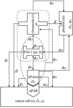
(8)Fig. 1. Schematic overview of the modelled mechanism, evidencing the parameters involved as introduced in the text. 3. The numerical technique
Eqs.(4)–(8) constitute a system of five coupled PDEs modelling the interaction between the uPA system and the cancer cells, to be solved over a one-dimensional spatial domain. The problem can be tackled using the equidistribution principle [46–50], by means of which the FEM discretization is controlled equidistributing in each subinterval of Ω a monitor function [51,52]. It results a quite efficient method allowing for extremely accurate representations of sharp solution features, such as shocks or defects, while the optimal choice of the monitor function depends on the problem being solved, the numerical discretization being used, and the norm of the error that is to be minimized [51].
Denoting by
w(
x,
t)
a solution over a physical domainΩp= [
0,
1]
of a PDE system, with x the physical coordinate, weintroduce a fixed computational domainΩc
= [
0,
1]
withξ
computational coordinate, defining a coordinate transformationrepresenting a one-to-one mapping at time t from computational spaceΩc
×
(
0,
T]
to physical spaceΩp×
(
0,
T]
x
=
x(ξ,
t), ξ ∈
Ωc,
t∈
(
0,
T]
(9)and the reverse
ξ = ξ(
x,
t),
x∈
Ωp,
t∈
(
0,
T]
(10)from physical spaceΩp
×
(
0,
T]
to computational spaceΩc×
(
0,
T]
holds. A uniform gridξ
i=
i/
N,
i=
0,
1, . . . ,
N (11)imposed on computational space, corresponds to a set of nodes on physical space
0
=
x0(
t) <
x1(
t) < · · ·
xN(
t) =
1.
(12)A mesh equidistributes a monitor function M
(w(
x,
t))
in each subinterval ofΩif
xi(t) xi−1(t) M(w(
s,
t))
ds=
1 N
1 0 M(w(
s,
t))
ds (13)and generalizing over the integration domain, we obtain the integral form of the equidistribution principle
x(ξ,t) 0 M(w(
s,
t))
ds=
ξ
1 0 M(w(
s,
t))
ds.
(14)Differentiating(14)with respect to
ξ
, the mesh equation is obtained, allowing to determine the coordinate mapping x(ξ,
t)
M(
x(ξ,
t))
∂
∂ξ
x(ξ,
t) =
1 0 M(w(
s,
t))
ds=
C(
t)
(15)and in order to keep constant the equidistribution of the monitor function over the integration domain, at a larger monitor function value corresponds a denser mesh.
We have demonstrated [42] that the monitor function introduced by Beckett et al. [50], based on the method proposed by Huang et al. [53] ensures a good quality control of the mesh and the final convergence of the FEM solution [50,51], and therefore we choose M
(w(
x,
t)) =
1 0
∂w(
x,
t)
∂
x
1/2 dx+
∂w(
x,
t)
∂
x
1/2.
(16)We are in presence of a multidimensional time-dependent problem, which FEM discretization is done via the method of lines; the overall adaptive solution process involves an iteration in which: (i) a mesh is generated using the equidistribution principle based on the numerical solution at the current time step; (ii) the PDEs are solved on the new generated grid and then updated in time. The stability of the iterative updating relies on a proper selection of the updating time step∆t [54], at which our PDE system, Eqs.(4)–(8), is numerically solved using FEM. To overcome the difficulty related to the non-linearity we used Galerkin’s method associated to a weak formulation of the residual of the differential equations [40], discretizing them in time via an implicit Euler method, and interpolating the local distribution in each element of our variables by quadratic shape functions. Major details can be found in [42] and references therein. We point out that, since our problem is modelled by five coupled PDEs solved simultaneously, at each time step we have five unknown exact solutions
w(
z,
t)
, one for each of the monitored species. The used multi-pass algorithm is:a uniform initial grid xj
(
0)
is generated and the corresponding initial solutionw
j(
0)
is calculated using FEM;a temporal loop is done in the time domain updating mesh and solution w, putting forward PDEs:
while tn
<
Tthe mesh is redistributed in a few steps
v ≥
0:do
the monitor function is evaluated at the current time step, the grid is moved from xj
(v)
to xj(v+
1) equidistributingthe monitor function in each subinterval and a solution
w
j(v +
1) is calculated on the new mesh, for each of thefive coupled equations (4)–(8).
until
v ≤ v
maxthe PDE system is put forward on the new mesh xj
(v +
1)
to obtain a numerical approximationw
j(v +
1)
at the newtime level tn+1. end
For computational convenience, we adopt the non-dimensional system, hence default set of model parameters, boundary and initial conditions as in [33] for the one dimensional domain: consequently, distance is rescaled with L
=
0.
1 cm, a distance of cancer cells at early stage of invasion; if D=
1×
10−6cm2s−1is a representative chemical diffusion coefficient,time is rescaled with
τ =
L2D−1, while the reference concentration values for the dependent variables are c0
=
6.
7×
107cell cm−3,
v
0=
1 nM,
u0=
1 nM,
p0=
1 nM,
m0=
0.
1 nM. Finally, the complete set of the non-dimensional parameters isdeduced: Dc
=
3.
5×
10−4,
Du=
2.
5×
10−3,
Dp=
3.
5×
10−3,
Dm=
4.
91×
10−3, χ
u=
3.
05×
10−2, χ
p=
3.
75×
10−2, χ
v=
2
.
85×
10−2, µ
1=
0.
25, µ
2=
0.
15, α
31=
0.
215, α
41=
0.
5, δ =
8.
15, φ
21=
0.
75, φ
22=
0.
55, φ
31=
0.
75, φ
33=
0
.
3, φ
41=
0.
75, φ
42=
0.
55, φ
52=
0.
11, φ
53=
0.
75, φ
54=
0.
5. Moreover, for x∈
Ω,
ifε =
0.
01, the imposed initialconditions are c
(
x,
0) =
exp(−|
x|
2ε
−1), v(
x,
0) =
1−
0.
5c(
x,
0),
u(
x,
0) =
0.
5c(
x,
0),
p(
x,
0) =
0.
05c(
x,
0),
m(
x,
0) =
0 [32,33]. Such conditions, at x
=
0, allow the presence of a cluster of cancer cells, while the remaining portion of the domain is filled by ECM; the initial concentrations of uPA and PAI-1 are proportional to the cancer cells concentration while plasmin is not yet produced. Further, all the components remain confined within the simulated portion of tissue, thus the PDEs system satisfies zero-flux boundary conditions, with the exception of the ordinary differential equation(5).Facing the kind of problems we treat, a difficulty is often the lack of experimental determinations of the biological parameters involved. In this respect, an instructive discussion is given in [32]: most of the parameters available in the literature are not univocally determined, having estimates falling in ranges, on average, two order of magnitude wide; otherwise, they are estimated by numerical simulations on the grounds of agreement with experimental results, if available. Consequently, any numerical or experimental parameter errors at this stage is not relevant being adsorbed in the relative estimate range and possible error effects are not considered. In [33] the authors have been performed both linear stability and parameters sensitivity analyses, showing that variations of some key parameter can change the qualitative character of the solution, leading to different invasion pattern by cancer cells; on the contrary, these latter do not seem appreciably affected by slight fluctuations of the parameters around some average values. In particular, depending on the diffusion coefficient for cancer cells Dc, either homogeneous or heterogeneous proliferation can arise, which we tune using the parameter set
tested in [33].
For our computations, we modelled the real problem simulating a one-dimensional portion of tissue of thickness
Fig. 2. Nodes trajectories versus time for the adaptive mesh algorithm in the 0≤x≤7 spatial domain and in the 0≤t≤500 time interval where only one grid point trajectory every twenty has been included; the horizontal and vertical axes correspond to the tissue thickness and the time scale of the solution evolution, respectively.
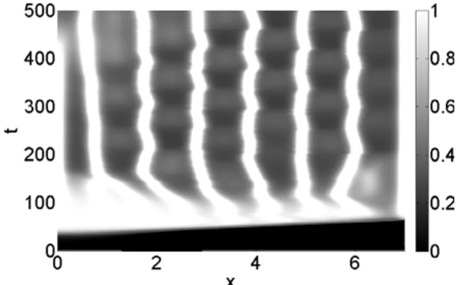
Fig. 3. Surface contour plots of the cancer cells concentration evolution in the 0≤x≤7 spatial domain and in the 0≤t≤500 time interval, imposing a random motility value Dc =3.5×10⁻⁴; the concentration is linearly mapped in a grey levels scale between the black (zero concentration) and white (maximum concentration) colours.
and the dynamical evolution of the system is monitored in the 0
<
t<
500 non-dimensional time interval, corresponding to about 58 days, with steps of size dt=
0.
5. We remember that both the dimensional timescale and the tissue thickness can be recovered multiplying, respectively, t byτ
, and x by L. Besides Dc=
3.
5×
10−4, we performed our simulation alsofor Dc
=
4.
25×
10−3. Eqs.(4)–(8)are solved at each time step, replacing in Eq.(16)the exact solutionw(
x,
t)
with c(
x,
t)
,allowing the grid points on which the solution is computed to be driven by the cancer cell concentration. Such choice gives a denser mesh according to growing
∇
c.4. Numerical results and discussion
InFig. 2, we show the node trajectories generated by the adaptive mesh algorithm inside the simulated domain, tracing only one grid point trajectory every twenty for plotting convenience. The parameters introduced in the previous section have been used, in particular a random motility for cancer cells Dc
=
3.
5×
10−4. The horizontal axis corresponds to thetissue thickness in the 0
≤
x≤
7 range, while the vertical axis corresponds to the time scale of the solution evolution in the 0≤
t≤
500 time interval. At t=
0 the nodes are uniformly spaced and the cell distribution is prescribed by the initial conditions; for t>
0 the nodes move according to the evolution of∇
c: their trajectories are smooth within few tenth oftime unit, while above t
=
40 they become more and more inhomogeneous. Such behaviour reflects inFig. 3, where we show the proliferation pattern of cancer cells, linearly mapped in a grey level scale between the black (zero density) and white (maximum density) colours, with horizontal and vertical axes as inFig. 2. For t<
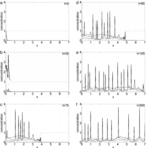
40, no proliferation can be de-tected along the tissue thickness, while at increasing times cancer cells start to proliferate, building a branched and strongly inhomogeneous spatio-temporal pattern, a behaviour which is in agreement with the results of Andasari et al. [33].InFig. 4(a)–(f) we monitor the density evolution of the interacting species along the tissue thickness, at various temporal steps, i.e. the cancer cells density c
(
x,
t)
(solid line), the VN densityv(
x,
t)
(dotted line), the uPA density u(
x,
t)
(dash-dotted line), the PAI-1 density p(
x,
t)
(dashed line) and the plasmin density m(
x,
t)
(thin dash-dotted line). The horizontal axis corresponds to the tissue thickness in the 0≤
x≤
7 range, while the vertical axis corresponds to the concentration of the chemical species. We focus our attention on the cancer cell concentration profile: at t=
0,Fig. 4(a), it is prescribed by the imposed initial conditions, and up to t=
30 it is uniformly clustered close x=
0 in a progressively broad and smooth structure. At t=
35,Fig. 4(b), the density profile starts to change: around x=
0.
5 a steep and sharp front of invasion isFig. 4. Plot of the concentration evolution of the different species in the simulated domain, imposing a random motility value Dc =3.5×10⁻⁴: solid line, cancer cells c; dotted line, vitronectinv; dash-dotted line, uPA u; dashed line, PAI-1 p; dash-dotted thin line, plasmin m. Each panel corresponds to a snapshot taken during the time evolution: t=0 (a), t=35 (b), t=75 (c), t=85 (d), t=105 (e), t=500 (f). The upper plot in panel (b) corresponds to the eight-fold magnification of the cancer cell profile c, in the 0≤x≤0.5 range.
present, preceded by a broad structure, both exhibiting an indented fine structure as evidenced in the eight fold magnified upper plot of the cancer cells density c
(
x,
t)
in the 0≤
x≤
0.
5 range; at the same time, the other chemical densities evolve too, in particular the VN degrades, as a consequence of the interaction of cancer cells with the uPA system. Fort
=
75,Fig. 4(c), new and sharp structures arise in the density profile superimposed on a smooth background, indicating an inhomogeneous cancer cell clustering. In this case, the indented invading front has penetrated about x=
4, a smaller portion of tissue with respect to the predictions in Ref. [33] where, for the same time interval, the front of invasion is around x=
5; in our simulation, instead, such degree of invasion is reached for t=
85, seeFig. 4(d). At t=
105,Fig. 4(e), the simulated domain is almost entirely invaded, a behaviour persisting up to t=
500,Fig. 4(f): the density profile presents repeated sharp peaks, consequence of the inhomogeneous character of the cancer cell clusters, hence malignancy [24]. Besides the overall agreement of our simulations with that showed in Ref. [33], our method allows capturing some fine structures not observed otherwise: in fact, during the cancer cell invasion, the invading front is always characterized by an irregular and spiky structure, at the boundary between cancer ad healthy cells.Considering now the effect of an increase in cancer cell motility, as a consequence of mutations giving to cancer cells an increased degree of malignancy, inFig. 5we show the surface plot of the cancer cells density in the simulated spatio-temporal domain obtained imposing Dc
=
4.
25×
10−3; once again, below t=
40 no proliferation can be detected; forFig. 5. Surface contour plots of the cancer cells concentration evolution in the 0≤x≤7 spatial domain and in the 0≤t≤500 time interval, imposing a random motility value Dc=4.25×10⁻³; the concentration is linearly mapped in a grey levels scale between the black (zero concentration) and white (maximum concentration) colours.
t
>
40, the cancer cell concentration grows uniformly along the tissue thickness, and above t=
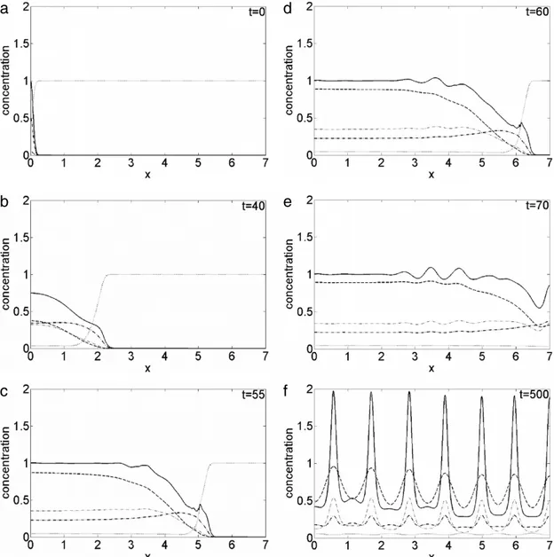
100 the proliferation pattern exhibits an inhomogeneous evolution characterized by quite regularly spaced branches protruding in time.Nevertheless, snapshots of the chemicals density taken at selected times give us a dynamical evolution smoother and faster than in the case with Dc
=
3.
5×
10−4, seeFig. 6. In fact, at t=
0,Fig. 6(a), the cancer cell concentration profileis still prescribed by the initial conditions imposed. At t
=
40 a steep and smooth front of invading cells is present nearx
=
2.
3,Fig. 6(b), which for t=
55 moves to x=
5.
5, with an irregular fine structure superimposed,Fig. 6(c). For t=
60 the invading front is around x=
6.
5 and new structures start to grow in the cancer cell concentration profile,Fig. 6(d); att
=
70,Fig. 6(e), the tumour has penetrated the entire simulated domain, while the cancer cell clusters are clearly visible over the smooth background. Finally, at t=
500,Fig. 6(f), the density profile presents sharp and quite regularly spaced clusters corresponding to the branches ofFig. 5.Once again, the dynamical density profile of the species present in the simulated domain, obtained using the adaptive grid, is in agreement with that computed in Ref. [33], whoseFigs. 4
(
t=
75)
and6(
Dn=
0.
00425)
can be compared to ours4(c) and (e). Apart from slight discrepancies arising regarding the speed of propagation of the invading front, our results indicate that, imposing a motility value Dc
=
3.
5×
10−4, the invasion proceeds at a lower speed, on the contrary with avalue of Dc
=
4.
25×
10−3. Further, from the comparison ofFigs. 4and6we observe that an increase of the cancer cellmotility causes an obvious increase in the speed of invasion; not obvious, instead, is the irregular and spiky density profile at the boundary between cancer and healthy cells, a behaviour which can be associated to the border irregularity of tumour clusters, a hallmark of malignancy. Also intriguing appears the smoothness of the profiles shown inFig. 6, compared to that ofFig. 4: in fact, it seems that on going towards malignant mutations of cancer cells characterized by higher Dcvalues, the
irregularity of the invasion front diminishes while increasing its propagation speed, thus suggesting that a reduced border irregularity of the tumour cluster is compensated by an increased speed of invasion of the healthy tissue. Once the invasion is completed,Figs. 4(f) and6(f), the cancer cell density profile shows the sharp features associated to the inhomogeneous spatio-temporal proliferation pattern ofFigs. 3and5, respectively, even if at higher Dc,Fig. 6(f), they appear regularly spaced.
A study performed on a one-dimensional test problem [55], in particular on a spatial region of thickness 10
µ
m discretized via both uniform and adaptive grids with 256 grid points, puts in evidence that in the case of the adaptive grid, with respect to the uniform one, minimum grid size and numerical error are, respectively, three order of magnitude and one order of magnitude smaller; moreover, given a required tolerance, the computational cost is always smaller for the adaptive grid. As we have demonstrated [42] that the used monitor function results in a more reliable, effective and efficient method than that used in [55], an overall improvement of our MMPDE method is expected, particularly with respect to uniform grids methods, and suggest that during the early stage of tumour formation a high degree of malignancy is associated to a low speed of invasion; once a portion of tissue has been invaded by tumour, malignancy rely on the highly non homogeneous proliferation patterns, seeFig. 3. On the other hand, mutations leading to an increased cell motility are associated to a faster but smoother density dynamics: as before, once a portion of tissue has been invaded by tumour, the inhomogeneous proliferation patterns shown inFig. 4characterize an overall malignancy of the cancer proliferation.5. Conclusions
In this work, we have implemented the MMPDE numerical technique using FEM, in order to solve the PDE system derived by Andasari et al. [33], as arising from a mathematical modelling of the interaction of the uPA system with cancer cell proliferation. Variations in cancer cell motility as a consequence of malignant cell mutations lead to increased speed of the invasion front. Although the present work deal with a somewhat simplified 1D model problem, the obtained numerical results confirm the validity of the used technique; moreover, due to the improved spatial resolution provided with respect to computations performed on uniformly discretized domains, add more realistic predictions about the early stage of tumour
Fig. 6. Plot of the concentration evolution of the different species in the simulated domain, imposing a random motility value Dc =4.25×10⁻³: solid line, cancer cells c; dotted line, vitronectinv; dash-dotted line, uPA u; dashed line, PAI-1 p; dash-dotted thin line, plasmin m. Each panel corresponds to a snapshot taken during the time evolution: t=0 (a), t=40 (b), t=55 (c), t=60 (d), t=70 (e), t=500 (f).
dynamics. In fact, at low Dcvalues, our simulations put in evidence a fine and irregular structure of the tumour invading
front which can be associated to an increased degree of malignancy; a higher motility value causes an increase in the invasion speed with a smoothing of the invasion front, thus evidencing the interplay between cancer cells motility and their heterogeneous proliferation. We believe such predictions can be useful from a clinical and surgical point of view, and work is in progress to include in the model the effect of nutrients like oxygen and/or glucose, as well as extension in two and three dimensions.
References
[1]L. Preziosi, Modelling tumour growth and progression, in: A. Buikis, R. Ciegis, A.D. Fitt (Eds.), Progress in Industrial Mathematics at ECMI 2002, Springer, Berlin, 2004, pp. 53–66.
[2]P. Macklin, S. McDougall, A.R.A. Anderson, M.A.J. Chaplain, V. Cristini, J. Lowengrub, Multiscale modelling and nonlinear simulation of vascular tumour growth, J. Math. Biol. 58 (2009) 765–798.
[3]L. Preziosi, A.R. Tosin, Multiphase modeling of tumor growth and extra cellular matrix interaction: mathematical tools and applications, J. Math. Biol. 58 (2009) 625–656.
[4]D. Ambrosi, L. Preziosi, On the closure of mass balance models for tumour growth, Math. Models Methods Appl. Sci. 12 (2002) 737–754.
[5]H.M. Byrne, Modelling avascular tumor growth, in: L. Preziosi (Ed.), Cancer Modelling and Simulation, Chapman & Hall/CRC Press, Boca Raton, 2003, pp. 75–120.
[6] H. Byrne, L. Preziosi, Modelling solid tumour growth using the theory of mixtures, Math. Med. Biol. 20 (2003) 341–366.
[7] M.A.J. Chaplain, M. Ganesh, I.G. Graham, Spatio-temporal pattern formation on spherical surfaces: numerical simulation and application to solid tumour growth, J. Math. Biol. 42 (2001) 387–423.
[8] J.A. Sherratt, M.A.J. Chaplain, A new mathematical model for avascular tumour growth, J. Math. Biol. 43 (2001) 291–312.
[9] C.J.W. Breward, H.M. Byrne, C.E. Lewis, Modeling the interactions between tumour cells and a blood vessel in a microenvironment within a vascular tumour, Eur. J. Appl. Math. 12 (2001) 529–556.
[10]D. Ambrosi, F. Mollica, On the mechanics of a growing tumor, Internat. J. Engrg. Sci. 40 (2002) 1297–1316.
[11]C.Y. Chen, H.M. Byrne, J.R. King, The influence of growth-induced stress from the surrounding medium on the development of multicell spheroids, J. Math. Biol. 43 (2001) 191–220.
[12]A.R.A. Anderson, M.A.J. Chaplain, Continuous and discrete mathematical models of tumour-induced angiogenesis, Bull. Math. Biol. 60 (1998) 857–899. [13]H. Levine, S. Pamuk, B. Sleeman, M. Nilsen-Hamilton, Mathematical modeling of capillary formation and development in tumor angiogenesis:
penetration into the stroma, Bull. Math. Biol. 63 (2001) 801–863.
[14]H.A. Levine, B.D. Sleeman, Modelling tumour induced angiogenesis, in: L. Preziosi (Ed.), Cancer Modelling and Simulation, Chapman & Hall/CRC Press, Boca Raton, 2003, pp. 147–184.
[15]S.R. McDougall, A.R.A Anderson, M.A.J Chaplain, J.A. Sherratt, Mathematical modelling of flow through vascular networks: implications for tumor induced angiogenesis and chemotherapy strategies, Bull. Math. Biol. 64 (2002) 673–702.
[16]S.R. McDougall, A.R.A. Anderson, M.A.J. Chaplain, Mathematical modelling of dynamic adaptive tumour-induced angiogenesis: clinical implications and therapeutic targeting strategies, J. Theoret. Biol. 241 (2006) 564–589.
[17]J. Folkman, Tumor angiogenesis, Adv. Cancer Res. 19 (1974) 331–358. [18]J. Folkman, The vascularization of tumors, Sci. Am. 234 (1976) 58–73. [19]J. Folkman, M. Klagsbrun, Angiogenic factors, Science 235 (1987) 442–447. [20]D. Hanahan, R.A. Weinberg, The hallmarks of cancer, Cell 100 (2000) 57–70.
[21]M.A.J. Chaplain, A.R.A. Anderson, Mathematical modelling of tissue invasion, in: L. Preziosi (Ed.), Cancer Modelling and Simulation, Chapman & Hall/CRC Press, Boca Raton, 2003, pp. 269–298.
[22]A.R.A. Anderson, M.A.J. Chaplain, E.L. Newman, R.J. Steele, A.M. Thompson, Mathematical modeling of tumour invasion and metastasis, J. Theor. Med. 2 (2000) 129–154.
[23]L. Preziosi (Ed.), Cancer Modelling and Simulation, Chapman & Hall/CRC Press, Boca Raton, 2003.
[24]R.P. Araujo, D.L.S. McElwain, A history of the study of solid tumour growth: the contribution of mathematical modeling, Bull. Math. Biol. 66 (2004) 1039–1091.
[25]S. Astanin, L. Preziosi, Multiphase models of tumour growth, in: N. Bellomo, M. Chaplain, E. De Angelis (Eds.), Selected Topics in Cancer Modelling: Genesis, Evolution, Immune Competition, and Therapy, Birkhauser, Boston, 2008, pp. 223–254.
[26]L. Graziano, L. Preziosi, Mechanics in tumour growth, in: F. Mollica, L. Preziosi, K.R. Rajagopal (Eds.), Modeling of Biological Materials, Birkhauser, Boston, 2007, pp. 263–322.
[27]T. Roose, S.J. Chapman, P.K. Maini, Mathematical models of avascular tumor growth, SIAM Rev. 49 (2007) 179–208. [28]P. Tracqui, Biophysical models of tumour growth, Rep. Progr. Phys. 72 (2009) 056701–056731.
[29]J.S. Lowengrub, H.B. Frieboes, F. Jin, Y.L. Chuang, X. Li, P. Macklin, S.M. Wise, V. Cristini, Nonlinear modelling of cancer: bridging the gap between cells and tumours, Nonlinearity 23 (2010) R1–R91.
[30]M.E. Hubbard, H.M. Byrne, Multiphase modeling of vascular tumour growth in two spatial dimensions, J. Theoret. Biol. 316 (2013) 70–89.
[31]A. Gerisch, M.A.J. Chaplain, Mathematical modelling of cancer cell invasion of tissue: local and nonlocal models and the effect of adhesion, J. Theoret. Biol. 250 (2008) 684–704.
[32]M.A.J. Chaplain, G. Lolas, Mathematical modelling of cancer cell invasion of tissue: the role of the urokinase plasminogen activation system, Math. Models Methods Appl. Sci. 15 (2005) 1685–1734.
[33]V. Andasari, A. Gerisch, G. Lolas, A.P. South, M.A.J. Chaplain, Mathematical modeling of cancer cell invasion of tissue: biological insight from mathematical analysis and computational simulation, J. Math. Biol. 63 (2011) 141–171.
[34]P.A. Andreasen, L. Kjøller, L. Christensen, M.J. Duffy, The urokinase-type plasminogen activator system in cancer metastasis: a review, Int. J. Cancer 72 (1997) 1–22.
[35] P.A. Andreasen, R. Egelund, H.H. Petersen, The plasminogen activation system in tumor growth, invasion, and metastasis, Cell. Mol. Life Sci. 57 (2000) 25–40.http://dx.doi.org/10.1007/s000180050497.
[36] M.L. Nyström, G.J. Thomas, M. Stone, I.C. Mackenzie, I.R. Hart, J.F. Marshall, Development of a quantitative method to analyse tumour cell invasion in organotypic culture, J. Pathol. 205 (2005) 468–475.http://dx.doi.org/10.1002/path.1716.
[37] V.L. Martins, J.J. Vyas, M. Chen, K. Purdie, C.A. Mein, A.P. South, A. Storey, J.A. McGrath, E.A. O’Toole, Increased invasive behavior in cutaneous squamous cell carcinoma with loss of basement-membrane type VII collagen, J. Cell. Sci. 122 (2009) 1788–1799.http://dx.doi.org/10.1242/jcs.042895. [38]V. Cristini, X. Li, J.S. Lowengrub, S.M. Wise, Nonlinear simulations of solid tumor growth using a mixture model: invasion and branching, J. Math. Biol.
58 (2009) 723–763.
[39]S.M. Wise, J.S. Lowengrub, V. Cristini, An adaptive multigrid algorithm for simulating solid tumour growth using mixture models, Math. Comput. Modelling 53 (2011) 1–20.
[40]O.C. Zienkiewicz, R.L. Taylor, The Finite Element Method, fifth ed., Butterworth–Heinemann, Oxford, 2002. [41]T. Tang, Moving mesh methods for computational fluid dynamics, Contemp. Math. 383 (2005) 141–173.
[42]A. Amoddeo, R. Barberi, G. Lombardo, Moving mesh partial differential equations to describe nematic order dynamics, Comput. Math. Appl. 60 (2010) 2239–2252.
[43]A. Amoddeo, R. Barberi, G. Lombardo, Electric field-induced fast nematic order dynamics, Liq. Cryst. 38 (2011) 93–103.
[44]A. Amoddeo, R. Barberi, G. Lombardo, Surface and bulk contributions to nematic order reconstruction, Phys. Rev. E 85 (2012) 061705–061705-10. [45] A. Amoddeo, R. Barberi, G. Lombardo, Nematic order and phase transition dynamics under intense electric fields, Liq. Cryst. 40 (2013) 799–809.
http://dx.doi.org/10.1080/02678292.2013.783133.
[46]C. de Boor, in: J. Morris (Ed.), Good Approximation by Splines with Variable Knots II, in: Lecture Notes in Mathematics, vol. 263, Springer-Verlag, Berlin, 1974, pp. 12–20.
[47]V. Pereyra, E.G. Sewell, Mesh selection for discrete solution of boundary problems in ordinary differential equations, Numer. Math. 23 (1975) 261–268. [48]R.D. Russell, J. Christiansen, Adaptive mesh selection strategies for boundary value problems, SIAM J. Numer. Anal. 15 (1978) 59–80.
[49]A.B. White, On selection of equidistributing meshes for two-point boundary-value problems, SIAM J. Numer. Anal. 16 (1979) 472–502.
[50]G. Beckett, J.A. Mackenzie, A. Ramage, D.M. Sloan, On the numerical solution of one-dimensional PDEs using adaptive methods based on equidistribution, J. Comput. Phys. 167 (2001) 372–392.
[51]G. Beckett, J.A. Mackenzie, Convergence analysis of finite difference approximations on equidistributed grids to a singularly perturbed boundary value problem, Appl. Numer. Math. 35 (2000) 87–109.
[52]W. Huang, Practical aspects of formulation and solution of moving mesh partial differential equations, J. Comput. Phys. 171 (2001) 753–775. [53]W. Huang, Y. Ren, R.D. Russell, Moving mesh partial differential equations (MMPDEs) based upon the equidistribution principle, SIAM J. Numer. Anal.
31 (1994) 709–730.
[54]J. Anderson, C. Titus, P. Watson, P. Bos, Significant speed and stability increases in multi-dimensional director simulations, SID Digest 31 (2000) 906–909.
[55]A. Ramage, C.J.P. Newton, Adaptive grid methods for Q-tensor theory of liquid crystals: a one-dimensional feasibility study, Mol. Cryst. Liq. Cryst. 480 (2008) 160–181.