This content has been downloaded from IOPscience. Please scroll down to see the full text.
Download details:
IP Address: 193.204.8.28
This content was downloaded on 20/10/2015 at 08:03
Please note that terms and conditions apply.
Generation and detection of large and robust entanglement between two different mechanical
resonators in cavity optomechanics
View the table of contents for this issue, or go to the journal homepage for more 2015 New J. Phys. 17 103037
PAPER
Generation and detection of large and robust entanglement between
two different mechanical resonators in cavity optomechanics
J Li1,2,3
, I Moaddel Haghighi1,2
, N Malossi1,2
, S Zippilli1,2
and D Vitali1,2
1 School of Science and Technology, Physics Division, University of Camerino, via Madonna delle Carceri, 9, I-62032 Camerino(MC), Italy 2 INFN, Sezione di Perugia, Italy
3 Author to whom any correspondence should be addressed.
E-mail:[email protected]
Keywords: cavity optomechanics, mechanical entanglement, quantum open systems
Abstract
We investigate a general scheme for generating, either dynamically or in the steady state, continuous
variable entanglement between two mechanical resonators with different frequencies. We employ an
optomechanical system in which a single optical cavity mode driven by a suitably chosen two-tone
field is coupled to the two resonators. Significantly large mechanical entanglement can be achieved,
which is extremely robust with respect to temperature.
1. Introduction
Entanglement is the distinguishing feature of quantum mechanics and is the physical phenomenon according to which only the properties of the entire system have precise values, while the physical properties of a subsystem can be assigned only in reference to those of the other ones. It is now intensively studied because it corresponds to peculiar nonlocal correlations which allows performing communication and computation tasks with an efficiency which is not achievable classically [1].
Furthermore, for a deeper understanding of the boundary between the classical and quantum world, it is important to investigate up to which macroscopic scale one can observe quantum behavior, and in particular under which conditions entanglement between macroscopic objects, each containing a large number of the constituents, can arise. Entanglement between two atomic ensembles has been successfully demonstrated in[2],
while entanglement between two Josephson-junction qubits has been detected in[3,4]. More recently,
macroscopic entanglement has been demonstrated in electro-mechanical systems[5]: continuous variable (CV)
entanglement, similar to that considered by Einstein–Podolski and Rosen (EPR) [6], has been generated and
detected between the position and momentum of a vibrational mode of a 15μm diameter Al membrane, and the quadratures of a microwave cavityfield, following the theory proposal of [7].
Entanglement between two mechanical resonators(MRs) has been instead demonstrated only at the microscopic level, in the case of two trapped ions[8], and between two single-phonon excitations in
nano-diamonds[9]. The realization of this kind of entanglement at the more macroscopic level of micromechanical
resonators would be extremely important both for practical and fundamental reasons. In fact, on the one hand, entangled MRs at distant sites could represent an important building block for the implementation of quantum networks for long-distance routing of quantum information[10]; on the other hand, these nonclassical states
represent an ideal playground for investigating and comparing decoherence theories and modifications of quantum mechanics at the macroscopic level[11–13].
Many different schemes have been proposed in the literature for entangling two MRs, especially exploiting optomechanical and electromechanical devices[14,15], in which the two MRs simultaneously interact with one
or more electromagnetic cavityfields. References [16–18] considered the steady state of different systems of
driven cavities:[16] focused on two mirrors of a ring cavity, while [17] assumed to drive two independent linear
cavities with two-mode squeezed light transferring its entanglement to the cavity end-mirrors[18] instead
considered a double-cavity scheme in which one cavity couples to the relative motion of two MRs, and the OPEN ACCESS
RECEIVED
10 June 2015
REVISED
21 August 2015
ACCEPTED FOR PUBLICATION
25 September 2015
PUBLISHED
19 October 2015 Content from this work may be used under the terms of theCreative Commons Attribution 3.0 licence.
Any further distribution of this work must maintain attribution to the author(s) and the title of the work, journal citation and DOI.
second cavity to their center-of-mass; when the system is appropriately driven by squeezed light, such squeezing is transferred to the two MRs which are then prepared in a stationary EPR-like state. Actually, steady-state entanglement can be achieved, even if at a smaller value, also without squeezed driving, either between two movable mirrors in a Fabry–Perot cavity [19], between two mechanical modes of a single movable mirror [20],
or in the case of two semi-transparent membranes interacting with two driven cavity modes[21].
A different approach for generating entangled MRs exploits conditional measurements on light modes entangled or correlated with mechanical degrees of freedom[22–27]. In this case, entanglement is generated at
the measurement and it has afinite lifetime which may be severely limited by the interaction of the MRs with their reservoirs. A similar strategy has been provided to enhance the entanglement of two MRs[28]. More recent
proposal applied reservoir engineering ideas[29–33] to optomechanical scenarios, by exploiting suitable
multi-frequency drivings and optical architectures in order to achieve more robust generation of steady state entanglement between two MRs[34–40], eventually profiting from mechanical nonlinearities and/or
parametric driving[41,42].
In the present paper we propose a novel optomechanical/electromechanical scheme for the generation of remarkably large CV entanglement between two MRs with different frequencies, which is also extremely robust with respect to thermal noise. The scheme is particularly simple, involving only a single, bichromatically-driven, optical cavity mode, and optimally works in a rotating wave approximation(RWA) regime where counter-rotating, non-resonant, terms associated with the bichromatic driving are negligible. The scheme shares some analogies with the reservoir-engineering schemes of[34,36,38,40], but it may be used to generate robust
entanglement also in a pulsed regime, in the special case of equal effective couplings at the two sidebands, where the system becomes analogous to the Sørensen–Mølmer scheme for entangling trapped ions in a thermal environment[43]. This latter scheme has been already considered in an optomechanical scenario by Kuzyk et al
[44] for entangling dynamically two optical modes via their common interaction with a single MR.
The paper is organized as follows. In section2we derive the effective quantum Langevin equations(QLEs) describing the dynamics of the system in the RWA. In section3we solve the dynamics in terms of the mechanical Bogoliubov modes of the system[34,36,45], derive the steady state of the system in the stable case, and provide
simple analytical expressions for the achievable mechanical entanglement, showing its remarkable robustness with respect to temperature. In section4we instead consider the special case of equal couplings, when the system can be mapped to the Sørensen–Mølmer scheme [43], in which mechanical entanglement is generated only
dynamically and slowly decays to zero at long times. In section5we solve and discuss the exact dynamics of the system in order to establish the conditions under which the RWA does not seriously affect the robust generation of large mechanical entanglement. In section6we discuss the experimental detection of such entanglement and present some concluding remarks. In the appendices we provide some detail on the dynamical evolution of the system, and present a careful derivation of the linearized QLE in the RWA regime.
2. System Hamiltonian and derivation of the effective Langevin equations
As shown infigure1, we consider an optical cavity mode with resonance frequencyωcand annihilation operator
aˆ interacting via the usual optomechanical interaction with two different MRs, with frequenciesω1andω2and annihilation operators bˆ and1 bˆ2respectively. The cavity mode is bichromatically driven at the two frequencies
ω0+ ω1andω0− ω2, with the reference frequencyω0detuned from the cavity resonance by a quantityΔ0= ωc− ω0. If we describe the cavityfield in a reference frame rotating at the frequency ω0, then the system Hamiltonian is given by H b b b b a a g b b g b b a a Ee t E e t a h.c. . 1 1 1 1 2 2 2 0 1 1 1 2 2 2 1 i 1 2 i 2
(
)
(
)
(
)
ˆ ˆ ˆ ˆ ˆ ˆ ˆ ˆ ˆ ˆ ˆ ˆ ˆ ˆ ( ) † † † † † † † ⎡ ⎣⎢ ⎤⎦⎥ ⎡ ⎣ ⎤⎦ w w = + + D + + + + + -w + w +This means that the cavity mode is simultaneously driven on the blue sideband associated with the MR with annihilation operatorb ,ˆ1and on the red sideband associated with the MR withb .ˆ2 The nonzero detuningΔ0 makes the present scheme different from the one studied in the supplementary material of[34] which restricts to
the resonant caseΔ0= 0. Our model is instead related to the scheme proposed by Kuzyk et al [44] for entangling dynamically two optical modes via their common interaction with a single MR: here we will dynamically entangle two MRs via their common interaction with an optical mode.
The system dynamics can be efficiently studied by linearizing the optomechanical interaction in the limit of large drivingfield. In this case the average fields for both cavity, α(t), and mechanical degrees of freedom, βj(t), are large, and one can simplify the interaction Hamiltonian at lowest order in thefield fluctuations
a t a t t b t b t t , . 2 j j j ˆ ( ) ˆ ( ) ( ) ˆ ( ) ˆ ( ) ( ) ( ) d a d b = -=
-Differently from the typical optomechanical settings in which the steady state averagefields are
time-independent, here the bichromatic driving induces a time-dependent, periodic steady state averagefield which, in turn, implies time-dependent effective coupling strengths for the linearized dynamics of thefluctuations. As originally discussed in[46], and detailed in appendixB, approximated dynamical equations for thefluctuation operatorsda tˆ ( )and b tdˆ ( )j can be derived, in the interaction picture with respect to the Hamiltonian
Hˆ0 ( 1 1b bˆ ˆ1 2 2b b ,ˆ ˆ )2
† †
w w
= + by neglecting the non-resonant/time-dependent components of the effective
linearized interactions. It is possible to prove that this approach is justified when (see equation (B.21))
gj Ej , , . 3
j
j 1 2 ( )
w kw w -w
The corresponding QLE including thermal noise and dissipation at ratesκ and γjfor the cavity and the mechanical mode jÎ1, 2respectively, are
aˆ˙ ( i ) ˆa iG b1 ˆ1 iG b2 ˆ2 2 aˆin, ( )4 † d = - k+ D d - d - d + k b b G a b 2 i , 5 1 1 1 1 1 1 in ˆ˙ ˆ ˆ† ˆ ( ) d = -g d - d + g b b G a b 2 i , 6 2 2 2 2 2 2 in ˆ˙ ˆ * ˆ ˆ ( ) d = -g d - d + g where G g E G g E i , i , 7 1 1 1 1 2 2 2 2 ( ) w k w k = - D + = + D
-are the(generally complex) linear optomechanical couplings, and aˆ and bin
j
in
ˆ are standard input noise operators with zero mean, whose only nonzero correlation functions are aˆ ( ) ˆ ( )in t ain t¢† =d(t- ¢ , b t b tt)
j j in in ˆ ( ) ˆ ( )¢† nj 1 t t ( ¯ ) (d ) = + - ¢ and b t b tj j nj t t , in in ˆ ( ) ˆ ( )† ¢ = ¯d( - ¢ where n) exp k T 1 j j B 1
(
)
¯ =⎡⎣ w - ⎤⎦- is the meanthermal phonon number of the jth MR, which we assume to stay at the same environmental temperature T. Moreover, we note that here the new cavity detuningΔ includes the time-independent frequency shift induced
Figure 1. Sketch of the proposed entanglement generation and detection scheme(a), and of the various pump and probe laser frequencies(b). The cavity mode is bichromatically driven at the two frequencies ω0+ ω1andω0− ω2. Large and robust entanglement
of the two mechanical resonators can be generated either dynamically or in the steady state. Two weak probefields with detuning j , 1, 2, j p cj pj j w w w
D = - = = are then sent into the cavity. By homodyning the probe mode outputs, the mechanical quadratures (xj, pj) are therefore measured, which allows one to construct the correlation matrix of the quadratures from which entanglement can
by the optomechanical interaction, proportional to the dc component of the average mechanical oscillation amplitudeβj(t), that we here denote withbdcj (see appendixB). Specifically
g 2 Re . 8 j j j 0 1,2 dc ( ) ⎡⎣ ⎤⎦
å
b D = D + =We will see that the dynamics described by these equations allows to generate large and robust entanglement between the two MRs, either in the steady state or, in a particular parameter regime, during the time evolution with aflat-top pulse driving. We first notice that the system is stable when all the eigenvalues associated with the linearized dynamics of equations(4)–(6) have negative real parts. The stability condition is quite involved in the
general case, but it assumes a particularly simple form in the case of equal mechanical dampings,γ1= γ2= γ. In such a case, the system is stable if and only if
G G 2 1 4 2 . 9 2 2 1 2 2 2 ( ) ( ) ⎡ ⎣ ⎢ ⎤ ⎦ ⎥ kg g k > - + D +
This stability condition reduces to the one derived in the supplementary material of[34] in the case Δ = 0. We
see that a nonzero detuning generally helps in keeping the system stable.
3. Dark and bright Bogoliubov modes
The coherent dynamics corresponding to the equations(4)–(6), is described by the effective linearized
Hamiltonian H a a G b G b a G b G b a. 10 eff 1 1 2 2 1 1 2 2
(
)
(
)
ˆ ˆ ˆ ˆ ˆ ˆ ˆ ˆ ˆ ( ) † † † † * * d d d d d d d d = D + + + +We can always adjust the phase reference of each MR(which will be determined by a local oscillator which must be used to measure the mechanical quadratures for verifying entanglement) so that we can take both G1and G2real.
Equation(10) naturally suggests to introduce two effective mechanical modes allowing to simplify the
system dynamics. We assume for the moment G2> G1, which is a sufficient condition for stability (see equation(9)), and define
G b G b b coshr b sinh ,r 11 1 2 1 1 2 1 2 ˆ ˆ ˆ ˆ ˆ ( ) † † b = d + d =d +d G b G b b coshr b sinh ,r 12 2 2 2 1 1 2 1 ˆ ˆ ˆ ˆ ˆ ( ) † † b = d + d =d +d where G G r G G , tanh . 13 22 12 1 2 ( ) = - =
Equations(11), (12) define a Bogoliubov unitary transformation of the mechanical mode operators, which can
also be written as b S r b S r e e , 14 r b b b b r b b b b 1,2 1,2 1,2 1 2 1 2 1 2 1 2
(
)
(
)
ˆ ˆ ˆ ( ) ˆ ˆ ( ) ( ) ˆ† ˆ† ˆ ˆ ˆ† ˆ† ˆ ˆ b d d = = -d d d d d d d d - --with S rˆ ( ) the two-mode squeezing operator. The Bogoliubov modeb describes theˆ1 ‘mechanical dark mode’,
which does not appear in Heff, i.e., is decoupled from the cavity mode and therefore is a constant of motion in the absence of damping, whileb is theˆ2 ‘bright’ mode interacting with the cavity mode. This is equivalent to say that
the dark modeb is the normal mode of the Hamiltonian dynamics with eigenvalue equal to zero. The other twoˆ1
normal modes of the system will be linear combinations ofb and a.ˆ2 d The Bogoliubov mode description hasˆ
been already employed in cavity optomechanics, associated to two optical modes in[34,45], and to two
mechanical modes in[36,38] (see appendixAfor a derivation of the normal modes of the system and a study of its Hamiltonian dynamics).
3.1. Stationary entanglement for different couplings
For a realistic description of the system dynamics we must include cavity decay and mechanical dissipation. It is convenient to rewrite the QLE in terms of the Bogoliubov modes, which in the case whenγ1= γ2≡ γ assume the
simple form aˆ˙ ( i ) ˆa iˆ2 2 aˆin, (15) d = - k+ D d - b + k 2 , 16 1 1 1 in ˆ˙ ˆ ˆ ( ) b = -gb + g b a 2 i , 17 2 2 2 in ˆ˙ ˆ ˆ ˆ ( ) b = -gb - d + g b
wherebˆjin,j=1, 2,are two correlated thermal noise operators whose only nonzero correlation functions are
t t n r t t t t n r t t t t t t m r t t 1 , , , 18 j j j j j j in in eff in in eff 1 in 2 in 1 in 2 in
( )
(
)
( )
(
)
( )
( )
(
)
ˆ ( ) ˆ ¯ ( ) ˆ ( ) ˆ ¯ ( ) ˆ ( ) ˆ ˆ ( ) ˆ ¯ ( ) ( ) † † † † ⎡⎣ ⎤⎦ b b d b b d b b b b d ¢ = + - ¢ ¢ = - ¢ ¢ = ¢ = - ¢with the effective mean thermal phonon numbers
n¯1eff( )r =n¯1cosh2r+
(
n¯2+1 sinh)
2r, (19)n¯2eff( )r =n¯2cosh2r+
(
n¯1+1 sinh)
2r, (20) and the inter-mode correlationm r¯ ( )=cosh sinhr r n
(
¯1+n¯2+1 .)
(21)Ifg1¹g2a dissipative coupling term between the two Bogoliubov modes appears, which however does not have relevant effects because it is proportional to∣g1-g2∣which is typically very small with respect to all other damping rates.
The dynamics associated with equations(15)–(17) is simple: the bright mechanical modeb is cooled by theˆ2
cavity, while the correlated reservoir createfinite correlations between dark and bright modes. In particular, the matrix of correlation for the vector of operatorsb =( ˆ1, ˆ2, ˆ1, ˆ )2 ,
† †
b b b b whose elements are
j k, j k
{b} = { } { }b b is given, at the steady state, by
m n m n n m n m 0 1 0 0 0 1 0 0 0 0, 22 1eff 2cool 1eff 2cool ¯ ¯ ¯ ¯ ¯ ¯ ¯ ¯ ( ) ⎛ ⎝ ⎜ ⎜ ⎜ ⎜ ⎜ ⎞ ⎠ ⎟ ⎟ ⎟ ⎟ ⎟ * * = + + b b b b b
with the number of excitation of the cooled bright mode and the correlations between the two Bogoliubov modes respectively given by
n r n r C C 1 1 1 , 23 2cool 2eff 2 ¯ ( ) ( )⎡ ( ) ( ) ⎣⎢ ⎤ ⎦⎥ d = - -+ + -and m r m r C 2 1 i 2 1 i 1 , 24 ¯ ( ) ¯ ( ) ( ) ( ) ( ) ( ) d d = + + + -b -where C 2 , 25 2 ( ) gk = -2 , (26) g g k = + 2 2 , (27) d g k = D +
and C−can be seen as an effective collective optomechanical cooperativity. The steady state correlation matrix can be expressed in terms of the original modes b1and b2by inverting the Bogoliubov transformation introduced in equations(11) and (12). The result is
U U m n m n n m n m 0 1 0 0 0 1 0 0 0 0, 28 b T b b b b b b b b 1 2 1 2 ¯ ¯ ¯ ¯ ¯ ¯ ¯ ¯ ( ) ⎛ ⎝ ⎜ ⎜ ⎜⎜ ⎞ ⎠ ⎟ ⎟ ⎟⎟ = = + + b with U r r r r r r r r cosh 0 0 sinh 0 cosh sinh 0 0 sinh cosh 0 sinh 0 0 cosh , 29 ( ) ⎛ ⎝ ⎜ ⎜ ⎜ ⎞ ⎠ ⎟ ⎟ ⎟ =
-and where now
n n r n n r r m n n r n n r r m m r m r m r r n n sinh 1 2 cosh sinh Re , sinh 1 2 cosh sinh Re , cosh sinh cosh sinh 1 . 30 b b b
1 1eff 2 1eff 2cool 2 2cool 2 1eff 2cool
2 2 1eff 2cool
(
)
( )
(
)
( )
(
)
¯ ¯ ¯ ¯ ¯ ¯ ¯ ¯ ¯ ¯ ¯ ¯ ¯ ¯ ¯ ( ) * = + + + -= + + + -= + - + + b b b bThe entanglement between modes b1and b2, measured by means of the logarithmic negativity[47,48], can be easily expressed in terms of these matrix elements as[49]
E n n m n n max 0, ln , 1 4 . 31 N b1 b2 b b b 2 1 2 2
(
)
[ ] ¯ ¯ ¯ ¯ ¯ ( ) n n = -= + + - +-When the collective cooperativity C−is sufficiently large, i.e., C-m r ,¯ ( ) then m r¯ ( )b is negligible(see
equation(24)). This is the working regime in which we are particularly interested, because in this case, the second
Bogoliubov mode can be cooled close to its ground state(n¯2cool( )r n2eff( )r ), corresponding to an entangled
state for the original mechanical modes. In this case the steady state correlation matrix for the Bogoliubov modes, in equation(22), reduces to the correlation matrix of a state given by the product of two thermal states
with occupanciesn¯1eff( )r and n¯2cool( )r respectively. For the two MR of interest, associated with the operator bˆ1
andb ,ˆ2 such a state is just a two-mode squeezed thermal state[50]
S r n r n r S r , 32
1,2 1eff ,th 2cool ,th
ˆ ˆ ( ) ˆ¯ ( ) ˆ¯ ( ) ˆ ( ) ( )
r = r Är
-where S rˆ ( ) is given in equation(14), and
n n n n 1 33 n n n n ,th 0
(
)
1 ˆ ¯ ¯ ∣ ∣ ( ) ¯å
r = + ñá = ¥ +is the density matrix of the thermal equilibrium state of a resonator with occupancyn.¯ Such a state is entangled for sufficiently large r and not too large mean thermal excitation number.
This prediction of large stationary entanglement is confirmed in figure2, where we plot the time evolution of the entanglement between the two MRs, quantified in terms of the logarithmic negativity EN, obtained from the solution of equations(4)–(6). Figure2refers to an experimentally achievable set of parameters,γ = 10 s−1, κ = 105
s−1, G2= 105s−1,Δ = 103s−1, and to different values of mean thermal phonon numbersn n¯1, ¯2,and of
the ratio G1/G2. We see that remarkable values of ENare achieved at low temperatures, and that stationary mechanical entanglement is quite robust with respect to temperature because one has an appreciable value of EN ; 0.32 even for n¯1=2000,n¯2=1000. The time to reach the steady state is essentially given by the inverse of the cooling rate of the bright Bogoliubov mode, which is approximately given by ts; (κ2+ Δ2)/( k2 ) (see
equations(15)–(17)).
Equation(32) suggests that one could achieve large stationary entanglement between the two MRs by taking
a large two-mode squeezing parameter r, and a large collective cooperativity C− 1 in order to significantly cool the bright Bogoliubov mode. However the corresponding optimization of the system parameters, and especially of the two couplings G1and G2, is far from being trivial. In fact, r increases when G1G ,2 which however
implies, at afixed value of G2, a decreasing value ofand therefore of C−(see equations (13) and (25)); moreover increasing r has also the unwanted effect of increasing m r¯ ( )b that is the correlations between the two Bogoliubov modes(see equations (21) and (24)).
However, a judicious choice of parameters is possible, allowing to get very large stationary mechanical entanglement, even in the presence of non-negligible values of the thermal occupanciesn¯1andn .¯2 At a given
value of G1, this is obtained by taking a sufficiently large value of the associated single-mode cooperativity,
C1=2G12 kg 1,and correspondingly optimizing the value of G2, i.e., of r. In fact, the logarithmic negativity associated with the stationary state of equation(32) can be evaluated in terms of the parameter
n r r r n r n r r r 1 cosh sinh 4 1 sinh cosh , 34 m 0 2 2 2 2 2 2
(
)
∣ ¯ ( ) ¯ ( ) ¯ ( ) ( ) ¯ ⎡⎣ ⎤⎦ ⎡⎣ ⎤⎦ n = + + - + + + - + bwhere n r¯ ( ) =n¯1eff( )r n¯2cool( )r ,and n¯2cool( )r can be explicitly rewritten in terms of the cooperativity C1as
n r n r n r C r C cosh 1 sinh 1 1 sinh 1 . 35 2cool 2 2 1 2 1 2 2 1
(
)
(
)
¯ ( ) ¯ ¯ ( ) ( ) ⎡ ⎣ ⎤⎦ ⎡ ⎣ ⎢ ⎢ ⎤ ⎦ ⎥ ⎥ d = + + ´ - -+ +The dependence of ENversus r, for given values of C n1 1¯ and n ,¯2 shows a maximum and then decays to zero for
large r(see figure3which refers to C1= 2 × 10⁴and n¯1=200,n¯2=100). This behavior is described by a very
simple approximated expression valid in the limit C e r e r,
1 2 -2 with not very large n ,¯1,2and whenδ, ò → 0
(corresponding to ,g D k), n n C 2e 1 e 4 36 r r 2 1 2 2 1
(
¯ ¯)
( ) n ~ - + + +Figure 2. Time evolution of the logarithmic negativity ENstarting from an initial uncorrelated state with the optical modefluctuations
aˆ
d in the vacuum state and each MR in its thermal state with mean phonon number:(i) n¯1=n¯2=0,G1=0.995G2(black line); (ii)
n¯1=200,n¯2=100,G1=0.918G2(blue line); (iii) n¯1=1000,n¯2=500,G1=0.82G2(green line);
n¯1=2000,n¯2=1000,G1=0.75G2(red line); the other parameters are γ = 10 s−1,κ = 105s−1, G2= 105s−1,Δ = 103s−1.
Figure 3. ENat the steady state versus r forγ = 10 s−1,κ = 105s−1, G1= 105s−1,Δ = 0, implying a cooperativity C1= 2 × 10⁴, and
n¯1=200,n¯2=100.The full red line refers to the steady state solution of the QLE in equations(15)–(17), that is given by equation (31), the blue dashed line is evaluated with the approximated value ofν reported in equation (34), and the black dashed line corresponds to the approximation in equation(36).
which exhibits a minimum(hence corresponding to maximum entanglement) as a function of r at r r C n n 1 4 ln 8 1 , 37 opt 1 1 2 ¯ ¯ ( ) ⎛ ⎝ ⎜ ⎞⎠⎟ = + + given by n n . C opt 2 1 1 2 1 ( ¯ ¯ )
n ~ + + For values of r much larger or much smaller than this value, the resonators may not be entangled. When r is increased to very large values rropt,is reduced and the cooling dynamics becomes slow as compared to the standard mechanical dissipation, which takes place at rate~g ( ¯nj+1 ,) so that the correlations between the MRs cannot be efficiently generated. On the other hand, at small r roptthe
Bogoliubov modes are essentially equal to the original modes, so that the cavity cools only the second resonator, and also in this case mechanical entanglement can not be observed. Figure3also shows that the simplified expression of equation(36) provides a simple but valid approximation for large C1and a very good estimate of the optimal value of the two-mode squeezing parameter r, i.e., of G1/G2, given by equation(37). The
corresponding value of the logarithmic negativity is
E C n n 1 2 ln 2 1 38 N 1 1 2
(
¯ ¯)
( ) ⎡ ⎣ ⎢ ⎢ ⎤ ⎦ ⎥ ⎥ ~ + +and shows that once that the ratio G1/G2is optimized, the achievable stationary entanglement between the two MRs increases with increasing C1 ( ¯n1+n .¯ )2
The above analysis of the stationary entanglement of the two MRs extends the results of[34] in various
directions. First of all, our model extends to the case of nonzero detuningΔ a model discussed in the Supplementary material of[34]. We see that a nonzero detuning has a limited effect of the dynamic of
entanglement generation, providing only an effective increase ofn¯2cool,which however becomes negligible as soon asD (see equation (k 35)). Moreover, [34] provided an explicit expression for ENonly for the case of negligible thermal occupancies and not too large values of r, while the present discussion applies for arbitrary values ofr n, ¯1andn .¯2
4. Dynamical evolution in the case of equal couplings
In the special case of equal couplings G1= G2≡ G, i.e., =0,the Bogoliubov modes cannot be defined
anymore and the description of the preceding section cannot be applied. The dynamics is nonetheless interesting and still allows for the generation of appreciable entanglement between the two MRs, even though only atfinite times and not in the stationary state. We notice that in this special case, our scheme becomes analogous to that of [44], that showed that two appropriately driven optical modes can be entangled with a pulsed scheme by their
common interaction with a MR. More precisely, the QLE of equations(4)–(6) are the same as those studied in
[44] but now referred to two mechanical modes coupled to the same optical mode, i.e., with exchanged roles
between optical and mechanical degrees of freedom.
The physical mechanism at the basis of the generation of dynamical entanglement can be understood by looking at the Hamiltonian evolution of the system at equal couplings. Such mechanism essentially coincides with the one proposed for entangling internal states of trapped ions by Milburn[51] and by Sørensen and
Mølmer[43], and first applied to an optomechanical setup by Kuzyk et al [44]. In the present case, the common
interaction with the bichromatically driven optical mode dynamically entangles the two MRs, and at special values of the interaction time the optical mode is decoupled from the two MRs and mechanical entanglement can be strong.
At equal couplings it is convenient to rewrite the effective Hamiltonian after linearization of equation(10) in
terms of mechanical and optical quadratures, using the expressions bd =ˆj ( ˆxj+ipˆ )j 2j = 1, 2,and
aˆ ( ˆX iYˆ ) 2 . d = + One gets H X Y G x X p Y 2 2 , 39 eff
(
2 2)
(
)
ˆ = D ˆ + ˆ + ˆ ˆ+ - ˆ ˆ- ( )where xˆ=( ˆx1xˆ )2 2 ,pˆ =( ˆp1pˆ )2 2are linear combinations of the two position and momentum operators of the two MRs. The Heisenberg evolution of these latter mechanical operators can be solved in a straightforward way, by exploiting the fact that xˆ+andpˆ-are two commuting conserved observables. One gets
(see also [43,44,51]) x t x p t p x t x G t t p 0 , 0 , 0 2 sin 0 40 2 2 ˆ ( ) ˆ ( ) ˆ ( ) ˆ ( ) ˆ ( ) ˆ ( ) ( ) ˆ ( ) ( ) = = = + D D - D + + - -- -
-G t x G tY G t X p t p G t t x 2 1 cos 0 2 sin 0 2 1 cos 0 , 0 2 sin 0 41 2 2 2 2 ( ) ˆ ( ) ˆ ( ) ( ) ˆ ( ) ˆ ( ) ˆ ( ) ( ) ˆ ( ) ( ) + D - D -D D + D - D = -D D - D + + + + G t p G tX G t Y 2 1 cos 0 2 sin 0 2 1 cos 0 . 42 2 2 ( ) ˆ ( ) ˆ ( ) ( ) ˆ ( ) ( ) + D - D -D D - D - D
-Relevant interaction times are those when the MR dynamics decouple from that of the optical cavity, and this occurs at tm= 2m π/Δm = 1, 2, K, where x tm x 0 2m 2G p 0 , 43 2 2
( )
ˆ = ˆ ( )- p ˆ ( ) ( ) D - - -p t p 0 2m 2G x 0 . 44 2 2 ˆ ( )= ˆ ( )+ p ˆ ( ) ( ) D + + +This map describes a stroboscopic evolution in which the two MRs become more and more entangled, because it corresponds to the application of the unitary operator
U G m x p G m b b b b b b b b exp i2 exp i2 1 . 45 m 2 2 2 2 2 2
(
1 1 2 2 1 2 1 2)
(
ˆ ˆ)
ˆ† ˆ ˆ† ˆ ˆ† ˆ† ˆ ˆ ( ) ⎡ ⎣⎢ ⎤ ⎦⎥ ⎡ ⎣⎢ ⎤ ⎦⎥ p p d d d d d d d d = -D + = -D + + + + +-This ideal behavior is significantly modified by the inclusion of damping and noise, especially the one associated with the cavity mode, which acts on the faster timescale 1/κ and seriously affects the cavity-mediated interaction between the two MRs, as soon asκ becomes comparable to Δ. Mechanical entanglement is large for large G/Δ and we expect well distinct peaks for ENat interaction times tm, in the ideal parameter regime GDk.In the more realistic regime in which GΔ and κ are comparable, the peaks will be washed out, but we still expect an appreciable value for the mechanical entanglement for a large interval of interaction times. This is confirmed by the numerical solution of the time evolution associated with the QLE shown infigure4, which refers to the parameter setγ = 10 s−1,κ = 105s−1, G= 105s ,1 n 200,n 100,
1 2
¯ = ¯ =
- and to three different values of the
detuning,Δ = 103s−1(black dashed line), Δ = 104s−1(red full line), and Δ = 105s−1(blue full line). We see that an appreciable value of EN(even though smaller than the one achievable at the samen¯1andn¯2after the
optimization of G1/G2of the previous Section) is reached for a large interval of interaction times t. Therefore even at equal couplings(and nonzero detuning) one can entangle the two resonators with a pulsed experiment. Mechanical entanglement instead vanishes in the stationary state.
Figure 4. Time evolution of ENin the case of equal couplings for the parameter setγ = 10 s−1,κ = 105s−1, G= 105
n n
s ,1 200, 100,
1 2
¯ = ¯ =
- and for three different values of the detuning:Δ = 103s−1(black dashed line), Δ = 104s−1(red full line),
5. Effect of the counter-rotating terms study of the exact dynamics
The derivation of the effective linearized dynamics of appendixBsuggests that the counter-rotating terms that we have neglected may play an important role when the mechanical frequencies are not too large with respect to the other parameters(see also the comments in the supplementary material of [34]). It is therefore interesting to
study their effect by comparing the above predictions, both in the case of G2> G1and in the case of equal couplings, to the solution of the exact QLE obtained without neglecting the various time-dependent terms.
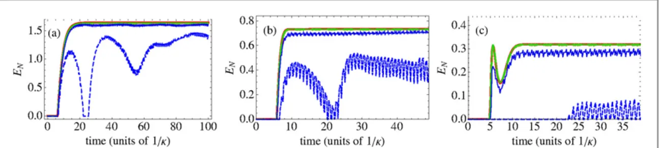
In appendixBwe describe the derivation of the effective linearized equations that we have studied in the preceding sections and that is based on the elimination of fast rotating terms and on the expansion of the linearized coupling strength at lowest order in gj. Here we analyze the limit of validity of these approximations by solving numerically the system dynamics with the inclusion of the non-resonant terms expanded at different orders in powers of gj. Infigures5and6the red lines are evaluated without the non-resonant terms(i.e., the treatment of the preceding sections), while the green and the blue ones take into account the full dynamics. In particular the green lines are computed by expanding the averagefields α(t) and βj(t) (that have been introduced in equation(2) and discussed in appendixB), at the lowest relevant order in powers of g, while for the blue ones
they have been expanded at sixth order in powers of g. Moreover, the green line results are found considering only the steady state solution forα(t) and βj(t), while the blue lines are computed taking into account their full dynamics(that includes also the transient regime before the steady state is reached) with initial condition α (0) = βj(0) = 0.
Infigure5we compare the time evolution of the entanglement evaluated with and without the time-dependent terms when G2> G1. The parameters used in these plots are consistent with those used infigure2. Specifically the three red curves in figures5(a), (b) and (c), that are barely visible because almost entirely covered
by the green curves, are equal to the three lowest curves infigure2. We observe that the green and the red lines are always very close, meaning that the linearized RWA treatment is a very good approximation of the full dynamics whenα(t) and βj(t) can be expanded at lowest order in g. Nevertheless, we note that if the mechanical
Figure 5. Comparison of the time evolution of ENevaluated with and without the non-resonant terms, when G2> G1. The red lines
are evaluated with the model described by equations(4)–(6) that does not take into account the non-resonant terms The green lines are evaluated with equation(B.23), which takes into account the non-resonant terms by considering the expansion of the steady state solutions ofα(t) and βj(t), at first order in g as defined in equation (B.22). The blue lines are evaluated instead with equation (B.19) by
considering the expansion forα(t) and βj(t), calculated iteratively with equations (B.6), (B.9)–(B.12), up to sixth order in g; in
particular these results take into account the full dynamics of the averagefields α(t) and βj(t), with initial condition α(0) = βj(0) = 0,
and not only the steady state as in the case of the green lines. The solid lines refer toω2= 100κ and ω1= 50κ, while the dashed lines
refer toω2= 50κ and ω1= 25κ. The other parameters are G2= κ, Δ = 0.01κ, γ = 10−4κ, and g = 10−4κ. Moreover in (a)
G1=0.918 ,k n¯1=200,n¯2=100;in(b) G1=0.82 ,k n¯1=1000,n¯2=500;in(c) G1=0.75 ,k n¯1=2000,n¯2=1000.
Figure 6. Comparison of the time evolution of ENevaluated with and without the non-resonant terms, when G1= G2. The insets
report the corresponding average photon number d da a .ˆ† ˆ Red, green and blue lines are evaluated as infigure5. The solid lines are
found forΔ = 0.01κ and the dashed lines for Δ = 5κ. In (a)g=0.03 ,k w1=58 ,k w2=100 ,k n¯1= and n2 ¯ =2 1;in(b)
n 0.01 , 1 58 , 2 100 , ¯1 2
g= k w = k w = k = and n¯ =2 1;in(c)g=0.001 ,k w1=51 ,k w2=100 ,k n¯1=20andn¯ =2 10.The other
frequencies are not large enough and higher order terms are taken into account together with the full dynamics ofα(t) and βj(t), then the results can be significantly different as described by the blue curves. Specifically, the solid-blue lines are evaluated for sufficiently large values of the mechanical frequencies so that the condition in equation(3) is well fulfilled, and the effective linearized RWA dynamics recovers with significant accuracy the
one determined with the inclusion of the non-resonant terms The dashed-blue lines are instead evaluated for smaller frequencies. In this case it is evident that the non-resonant terms have a significant role in the system dynamics and that the lowest order expansion of the coefficients α(t) and βj(t) does not provide an accurate description. We note that according to equation(3), in order to eliminate the fast rotating terms, the ratios ωj/Gj have to be much larger than one. Although the dashed-blue curves are evaluated for a ratioω1/G1of roughly 25, which can be considered significantly large, we have found, indeed, that it is not enough for a faithful
approximation of the system dynamics with the model discussed in the preceding sections. The conclusive analysis of these cases would, possibly, require a non-perturbative approach that is beyond the scope of the present work. Afinal remark is in order. We have verified that the discrepancy between the dashed-blue lines and the red ones is due to the combined effect of the higher order terms and of the transient initial dynamics ofα(t) andβj(t). Specifically, when we consider either the lowest order terms and the transient dynamics, or the higher order terms and only the steady state ofα(t) and βj(t), the corresponding results for the entanglement dynamics are very similar to the red lines.
Infigure6we study the case of equal couplings G1= G2. In this case solid and dashed lines differ in the values of the cavity detuningΔ. In general larger Δ (dashed lines) corresponds to smaller entanglement, and the results evaluated by including the counter-rotating terms tends to exhibit larger entanglement than the corresponding ones obtained without the non-resonant terms. The solid curves are found with smallerΔ. In this case red, green and blue lines are very close when the mechanical dissipation is sufficiently large as in figure6(a). Larger
discrepancies are found when the mechanical dissipation is reduced as infigures6(b) and (c), especially at
relatively large time. We observe in fact that, while the red curves for the entanglement decay to zero at large time, the corresponding green and blue lines seem to approach afinite sizable value. As shown by the insets, when this different behavior is observed, the average photon number in the cavity tends to diverge. This is a signature of the fact that the full dynamics including counter-rotating terms is actually unstable, even though the RWA dynamics without these terms is stable(see equation (9)). We have confirmed the unstable nature of the
time-dependent dynamics by calculating the Floquet exponents of the dynamical equations of the system. In fact, whenα(t) and βj(t) are considered in their steady state, one has a system of linear differential equations with periodic, time-dependent coefficients (see appendixB), and the Floquet theory can be applied in this case [52];
we have verified that for the parameters of figure6there is always at least one positive Floquet exponent, meaning that the system is unstable. This implies that, in general, the corresponding results are well-grounded only for relatively short time until the populations are not exceedingly large. On the other hand, our results show that in a pulsed experiment with the parameters offigure6, these instabilities do not constitute a serious
hindrance to the creation of significant entanglement at finite times.
Therefore, when the mechanical frequencies are sufficiently large (wj 102k) (and, limited only to the case of equal couplings, when also mechanical damping is not too small), the effective linearized RWA dynamics obtained by neglecting the counter-rotating terms approximates with very good accuracy the full system dynamics.
6. Strategies for the experimental detection of mechanical entanglement
Wefinally discuss how to detect the generated mechanical entanglement between the two MRs at different frequencies. The present entanglement describes EPR-like correlations between the quadratures of the two MRs and therefore we need to perform homodyne-like detection of these quadratures. In the linearized regime we are considering the state of the two MRs is a Gaussian CV state, which is fully characterized by the matrix of all second-order correlations between the mechanical quadratures. Therefore from the measurement of these correlations one can extract the logarithmic negativity EN. One does not typically have direct access to the mechanical quadratures, but one can exploit the currently available possibility to perform low-noise and highly efficient homodyne detection of optical and microwave fields, and implement an efficient transfer of the mechanical phase-space quadratures onto the optical/microwave field.
As suggested in[53] and then implemented in the electromechanical entanglement experiment of [5], the
motional quadratures of a MR can be read by homodyning the output of an additional‘probe’ cavity mode. In particular, if the readout cavity mode is driven by a much weaker laser so that its back-action on the mechanical mode can be neglected, and resonant with thefirst red sideband of the mode, i.e., with a detuning
j , 1, 2, j p j w
D = = the probe mode adiabatically follows the MR dynamics, and the output of the readout cavity ajoutis given by(see figure1) [53]
aj iG b a , j 1, 2, 46 j p j j out in ( ) kd = + =
withGjpthe very small optomechanical coupling with the probe mode. Therefore using a probe mode for each MR, changing the phases of the corresponding local oscillator, and measuring the correlations between the probe mode outputs, one can then detect all the entries of the correlation matrix and from them numerically extract the logarithmic negativity EN.
6.1. Concluding remarks
We have studied in detail a general scheme for the generation of large and robust CV entanglement between two MRs with different frequencies through their coupling with a single, bichromatically driven cavity mode. The scheme extends and generalizes in various directions similar schemes exploiting driven cavity modes
[34,36,38,44] for entangling two MRs or two cavity modes. The scheme is able to generate a remarkably large
entanglement between two macroscopic oscillators in the stationary state, i.e., with virtually infinite lifetime, and it is quite robust because one can achieve appreciably large CV entanglement even with thermal occupancies of the order of 103. The scheme is particularly efficient in the limit where counter-rotating terms due to the bichromatic driving of the cavity mode are negligible, and we have verified with a careful numerical analysis that this is well justified when the two mechanical frequencies are sufficiently largewj 102k.
Acknowledgments
This work has been supported by the European Commission(ITN-Marie Curie project cQOM, Grant No. 290161, and FET-Open Project iQUOEMS, Grant No. 323924), by MIUR (PRIN 2011).
Appendix A. Normal modes and Hamiltonian dynamics
It is straightforward to see that the diagonal form of the interaction Hamiltonian of equation(10) is
Hˆeff 0 1ˆ ˆ1 1 1ˆ ˆ1 2ˆ ˆ2 2, (A.1) † † † l b b l a a l a a = + + where a
cos sin , A.2
1 2
ˆ ˆ ˆ ( )
a = qb + qd
a
cos sin , A.3
2 2
ˆ ˆ ˆ ( )
a = qd - qb
define the other two normal modes together with the dark mode ,b introduced in equationˆ1 (11), with θ defined
by the condition tan 2q = -2 D while the eigenvalues are given by, l0=0l1= (D - D˜ ) l2 2=
2,
(D + D˜ ) withD = D +˜ 2 42.
The normal modes allows to understand the dynamics in the absence of optical and mechanical damping processes. In fact, from equation(A.1) one can easily derive the Heisenberg evolution of the mechanical bosonic
operators. By inverting equations(11), (12) one has, b tˆ ( )1 coshrˆ ( )1 t sinhrˆ ( ) ˆ ( )2 t b t2 †
d = b - b d =
r t r t
cosh ˆ ( )2 sinh ˆ ( )1 †
b - b and usingaj( )t =eiltaj( )0 ,j = 1, 2,andβ1(t) = β1(0), one gets
b t r
r t t t
r t t a
cosh 0
sinh exp i
2 cos 2 i cos 2 sin 2 0
i sinh sin 2 exp i
2 sin 2 0 A.4 1 1 2 ˆ ( ) ˆ ( ) ˜ ˜ ˆ ( ) ˜ ˆ ( ) ( ) † ⎡ ⎣⎢ ⎤ ⎦⎥ ⎡ ⎣ ⎢ ⎤ ⎦ ⎥ ⎡ ⎣⎢ ⎤ ⎦⎥ d b q b q d = - D D - D - D D b t r r t t t r t t a sinh 0 cosh exp i
2 cos 2 i cos 2 sin 2 0
i cosh sin 2 exp i
2 sin 2 0 . A.5 2 1 2 ˆ ( ) ˆ ( ) ˜ ˜ ˆ ( ) ˜ ˆ ( ) ( ) † ⎡ ⎣⎢ ⎤ ⎦⎥ ⎡ ⎣ ⎢ ⎤ ⎦ ⎥ ⎡ ⎣⎢ ⎤ ⎦⎥ d b q b q d = -+ - D D + D + -D D
We now look for special time instants at which the two mechanical modes can be strongly entangled. A necessary condition for such dynamical entanglement is that at these times, the cavity mode must be decoupled from the mechanical modes and equations(A.4), (A.5) show that it occurs whensinD˜t 2=0,i.e.,
b t r r b
r r b
cosh e sinh 0
sinh cosh 1 e 0 , A.6
p 1 2 i 2 1 i 2 p p
( )
(
)
ˆ ˆ ( ) ˆ ( )† ( ) ⎡⎣ ⎤⎦ d d d = -+ -f f b t r r b r r b e cosh sinh 0sinh cosh 1 e 0 , A.7
p 2 i 2 2 2 i 1 p p
( )
(
)
ˆ ˆ ( ) ˆ ( ) ( ) † † ⎡⎣ ⎤⎦ d d d = -- -f f wherefp=pp 1( + D D In particular, if e˜). ifp = -1one getsb tˆ1
( )
p cosh 2r bˆ ( )1 0 sinh 2r bˆ ( )2 0 , (A.8)†
d = d + d
bˆ2
( )
tp cosh 2r bˆ ( )2 0 sinh 2r bˆ ( )1 0 , (A.9)† †
d = - d - d
i.e., the state of the two MRs at time tpis the result of the application of the two-mode squeezing operator with squeezing parameter r S2 , ˆ ( )2r (see equation (14)) to their initial state. In the usual case of an initial thermal state
for the two MRs with mean thermal phonon numbersn ,¯j the state at time tpis therefore a two-mode squeezed thermal state[50] (see equation (32)), with logarithmic negativity [47,48]
E t n n r
n r n n r
1
2 ln 1 cosh 8
1 sinh 8 4 1 cosh 4 , A.10
N p 2 2 4 2 2 2 2
( )
(
)
(
)
(
)
¯ ¯ ¯ ¯ ¯ ( ) ⎡ ⎣⎢ ⎤ ⎦⎥ = - + + - + + + - + + - +where n¯=n¯1n .¯2 For the relevant case of not too small values of the squeezing parameter r,ENcan be well approximated with its value at equal mean thermal phonon number n¯ =- 0,
EN
( )
tp 4r-ln⎡⎣n¯++1 ,⎤⎦ (A.11) showing that at this interaction time, the entanglement between the MR can be very large, even if starting from a relatively hot state, by properly tuning the ratio G2/G1, i.e., the intensity of the two tones. This large mechanical entanglement is achieved when the condition eifp= -1is also satisfied for a given integer p. This is obtained for any odd p whenΔ = 0, or by properly adjusting the value offor a givenD ¹0,i.e., ifd p d p d d d p d p 2 4 odd, 0 2 , . A.12 p 2 2 2 ( ) ( ) ( ) = D -- < < ¹
This dynamical scheme for the generation of CV mechanical entanglement is similar to the Bogoliubov scheme proposed in[45] for entangling two optical cavity modes. It is extremely hard however to use it for entangling
two mechanical modes as in the present case, because the cavity decay rate is comparable toandΔ in typical situations, thereby strongly affecting the ideal Hamiltonian dynamics described here.
Appendix B. Linearization of the optomechanical dynamics with two-frequency drives
The system dynamics is described by the following QLEa a E E a g b b g b b a b b g a a b j i i e e 2 i , 2 i i 1, 2, B.1 t t j j j j j j j 0 1 i 2 i in 1 1 1 2 2 2 in
(
)
(
)
(
)
ˆ˙ ˆ ˆ ˆ ˆ ˆ ˆ ˆ ˆ˙ ˆ ˆ ˆ ˆ ( ) † † † ⎜ ⎟ ⎡ ⎣ ⎤⎦ ⎡⎣ ⎤⎦ ⎡ ⎣⎢ ⎤⎦⎥ ⎛ ⎝ ⎞⎠ k w k g w g = - + D + - + + - + + + = - + - + = w w - - + +where, here, differently from the description used in section2, we are representing the cavityfield in a reference frame rotating at the frequencyω0− (ω2− ω1)/2, and we have introduced the frequencies
2 .
2 1
w= w w The other parameters and operators are defined in the main text.
If we perform a time dependent displacement, for both cavity and mechanical degrees of freedom, of the form a t a t t b t b t t , , B.2 j j j ˆ ( ) ˆ ( ) ( ) ˆ ( ) ˆ ( ) ( ) ( ) d a d b = + = +
the QLE reduce to the form a g t g t a A t a t g b b g b b g b b g b b a i 2i Re 2i Re i 2 i i , B.3 0 1 1 2 2 in 1 1 1 2 2 2 1 1 1 2 2 2
(
)
(
)
(
)
(
)
{
(
)
}
ˆ ˙ ( ) ( ) ˆ ( ) ˆ ( ) ˆ ˆ ˆ ˆ ˆ ˆ ˆ ˆ ˆ ( ) † † † † ⎡⎣ ⎤⎦ ⎡⎣ ⎤⎦ ⎡ ⎣⎢ ⎤⎦⎥ ⎡ ⎣⎢ ⎤⎦⎥ d k w b b d k a d d d d d d d d d = - + D + + + - + - + + + - + + + -b b B t b g t a t a g a a 2 i i i i , B.4 j j j j j j j j j in ˆ ˙ ˆ ( ) ˆ ( ) ˆ† ( ) ˆ ˆ† ˆ ( ) ⎜ ⎟ ⎛ ⎝ ⎞⎠ ⎡⎣ * ⎤⎦ d g w d g a d a d d d = - + - + - +-where the new driving terms, A(t) and Bj(t) read
A t E E t t t g t g t t B t t t t g t i e e i 2i Re Re , 2 i i . B.5 t t j j j j j j 1 i 2 i 0 1 1 2 2 2
(
)
(
)
( ) ( ) ( ) ( ) ( ) ( ) ( ) ( ) ⎜ ⎟ ( ) ∣ ( )∣ ( ) ⎡⎣ ⎤⎦ ⎡ ⎣ ⎤⎦ ⎡⎣ ⎤⎦ ⎡⎣ ⎤⎦ ⎛ ⎝ ⎞⎠ a k w a b b a b g w b a = - + - ¶ ¶ - + D + - + = - ¶ ¶ - + -w w -+ +When g1and g2are sufficiently small and we chose α(t) and βj(t) such that A(t) = 0 and Bj(t) = 0, then the nonlinear terms, i.e. the last terms in the two equations(B.3) and (B.4), can be neglected. The equations A(t) = 0
and Bj(t) = 0 define a set of nonlinear differential equations with periodic driving for the parameters α(t) and βj(t). The solution can be evaluated perturbatively in the small parameters g1and g2[46]. Here we assume g1= g2≡ g and we observe that the solutions for α(t) and βj(t), with initial condition α(0) = βj(0) = 0, contain, respectively, only even and odd powers of g,
t g t t g t , . B.6 p p p p j p p p j p 0 even 1 odd ( ) ( ) ( ) ( ) ( ) ( ) ( )
å
å
a a b b = = = ¥ = ¥The equations for each component of these expansions can be written in the form
t z t t t w t t , , B.7 p p p j p j jp p ˙ ( ) ( ) ( ) ˙ ( ) ( ) ( ) ( ) ( ) ( ) ( ) ( ) ( ) ( ) a a b b = - + X = - + X a b where z w i , 2 i , B.8 j j j 0
(
)
( ) k w g w = + D + = +-and the driving terms are defined recursively as
t t t t t t t 2i Re Re , i , B.9 p q p q p q p q p q p q p q 0 1 1 1 2 1 0 1 1
(
)
( ) ( ) ( ) ( ) ( ) ( ) ( ) ( ) ( ) ( ) ( ) ( ) ( ) ( ) ( ) ⎡⎣ ⎤⎦ ⎡⎣ ⎤⎦ *å
å
a b b a a X = -´ + X = -a b = -- -- -=-with the initial condition
t E E t e e , 0. B.10 t t 0 1 i 2 i 0 ( ) ( ) ( ) ( ) ( ) X = + X = a w w b - + +
In particular they can always be rewritten as sums of exponential functions of the form t t e , e , B.11 p n p n t p n p n t , , p n p n , , ( ) ( ) ( ) ( ) ( ) ( ) ( ) ( ) ( )
å
å
c c X = X = a a z b b z a b withc(p n, )c(p n, ) (zp n, )a b a andz(bp n, )time-independent complex coefficients, whose specific form can be computed iteratively. Moreover, the expression fora( )p( )t and t
j p
( )
( )
b are found integrating equation(B.7) and are given by
t z t w e e , e e . B.12 p n p n p n t zt j p n p n j p n t w t , , , , p n p n j , ,
(
)
(
)
( ) ( ) ( ) ( ) ( ) ( ) ( ) ( ) ( ) ( ) ( )å
å
a c z b c z = + -= + -a a z b b z -a bWe note that all the coefficientsz(p n, )
a andz(bp n,)have non-positive real parts, Re[z(ap n, )], Re[z(bp n, )]0,thus the
large-time solutions p t p t
st
( ) ( )
( ) ( )
a ¥ ºa andb( )jp(t ¥ º) b( )jp,st( )t are found from equation(B.12) by
keeping only the terms for whichz(ap n,)andz(p n,)
b are purely imaginary, that can be shown to be equal to ni w+ with n odd and even integer respectively. In particularast( )p( )t andb˜j( ),stp( )t are periodic functions(with period 2π/ω+) which contains frequency components that are, respectively, odd and even multiples of ω+,
t z n t w n i e , i e , B.13 p n p n p p n n t j p n p n p p n j n t st 1 odd 1 , i ,st 1 even 1 , i ( ) ˜ ( ) ˜ ( ) ( ) ( ) ( ) ( )
å
å
a c w b c w = + = + a w b w = -+ + = -+ + + +where z and wjare defined in equation (B.8), andc˜a(p n,)( )t andc˜b(p n, )( )t are the coefficients that correspond to those particular parametersz(ap n,)andz(p n, )
b that are imaginary. B.1. Resonant and non-resonant terms
The QLE, in the interaction picture with respect to the Hamiltonian Hˆ0 ( a a† 1 1b bˆ ˆ1 2 2b b ,ˆ ˆ )2
† † w w w = - + + reduce to a a a g t g t a t g b b g b b b b b g t a i 2 2i Re Re i e e e e e , 2 i e e h.c. . B.14 t t t t t j j j j j j t t 0 in 1 1 2 2 i 1 1 i 1 i 2 2 i 2 i in i i j 1 1 2 2
(
)
(
)
(
)
(
)
ˆ ˙ ˆ ˆ ( ) ( ) ˆ ( ) ˆ ˆ ˆ ˆ ˆ ˙ ˆ ˆ ( ) ˆ ( ) † † † ⎡⎣ ⎤⎦ ⎡⎣ ⎤⎦ ⎡ ⎣⎢ ⎤ ⎦⎥ ⎡⎣ ⎤⎦ d k d k b b d a d d d d d gd g a d = - + D + + + - + + + = - + - + w w w w w w w-Before proceeding, we note that we can include the dc component ofβj(t) into the cavity detuning, hence we
introduce 2 j gjRe pgp , w 0 1,2 p j ,0 [ ˜ ] ( )
å
D = D + = å cbaccording to the notation introduced in equation(8),
g w . B.15 p p p j j ,0 dc ˜ ( ) ( )
å
cb ºbMoreover we can isolate the resonant terms of the QLE, namely the terms with time-independent coefficients, by considering the lowest order frequency components ofα(t), i.e.
g z i , B.16 p p p, 1 ˜ ( ) ( )
å
a c w = a +corresponding to the frequencies±ω+, and defining
t t t t , e , B.17 j j j t dc i ¯ ( ) ( ) ¯ ( ) ( ) ( ) b b b a a a = -= - w + + +
t t e i t . B.18 ¯ ( ) ( ) ( ) a =a - w a - - + -Thereby wefind a a g b g b a F t b b g a b F t b b g a b F t i i i 2 , 2 i , 2 i , B.19 a b b 1 1 2 2 in 1 1 1 1 1 1 in 2 2 2 2 2 2 in 1 2 ˆ ˙ ( ) ˆ ˆ ˆ ˆ ( ) ˆ ˙ ˆ ˆ ˆ ( ) ˆ ˙ ˆ ˆ ˆ ( ) ( ) † † * d k d a d a d k d g d a d g d g d a d g = - + D - -+ + = - - + + = - - + + - + -+
where F ta( ),Fb1( )t andFb2( )t account for the terms with time-dependent coefficients and are given by
F t g t g t a t g b g b t g b t g b F t g t a t a F t g t a t a 2i Re Re i e e e i e e i e e , i e e e , i e e e . B.20 a t t t t t t t b t t t b t t t 1 1 2 2 i 1 1 i 2 2 i i 1 1 i i 2 2 i 1 i i i 2 i i i 1 2 1 2 1 1 2 2
(
)
(
)
( ) ¯ ( ) ¯ ( ) ˆ ( ) ˆ ˆ ¯ ( ) ˆ ¯ ( ) ˆ ( ) ¯ ( ) ˆ ( ) ˆ ( ) ( ) ˆ ¯ ( ) ˆ ( ) † † † † ⎡⎣ ⎤⎦ ⎡⎣ ⎤⎦ ⎡⎣ ⎤⎦ ⎡⎣ ⎤⎦ * * b b d a d d a d a d a d a d a d a d = + + - + - -= - + = - + w w w w w w w w w w w w w -- + -- -+ -- -- ---In particular we can introduce the linearized coupling strength G1(tot)=ga-and G2tot g , ( )= a
+ withα±defined in equation(B.16). The expressions introduced in equation (7) correspond to the expansion of these parameters
at zeroth order in g(see also equation (B.22)).
We are interested in the regime in which the terms in equations(B.20) with time-dependent coefficients are
negligible. They can be neglected when gj∣ast( )∣t ,gj∣ ¯bj,st( )∣t ,kmin{w w1, 2,∣w1-w2∣}.In particular this condition is true when it is valid for the lowest order term in the expansion in power of g. In details, the non resonant terms can be neglected when
g a ,kmin
{
w w1, 2, w1-w2}
. (B.21) When this condition is fulfilled the parameters α(t) and βj(t) can be safely expanded at the lowest order in g. Specifically they can be approximated asE z E z t t g w t g t g w w i i , i i , e e , i , i 2i e 2i e . B.22 t t j j j j j j j j j t j t 1 2 st st0 i i dc ,st 1,st dc 2i 2i ( ) ( ) ¯ ( ) ( ) ( ) ( ) ( ) ⎡⎣ ⎤⎦ ⎡ ⎣ ⎢ ⎤ ⎦ ⎥ * * * * a w a w a a a a b a a a a b b b a a w a a w -+ = + -+ = -- + w w w w -+ + + - - + - - + + - + + - + -+ + + + +
Moreover the parametersa¯ ( )t defined in equation (B.18) are zero. Using these expressions the QLE in equation(B.19) can be rewritten as
a a G b G b a F t b b G a b F t b b G a b F t i i i 2 , 2 i , 2 i , B.23 a b b 1 1 2 2 in 1 1 1 1 1 1 in 2 2 2 2 2 2 in 1 2 ˆ ˙ ( ) ˆ ˆ ˆ ˆ ( ) ˆ ˙ ˆ ˆ ˆ ( ) ˆ ˙ ˆ ˆ ˆ ( ) ( ) † † * d k d d d k d g d d g d g d d g = - + D - -+ + = - - + + = - - + +
with G1and G2defined in equation (7) and
F t g t g t a t g b g b 2i Re Re ie e e , a t t t 1 2 1,st 1 2 2 2,st 1 i st0