Power quality in power drive systems

D

M

I

E

P

M

I

E

XXVI

C

Phd Candidate:

A

N

Thesis Title:

P

OWER

Q

UALITY IN

P

OWER

D

RIVE

S

YSTEMS

Supervisor:

P

.

A

D

N

Coordinator:

2

I

I

... 10

1.

P

Q

... 15

1.1 Power Quality definition ... 15

1.2 Power quality progression ... 16

1.3 Power Quality terminology... 18

1.4 Power Quality Issues ... 24

1.5 Role of Power Electronics in Improving Quality of AC Grid Power ... 27

1.5.1 Flexible AC Transmission Systems (FACTS) Operating Principle ... 28

1.5.2 Shunt-Connected Controllers ... 29

1.5.3 Series-Connected Controllers... 30

2.

U

... 33

2.1 Introduction ... 34

2.1.1 Ultracapacitors construction ... 35

2.1.2 Typical Applications ... 36

2.2 The Gantry Crane System... 39

2.3 The Ultracapacitors Storage System ... 39

2.4 Gantry Crane System ... 41

2.5 Electrical system layout ... 47

2.6 Ultracapacitors model ... 50

2.7 Ultracapacitors Sizing ... 52

2.7 System modeling ... 55

2.8 Power Flow regulation strategy ... 59

2.8.1 K parameter definition ... 59

2.8.2 H and H1 definition ... 60

2.8.3 H1 and K regulation ... 60

2.9 Gantry crane model wilth UC storage ... 62

2.10 Experimental validation of the model ... 64

2.12.1 Light load cycle ... 68

2.12.2 Heavy load cycle ... 72

3

2.14 Economic Evaluation of the simulation results... 92

2.14.1 Cost of Investment... 93

2.14.2 Cost of the electric energy ... 95

2.14.3 Payback period ... 96

3.

A

F

-E

C

... 99

3.1 Introduction ... 99

3.2 Active Front End operating principle ... 101

3.3 Key Features of Active Front-End Inverters ... 106

3.3.1 Comparison between Traditional Drives and Active Front-End Drives ... 108

3.4 System configuration... 111

3.5 Compensation Characteristics of an Active Drive ... 112

3.6 Steady-State Control ... 113

3.7 The d-q theory ... 116

3.8 Deriving the d-q model... 122

3.9 Selecting the Rotating Coordinate System ... 125

3.10 Power Definitions in d-q Coordinate System ... 128

3.11 Dynamic Equations for an Active Front-End Converter ... 131

3.12 Control of the Active Drive ... 133

3.12.1 Feed-Back Control ... 134

3.12.2 Estimating Angular Frequency of Source Voltages ... 136

3.12.3 Input-Output Linearization Control ... 137

3.12.4 Feed-Forward Compensation ... 139

3.12.5 Complete Control Scheme for Active Front-End Converter ... 141

3.13 Simulation Model ... 143

3.14 Simulation Results ... 145

3.14.1 Normal Condition mode ... 145

3.14.2 AFE in presence of voltge sags ... 149

3.14.2.1 Single phase voltage sag ... 151

3.14.2.2 Double phase voltage Sags ... 154

3.14.3 AFE in presence of voltge notches ... 156

3.14.3.1 Single phase voltage notches ... 158

3.14.3.2 Double phase voltage notches ... 162

4

5.

A

II

–

EMC

M

... 176

5.1 Introduction ... 176

5.2 Apparatus Conformity Assestement... 177

5.3 EMC Testing ... 179 5.4 Test Set-Up ... 180 5.5 Experimental results ... 183

C

... 189

R

... 191

P

... 196

5

List of Figures

Fig. 1.1: Crest factor for sinusoidal waves ... 19

Fig. 1.2: Distorted waveform ... 20

Fig. 1.3: Power Quality issues... 25

Fig. 2.1: Ultracapacitor charge separation ... 36

Fig. 2.2: Bridge crane operation ... 39

Fig. 2.3: Absorbed/Delivered power of the lifting motor ... 40

Fig. 2.4: Circuit diagram of the bridge crane drive with recovery capabilities ... 40

Fig. 2.5: Geometry of the system ... 42

Fig. 2.6: Load speed, trajectory and Acceleration during the lifting/descending process. .... 43

Fig. 2.7: Lifting/descending motor torque, energy, power during the lifting/descending process ... 43

Fig. 2.8: Load speed, trajectory and Acceleration during the rotation process. ... 44

Fig. 2.9: Rotation motor torque, energy, power during the rotation process. ... 45

Fig. 2.10: Load speed, trajectory and Acceleration during the translation process. ... 45

Fig. 2.11: Translation motor torque, energy, power during the translation process. ... 46

Fig. 2.12: Load speed, trajectory and Acceleration during the scroll process... 46

Fig. 2.13: Scroll motor torque, energy, power during the scroll process. ... 47

Fig. 2.14: Blocks scheme of the electrical drive ... 48

Fig. 2.15: Bidirectional dc-dc converter for UCs management ... 48

Fig. 2.16: Simplified model of the ultracapacitors ... 51

Fig. 2.17: Wiring diagram of the ultracapacitors ... 54

Fig. 2.18: Load lifting – UCs discharge... 56

Fig. 2.19: Load descending – UCs recharge ... 56

Fig. 2.20: Implemented simulation model ... 57

Fig. 2.21: Drive simulation model... 58

Fig. 2.22: Regulation strategy flow chart ... 62

Fig. 2.23: Drive diagram ... 63

Fig. 2.24: Lifting prototype of Ultracapacitors Storage system ... 65

Fig. 2.25: Motor speed and torque in function of time ... 67

Fig. 2.26: Motor drive power in function of time... 68

Fig. 2.27: Light load cycle measured voltages vs time ... 68

Fig. 2.28: Light load cycle measured currents vs time ... 69

Fig. 2.29: Light load cycle measured motor power demand vs time ... 69

Fig. 2.30: Light load cycle SIMULATED motor power demand vs time ... 70

Fig. 2.31: Light load cycle SIMULATED speed vs time ... 70

Fig. 2.32: Light load cycle SIMULATED torque vs time ... 70

Fig. 2.33: Light load cycle SIMULATED voltages vs time ... 71

Fig. 2.34: Light load cycle SIMULATED currents vs time ... 71

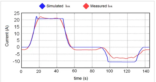
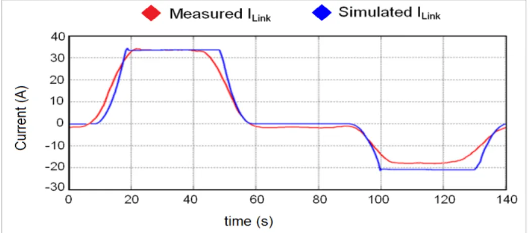
Fig. 2.35: Light load cycle – comparison between simulated and measured Ilink ... 72

Fig. 2.36: Heavy load cycle measured voltages vs time ... 72

Fig. 2.37: Heavy load cycle measured currents vs time ... 73

6

Fig. 2.39: Heavy load cycle SIMULATED motor power demand vs time ... 74

Fig. 2.40: Heavy load cycle SIMULATED torque vs time ... 74

Fig. 2.41: Heavy load cycle SIMULATED voltages vs time... 75

Fig. 2.42: Heavy load cycle SIMULATED currents vs time ... 75

Fig. 2.43: Heavy load cycle – comparison between simulated and measured Ilink ... 75

Fig. 2.44: DC-link Voltage vs time for K = 0, C = 63F, H = 0; H1 = 1. ... 77

Fig. 2.45: Traction motor simulated power demanded vs time for K = 0, C = 63F, H = 0; H1 = 1. ... 77

Fig. 2.46: Grid current Igid vs time for K = 0, C = 63F, H = 0; H1 = 1. ... 78

Fig. 2.47: Traction motor shaft speed vs time for K = 0, C = 63F, H = 0; H1 = 1. ... 78

Fig. 2.48: Motor Reference and current Torque vs time for K = 0, C = 63F, H=0; H1=1. .... 79

Fig. 2.49: Energy flow for K = 0, C = 63F, H=0; H1=1 ... 79

Fig. 2.50: Simulated voltages for K=0, C=63F, H=0.6, H1=1.3. ... 80

Fig. 2.51: Simulated currents for K=0, C=63F, H=0.6, H1=1.3. ... 80

Fig. 2.52: Simulated voltages for K=0.5, C=63F, H=0.6, H1=1.3. ... 81

Fig. 2.53: Simulated currents for K=0.5, C=63F, H=0.6, H1=1.3. ... 81

Fig. 2.54: Simulated voltages for K=1, C=63F, H=0.8, H1=1.3. ... 82

Fig. 2.55: Simulated currents for K=1, C=63F, H=0.8, H1=1.3. ... 82

Fig. 2.56: Simulated voltages for K=1, C=75.78F, H=0.8, H1=1.3. ... 83

Fig. 2.57: Simulated currents for K=1, C=75.78F, H=0.8, H1=1.3. ... 84

Fig. 2.58: Simulated power grid for K=0, C=63F, H=0, H1=1 ... 85

Fig. 2.59: Simulated energy grid for K=0, C=63F, H=0, H1=1 ... 85

Fig. 2.60: Simulated power grid for K=0, C=63F, H=0.6, H1=1 ... 86

Fig. 2.61: Simulated energy grid for K=0, C=63F, H=0.6, H1=1 ... 86

Fig. 2.62: Simulated power grid for K=0.5, C=63F, H=0.6, H1=1.3 ... 87

Fig. 2.63: Simulated energy grid for K=0.5, C=63F, H=0.6, H1=1.3 ... 87

Fig. 2.64: Simulated power grid for K=1, C=63F, H=0.8, H1=1.3 ... 88

Fig. 2.65: Simulated energy grid for K=1, C=63F, H=0.8, H1=1.3 ... 88

Fig. 2.66: Simulated power grid for K=1, C=75.78F, H=0.8, H1=1.3 ... 89

Fig. 2.67: Simulated energy grid for K=1, C=75.78F, H=0.8, H1=1.3 ... 89

Fig. 2.68: Delta T vs I for duty cycle = 50%... 91

Fig. 2.69: Specific Cost/Wh for different types of cells and voltages. ... 94

Fig. 2.70: Payback period – Case 2 ... 97

Fig. 2.71: Payback period – Case 3 ... 97

Fig. 2.72: Payback period – Case 4 ... 98

Fig. 2.73: Payback period – Case 5 ... 98

Fig. 3.1: Active front-end induction motor drive system ... 102

Fig. 3.2: Per-phase equivalent circuit ... 103

Fig. 3.3: PF=1 during motor mode ... 104

Fig. 3.4: PF=1 during regenerative mode ... 104

Fig. 3.5: Leading PF during motor mode ... 105

Fig. 3.6: Distributed energy source and utility interface ... 108

Fig. 3.7: Comparison between phase-controlled and active front-end rectifiers ... 109

7

Fig. 3.9: A voltage source rectifier ... 114

Fig. 3.10: Steady-state control of PWM rectifier ... 115

Fig. 3.11: Balanced, 3-phase, Y-connected system ... 117

Fig. 3.12: 3-phase system superponed to a 2-phase d-q system ... 117

Fig. 3.13: Three-phase to two-phase transformation ... 120

Fig. 3.14: Stationary to rotary reference frame, Park’s transformation ... 120

Fig. 3.15: Circuit representation of system mathematical model ... 122

Fig. 3.16: Tracking θe ... 126

Fig. 3.17: DC-link dynamics controlled by line-side converter ... 132

Fig. 3.18: AC-side per-phase equivalent circuit ... 132

Fig. 3.19: DC-side equivalent circuit of an active drive ... 132

Fig. 3.20: High-gain feedback controller for line-side converter ... 135

Fig. 3.21: Supply voltage frequency estimation ... 137

Fig. 3.22: Feed-forward compensation for input-output linearization controller ... 140

Fig. 3.23: Complete control scheme for front-end converter ... 141

Fig. 3.24: Simulation model of the AFE ... 144

Fig. 3.25: AFE Normal Mode simulation results ... 146

Fig. 3.26: Grid iqe and ide ... 147

Fig. 3.27: DC-link voltage over time ... 147

Fig. 3.28: Phase displacement between E1 voltage and I1 current of phase 1 ... 148

Fig. 3.29: Phase displacement between E1 and I1 at 0.2s instant load step change ... 149

Fig. 3.30: Parameters simulation at PCC point Voltage Sag in Phase A at t=0.046s ... 152

Fig. 3.31: Phase displacement between voltage and current in Phase A ... 153

Fig. 3.32: Active Power and Reactive Power Flows, single Voltage Sag ... 153

Fig. 3.33: Parameters simulation at PCC point Voltage Sag in Phase A and B at t=0.046s 154 Fig. 3.34: Phase displacement between voltage and current in Phase B ... 155

Fig. 3.35: Active Power and Reactive Power Flows, Double Voltage Sag ... 156

Fig. 3.36: Voltage Notches ... 157

Fig. 3.37: Single phase Notches Parameters simulation at PCC point Voltage notches occurred in Phase A from t=0.046.s to t=0.1262 ... 158

Fig. 3.38: Phase displacement between voltage and current in Phase A Single Phase Notches event. ... 159

Fig. 3.39: Active Power and Reactive Power flows, single phase Voltage Notches event. . 160

Fig. 3.40: Active and Reactive Currents in the rotary reference frame, single phase notches event. ... 161

Fig. 3.41: Parameters simulation at PCC point for voltage notches in Phase A and Phase B at time interval [0.046s 0.1262s]. ... 162

Fig. 3.42: Phase displacement between voltage and current in Phase B. ... 163

Fig. 3.43: Active and Reactive Power , Double phase Voltage Notches Event. ... 164

Fig. 3.44: Active Currents and Reactive Currents in the rotary reference frame. ... 164

Fig. 4.1: Inverter ... 166

Fig. 4.2: inverter feeding an induction motor ... 169

8

Fig. 4.4: Vector representation of the inverter voltages and the corresponding flux

variation in a time interval ∆T. ... 172

Fig. 4.5: Block diagram of DTC ... 174

Fig. 5.1: Conducted emission testing set-up (current probe method) scheme (top view): 1 EMI receiver 2 ground plane, 3 EUT, 4 non-conductive supports, 5 current probe, 6 power lines, 7 LISN, 8 DC power supply. ... 180

Fig. 5.2: Radiated emission testing set-up scheme (top view): 1 EUT, 2 cables, 3 LISN (Line Impedance Stabilization Network), 4 ground plane, 5 non-conductive supports, 6antenna, 7 EMI receiver. ... 181

Fig. 5.3: architetture of the vehicle system ... 181

Fig. 5.4: Electric wheelchair ... 182

Fig. 5.5: Semi-anechoic chamber with ferrite tiles ... 183

Fig. 5.6: Frequency characteristics of ferrite tiles and pyramidal polystyrene ferrite ... 183

Fig. 5.7: Conducted emissions 150kHz-30MHz. No Emi filter ... 184

Fig. 5.8: Conducted emissions 500kHz-5MHz. No Emi filter ... 184

Fig. 5.9: Radiated Emissions, horizontal polarization ... 185

Fig. 5.10: Radiated Emissions, vertical polarization ... 185

Fig. 5.11: EMI filter ... 186

Fig. 5.12: EMI filter Bode plot... 187

Fig. 5.13: Conducted emissions 150kHz-30MHz. No EMI filter... 187

9

List of Tables

Table 1: A summary of FACTS controllers configuratin ... 32

Table 2: Main features of the lifting system ... 42

Table 3: UCs module main characteristics ... 53

Table 4: Simulation Reference Parameters ... 59

Table 5: Test Drive parameters ... 65

Table 6: Simulation parameters for the Light Load cycle ... 69

Table 7: Simulation parameters for the Heavy Load cycle ... 73

Table 8: Simulation cases ... 76

Table 9: Maximum grid power and energy grid per cycle ... 84

Table 10: Ultracapacitors module specifications ... 91

Table 11: MV consumer cost analysis ... 95

Table 13: Summerized costs and saving for the considered 4 cases ... 96

Table 14: Normal Condition mode simulation parameters ... 145

Table 15: Voltage notches simulation parameters... 157

Table 16: Inverter switches configuration ... 167

Table 17: Vectors applied in various sectors depending on the errors ... 173

10

Introduction

The threatened limitations of conventional electrical power sources have focused a great deal of attention on power, its application, monitoring and correction. Power economics now play a critical role in industry as never before. With the high cost of power generation, transmission, and distribution, it is of paramount concern to effectively monitor and control the use of energy.

The electric utility’s primary goal is to meet the power demand of its customers at all times and under all conditions. But as the electrical demand grows in size and complexity, modifications and additions to existing electric power networks have become increasingly expensive. The measuring and monitoring of electric power have become even more critical because of down time associated with equipment breakdown and material failures.

In modern electrical power systems, electricity is produced at generating stations, transmitted through a high voltage network, and finally distributed to consumers. Due to the rapid increase in power demand, electric power systems have developed extensively during the 20th century, resulting in today’s power industry probably being the largest and most complex industry in the world. Electricity is one of the key elements of any economy, industrialized society or country. A modern power system should provide reliable and uninterrupted services to its customers at a rated voltage and frequency within constrained variation limits. If the supply quality suffers a reduction and is outside those constrained limits, sensitive equipment might trip, and any motors connected on the system might stall.

11

The electrical system should not only be able to provide cheap, safe and secure energy to the consumer, but also to compensate for the continually changing load demand. During that process the quality of power could be distorted by faults on the system, or by the switching of heavy loads within the customers facilities. In the early days of power systems, distortion did not impose severe problems towards end-users or utilities. Engineers first raised the issue in the late 1980s when they discovered that the majority of total equipment interruptions were due to power quality disturbances. Highly interconnected transmission and distribution lines have highlighted the previously small issues in power quality due to the wide propagation of power quality disturbances in the system. The reliability of power systems has improved due to the growth of interconnections between utilities. In the modern industrial world, many electronic and electrical control devices are part of automated processes in order to increase energy efficiency and productivity. However, these control devices are characterized by extreme sensitivity in power quality variations, which has led to growing concern over the quality of the power supplied to the customer.

From the end-user point of view, is important not only the quality of power but also the quantity of power used to supply the loads, that is, the quantity of money the user has to pay for the power supply.

Thus, the work of this thesis is the characterization of a power drive system focused on :

• Minimization of Power supplied by the Grid (Ultracapacitors)

• Optimiziation of Power supplied by the Grid ( Active Front End).

12

In the first part of the thesis a general overview of the Power Quality concept is given. Power Quality related phenomena definitions are presented together with the most common Power Quality issues. Moreover, a general overview of the role of power electronic in contrasting these issues is given together with the most used type of controllers for Power Quality improvements.

The second part of the thesis is focused on the downstream of a power drive, that is, from the rectifier to the load, so the minimization of the grid power.

It is presented a gantry crane system coupled with a storage system based on Ultracapacitors. The aim of the storage system is to minimize the usage of the Grid power, thus, to improve, from the economical point of view, the usage of the power drive, especially if the utilization frequency is relevant.

First an overview of the Ultracapacitors tecnology is given together with the ultracapacitors model used to perform the simulation model.

Afterwards, an overview of the power drive system is given together with the assumed work cycle. The phase which is considered as the Ultracapacitors recovery phase (energy recovery) is the descending phase, in which the energy of the ultracapacitors is recovered and then released during the lifting phase.

All the data related to the gantry crane, such as power, torque, energy, load speed, load acceleration and load trajectory are technical real data which are used as input data for the simulation model. So, what was done was to take real data as a reference for the simulation model.

Once the model of the gantry crane coupled with the ultracapacitors storage system is obtained, a procedure of sizing the

13

ultracapacitors based on the energy related to the descending of the load (for the sizing it is considered the maximum of the load = 50 tons).

Aftwards a power flow regulatin strategy control strategy is developed. The aim of this regulation strategy is to have different degrees of freedom in choosing the appropriate ammount of Grid Power, that is, to have balanced or unbalanced grid power flow during the entire process.

Experimental measurements for two different load conditions performed on a scaled experimental set up are presented and used to validate the simulation model. Afterwards simulation results are presented for different regulation strategy parameters.

At the end of the second part an economic evaluation is done in order to investigate the payback time of the investment for different simulation cases.

The third part of the thesis is mainly focused in the upstream of the power drive, that is, the optimization of grid power utilization (second main point of the thesis).

In this part it is presented the simulation model of an Active Front End with Reactive Power compensation capabilities, which provides, too, the Active Power to the own load.

First an overview of the Active Front End concept is given, together with the operating principle. Main keyfeatures of Active Fron End are presented both with a comparison between Active Front Ends drives and traditionals drives.

The AFE is used to compensate the Reactive power in such a way that the Power Factor is unity.

The steady state characteristics as well as differential equations describing the dynamics of the front-end rectifier are shown.

14

The dynamic equations describing the dynamic model of the system are obtained based on the d-q theory. The Control model is obtained and implemented in Matlab-Simulink platform. Feed-forward compensation was used to achieve a better dynamic response.

Different Resistive-inductive loads are connected in the PCC point to simulate the other user of the Grid, which contribute in the pollution of the network and, thus, in the phase shift between the phase voltage and the phase current of the grid, resulting in a non-unity Power Factor. Different conditions of the PCC point connected loads where considered to simulate variable conditions of the Grid. It will be seen that the AFE compensates the Reactive Power introduced by the R-L loads, bringing the Power factor back to unity (phase displacement between phase voltage and phase current = 1).

Afterwards, the AFE behavior is studied in presence of voltage sags and voltage notches in one phase or in two phases.

EMC is a great issue of the Power Quality. Every Electronic device has to comply with the EMC standards Appendix 1 provides some theoretical and experimental discussions on conducted electromagnetic interference (EMI) emissions in the automotive applications. Conducted and radiated emission tests have been carried out in the frequency range between 150 kHz and 1GHz and presented, relative to an electric wheelchair with a traction power of 205W.

15

1.

Power Quality

Development of technology in all its areas is progressing at a faster rate. Power scenario has changed a lot. With the increase of size and capacity, power systems have become complex leading to reduced reliability. But, the development of electronics, electrical device and appliances have become more and more sophisticated and they demand uninterrupted and conditioned power. These have pushed the present complex electricity network and market in a strong competition resulting in the concept of deregulation. In this ever changing power scenario, quality assurance of electric power has also been affected. It demands a deep research and study on the subject ‘Electric Power Quality’.

In this chapter an overview of Power Quality will be given, together with most common issues related to this concept.

An overview of most used Power Quality Improve devices will be given too.

1.1

Power Quality definition

Power quality is a term that means different things to different

people. Institute of Electrical and Electronic Engineers (IEEE) Standard IEEE1100 defines power quality as “the concept of powering and grounding sensitive electronic equipment in a manner suitable for the equipment.” As appropriate as this description might seem, the limitation of power quality to “sensitive electronic equipment” might be subject to disagreement. Electrical equipment susceptible to power quality or more appropriately to lack of power quality would fall within a seemingly boundless domain. All electrical devices are prone to failure or malfunction when exposed to one or more power quality problems. The

16

electrical device might be an electric motor, a transformer, a generator, a computer, a printer, communication equipment, or a household appliance.

All of these devices and others react adversely to power quality issues, depending on the severity of problems. A simpler and perhaps more concise definition might state: “Power quality is a set of electrical boundaries that allows a piece of equipment to function in its intended manner without significant loss of performance or life expectancy.” This definition embraces two things that we demand from an electrical device: performance and life expectancy. Any power-related problem that compromises either attribute is a power quality concern.

1.2

Power quality progression

Since the discovery of electricity 400 years ago, the generation, distribution, and use of electricity have steadily evolved. New and innovative means to generate and use electricity fueled the industrial revolution, and since then scientists, engineers, and hobbyists have contributed to its continuing evolution. In the beginning, electrical machines and devices were crude at best but nonetheless very utilitarian. They consumed large amounts of electricity and performed quite well. The machines were conservatively designed with cost concerns only secondary to performance considerations. They were probably susceptible to whatever power quality anomalies existed at the time, but the effects were not readily discernible, due partly to the robustness of the machines and partly to the lack of effective ways to measure power quality parameters. However, in the last 50 years or so, the industrial age led to the need for products to be economically competitive, which meant that electrical machines were becoming smaller and more efficient

17

and were designed without performance margins. At the same time, other factors were coming into play. Increased demands for electricity created extensive power generation and distribution grids. Industries demanded larger and larger shares of the generated power, which, along with the growing use of electricity in the residential sector, stretched electricity generation to the limit. Today, electrical utilities are no longer independently operated entities; they are part of a large network of utilities tied together in a complex grid. The combination of these factors has created electrical systems requiring power quality.

The difficulty in quantifying power quality concerns is explained by the nature of the interaction between power quality and susceptible equipment. What is “good” power for one piece of equipment could be “bad” power for another one. Two identical devices or pieces of equipment might react differently to the same power quality parameters due to differences in their manufacturing or component tolerance. Electrical devices are becoming smaller and more sensitive to power quality aberrations due to the proliferation of electronics. For example, an electronic controller about the size of a shoebox can efficiently control the performance of a 1000-hp motor; while the motor might be somewhat immune to power quality problems, the controller is not. The net effect is that we have a motor system that is very sensitive to power quality. Another factor that makes power quality issues difficult to grasp is that in some instances electrical equipment causes its own power quality problems. Such a problem might not be apparent at the manufacturing plant; however, once the equipment is installed in an unfriendly electrical environment the problem could surface and performance suffers. Given the nature of the electrical operating boundaries and the need for electrical equipment to perform

18

satisfactorily in such an environment, it is increasingly necessary for engineers, technicians, and facility operators to become familiar with power quality issues. It is hoped that this book will help in this direction.

1.3

Power Quality terminology

More commonly used power quality terms are defined and explained below:

• Bonding —Intentional electrical-interconnecting of conductive

parts to ensure common electrical potential between the bonded parts. Bonding is done primarily for two reasons. Conductive parts, when bonded using low impedance connections, would tend to be at the same electrical potential, meaning that the voltage difference between the bonded parts would be minimal or negligible. Bonding also ensures that any fault current likely imposed on a metal part will be safely conducted to ground or other grid systems serving as ground.

• Capacitance —Property of a circuit element characterized by an

insulating medium contained between two conductive parts. The unit of capacitance is a farad (F), named for the English scientist Michael Faraday. Capacitance values are more commonly expressed in microfarad (µF), which is 10–6 of a farad. Capacitance is one means by which energy or electrical noise can couple from one electrical circuit to another. Capacitance between two conductive parts can be made infinitesimally small but may not be completely eliminated.

19

• Coupling —Process by which energy or electrical noise in one

circuit can be transferred to another circuit that may or may not be electrically connected to it.

• Crest factor —Ratio between the peak value and the root mean

square (RMS) value of a periodic waveform. Fig. 1.1 indicates the crest factor of a sinusoidal waveform. Crest factor is one indication of the distortion of a periodic waveform from its ideal characteristics.

Fig. 1.1: Crest factor for sinusoidal waves

• Distortion — Qualitative term indicating the deviation of a

periodic wave from its ideal waveform characteristics. Fig. 1.2 contains an ideal sinusoidal wave along with a distorted wave. The distortion introduced in a wave can create waveform deformity as well as phase shift.

20

Fig. 1.2: Distorted waveform

• Distortion factor — Ratio of the RMS of the harmonic content of

a periodic wave to the RMS of the fundamental content of the wave, expressed as a percent. This is also known as the total harmonic distortion (THD).

• Flicker —Variation of input voltage sufficient in duration to

allow visual observation of a change in electric light source intensity. Quantitatively, flicker may be expressed as the change in voltage over nominal expressed as a percent.

• Form factor — Ratio between the RMS value and the average

value of a periodic waveform. Form factor is another indicator of the deviation of a periodic waveform from the ideal characteristics. • Frequency —Number of complete cycles of a periodic wave in a

unit time, usually 1 sec. The frequency of electrical quantities such as voltage and current is expressed in hertz (Hz).

• Ground electrode — Conductor or a body of conductors in

intimate contact with earth for the purpose of providing a connection with the ground.

21

• Ground grid — System of interconnected bare conductors

arranged in a pattern over a specified area and buried below the surface of the earth.

• Ground loop — Potentially detrimental loop formed when two or

more points in an electrical system that are nominally at ground potential are connected by a conducting path such that either or both points are not at the same ground potential.

• Ground ring — Ring encircling the building or structure in direct

contact with the earth.

• Grounding — Conducting connection by which an electrical

circuit or equipment is connected to the earth or to some conducting body of relatively large extent that serves in place of the earth.

• Harmonic — Sinusoidal component of a periodic wave having a

frequency that is an integral multiple of the fundamental frequency.

• Harmonic distortion — Quantitative representation of the

distortion from a pure sinusoidal waveform.

• Impulse — Traditionally used to indicate a short duration

overvoltage event with certain rise and fall characteristics. Standards have moved toward including the term impulse in the category of transients.

• Inductance — Inductance is the relationship between the

magnetic lines of flux (Ø) linking a circuit due to the current ( I ) producing the flux. If I is the current in a wire that produces a magnetic flux of Ø lines, then the self-inductance of the wire, L, is equal to Ø/I. Mutual inductance (M) is the relationship between

22

the magnetic flux Ø2 linking an adjacent circuit 2 due to current I1

in circuit 1. This can be stated as M = Ø2/I1.

• Inrush — Large current that a load draws when initially turned on.

• Interruption — Complete loss of voltage or current for a time

period.

• Isolation — Means by which energized electrical circuits are

uncoupled from each other. Two-winding transformers with primary and secondary windings are one example of isolation between circuits. In actuality, some coupling still exists in a two-winding transformer due to capacitance between the primary and the secondary windings.

• Linear loads — Electrical load which in steady-state operation

presents essentially constant impedance to the power source throughout the cycle of applied voltage. A purely linear load has only the fundamental component of the current present.

• Noise — Electrical noise is unwanted electrical signals that

produce undesirable effects in the circuits of control systems in which they occur.

• Nonlinear load — Electrical load that draws currents

discontinuously or whose impedance varies during each cycle of the input AC voltage waveform.

• Notch — Disturbance of the normal power voltage waveform

lasting less than a half cycle; the disturbance is initially of opposite polarity than the waveform and, thus, subtracts from the waveform.

• Periodic — A voltage or current is periodic if the value of the

23

period of the function. In this book, function refers to a periodic time-varying quantity such as AC voltage or current.

• Power disturbance — Any deviation from the nominal value of

the input AC characteristics.

• Power factor (displacement) — Ratio between the Active Power

(Watt) of the fundamental wave to the Apparent Power (VA) of the fundamental wave. For a pure sinusoidal waveform, only the fundamental component exists. The power factor, therefore, is the cosine of the displacement angle between the voltage and the current waveforms.

• Power factor (total) — Ratio of the total Active Power (Watt) to

the total Apparent Power (VA) of the composite wave, including all harmonic frequency components. Due to harmonic frequency components, the total power factor is less than the displacement power factor, as the presence of harmonics tends to increase the displacement between the composite voltage and current waveforms.

• Recovery time — Interval required for output voltage or current

to return to a value within specifications after step load or line changes.

• Ride through — Measure of the ability of control devices to

sustain operation when subjected to partial or total loss of power of a specified duration.

• Sag — RMS reduction in the AC voltage at power frequency from

1ms to a few seconds duration.

• Surge — Electrical transient characterized by a sharp increase in

24

• Swell — RMS increase in AC voltage at power frequency from

half of a cycle to a few seconds duration.

• Transient — Sub-cycle disturbance in the AC waveform

evidenced by a sharp, brief discontinuity of the waveform. This may be of either polarity and may be additive or subtractive from the nominal waveform. Transients occur when there is a sudden change in the voltage or the current in a power system. Transients are short-duration events, the characteristics of which are predominantly determined by the resistance, inductance, and capacitance of the power system network at the point of interest. The primary characteristics that define a transient are the peak amplitude, the rise time, the fall time, and the frequency of oscillation.

1.4

Power Quality Issues

Power quality is a simple term, yet it describes a multitude of issues that

are found in any electrical power system and is a subjective term. The concept of good and bad power depends on the end user. If a piece of equipment functions satisfactorily, the user feels that the power is good. If the equipment does not function as intended or fails prematurely, there is a feeling that the power is bad. In between these limits, several grades or layers of power quality may exist, depending on the perspective of the power user. Understanding power quality issues is a good starting point for solving any power quality problem. Fig. 1.3 provides an overview of the power quality issues.

25

Fig. 1.3: Power Quality issues.

Power frequency disturbances are low-frequency phenomena that

result in voltage sags or swells. These may be source or load generated due to faults or switching operations in a power system. The end results are the same as far as the susceptibility of electrical equipment is concerned.

Power system transients are fast, short-duration events that

produce distortions such as notching, ringing, and impulse. The mechanisms by which transient energy is propagated in power lines, transferred to other electrical circuits, and eventually dissipated are different from the factors that affect power frequency disturbances.

Power system harmonics are low-frequency phenomena characterized by waveform distortion, which introduces harmonic frequency components. Voltage and current harmonics have undesirable effects on power system operation and power system components. In some instances, interaction between the harmonics and the power system parameters (R–L–C) can cause harmonics to multiply with severe consequences.

26

Grounding and bonding is one of the more critical issues in power

quality studies. Grounding is done for three reasons. The fundamental objective of grounding is safety, and nothing that is done in an electrical system should compromise the safety of people who work in the environment. The second objective of grounding and bonding is to provide a low-impedance path for the flow of fault current in case of a ground fault so that the protective device could isolate the faulted circuit from the power source. The third use of grounding is to create a ground reference plane for sensitive electrical equipment. This is known as the signal reference ground (SRG). The configuration of the SRG may vary from user to user and from facility to facility. The SRG cannot be an isolated entity. It must be bonded to the safety ground of the facility to create a total ground system.

Electromagnetic interference (EMI) refers to the interaction

between electric and magnetic fields and sensitive electronic circuits and devices. EMI is predominantly a high-frequency phenomenon. The mechanism of coupling EMI to sensitive devices is different from that for power frequency disturbances and electrical transients. The mitigation of the effects of EMI requires special techniques.

Radio frequency interference (RFI) is the interaction between

conducted or radiated radio frequency fields and sensitive data and communication equipment. It is convenient to include RFI in the category of EMI, but the two phenomena are distinct.

Electrostatic discharge (ESD) is a very familiar and unpleasant

occurrence. In our day-to-day lives, ESD is an uncomfortable nuisance we are subjected to when we open the door of a car or the refrigerated case in the supermarket. But, at high levels, ESD is harmful to electronic equipment, causing malfunction and damage.

27

Power factor is included for the sake of completing the power quality

discussion. In some cases, low power factor is responsible for equipment damage due to component overload. For the most part, power factor is an economic issue in the operation of a power system. As utilities are increasingly faced with power demands that exceed generation capability, the penalty for low power factor is expected to increase. An understanding of the power factor and how to remedy low power factor conditions is not any less important than understanding other factors that determine the health of a power system.

1.5

Role of Power Electronics in Improving Quality of

AC Grid Power

Power electronics, which is the major contributor to the troublesome line-side interactions in the form of reactive currents and harmonics, can also provide solution for removing such effects. The prospects of using power electronics based system to address the power quality issues promise to change the landscape of future power systems in terms of generation, transmission and distribution, operation and control. The ever increasing interest in these applications can be attributed to the several factors as listed below:

• Availability of power semiconductor devices with high power ratings capable of switching fast lead to better conversion efficiency and high power density.

• Growing awareness of power quality issues and stricter norms set forth by the utility companies and regulatory authorities to control harmonic pollution and EMC effects.

28

• Continual use of existing transmission system capacity for increased power transfer without compromising transmission system stability and reliability.

• Need for effective control of power flow in a deregulated environment.

• Increased emphasis on decentralized generation with renewable energy sources to avoid transmission line congestion.

Many types of utility applications based on power electronics controllers are being envisaged. These include active and reactive power flow control, system stability, improving power quality by eliminating harmonics, improving transmission efficiency, and protection.

Thus, power quality solutions comprising reactive compensation, compensation for the non-active currents, harmonic compensation, or active filtering is one of the many significant areas of utility applications for these controllers, summarily referred to as flexible ac transmission system (FACTS) controllers. The different types of FACTS controllers and the principle of operation is reviewed briefly in the following subsections.

1.5.1 Flexible AC Transmission Systems (FACTS) Operating Principle

In existing ac transmission networks, limitations on constructing new power lines has led to several ways to increase power transmission capability without sacrificing the stability requirements. Power flow on a transmission line connecting two ac systems is given by:

1 2

_sin

E E

P

X

δ

29

Where E1 and E2 are magnitudes at the two ends of transmission line, X is the line reactance, and δ is the angle between the two bus voltages. Equation above shows that power flow on a transmission line depends on the voltage magnitude E1 and E2, the line reactance X, and the power angle δ. FACTS devices based on phase-controlled thyristors or active switches such as IGBTs can be used to rapidly control one or more of above three quantities.

The term, FACTS devices, can be formally defined as a collection of power converters and controllers that can be applied individually or in coordination with others to control – series impedance, shunt impedance, current, voltage, phase angle, oscillation damping. By controlling one or all these quantities, FACTS devices enable transmission system to be operated closer to its thermal limit without decreasing the system’s reliability in addition to providing improved quality power. Depending on whether they are connected in shunt or series, the FACTS devices can be categorized as shunt-connected and series-connected controllers.

1.5.2 Shunt-Connected Controllers

Typically, the shunt-connected controllers draw or supply reactive power from a bus, thus causing the bus voltage to change due to the internal system reactance. Some of the popular shunt controllers are described below.

Static synchronous compensator (STATCOM) is a shunt-connected static VAR compensator, which can control its output current (inductive/capacitive) independent of the ac system voltage variations. It uses self-commutated (active) switches like IGBTs, GTOs, or IGCTs. It may or may not need large energy storage capacity depending on what active and/or reactive power compensation is desired.

30

Static VAR compensator (SVC) is another type of power compensator, whose output is adjusted to exchange capacitive or inductive current so as to maintain bus voltage constant. SVC is based on devices without turn-off capability, like thyristors. SVC functions as a shunt-connected controlled reactive admittance. Some popular SVC configurations are thyristor controlled reactor (TCR), thyristor switched reactor (TSR), and thyristor switched capacitor (TSC). The TCR has an effective inductive reactance which is varied by firing angle control of the thyristor valve. The effective inductive reactance of a TSR, on the other hand, is varied in step-wise manner by full or zero conduction of the thyristor vale. In case of a TSC, the effective capacitive reactance is varied in a step-wise manner by full or full conduction of the thyristor valve.

1.5.3 Series-Connected Controllers

These types of devices are connected in series with a transmission line, thereby, changing the effective transmission line reactance. This feature allows series-connected controllers to control the flow of power through the transmission line. Various forms of such devices include static synchronous series compensator (SSSC), thyristor controlled or switched series capacitor (TCSC/TSSC), and thyristor controlled or switched series inductor (TCSR/TSSR). The output of SSSC is in quadrature with the line current, and is controlled independently of the line current. The SSSC decreases the overall reactive voltage drop across the transmission line and controls flow of electric power. The SSSC may include transiently rated energy storage to compensate temporarily an additional real power component. The TCSC varies its effective

31

capacitive reactance smoothly by firing angle control of the thyristor valve. Alternately, the effective capacitive reactance of a TSSC is varied in step-wise manner, by full or zero conduction of the thyristor vale. Similarly in case of a TCSR and TSSR, the effective reactance is varied smoothly and in a step-wise manner respectively.

Table 1 summarizes the above discussion on different types of controllers, their respective circuit schematic, system functions, and control principle. The active frontend induction motor drive analyzed in this thesis work falls under the category of static synchronous compensator (STATCOM). From power quality point of view, it is basically a shunt-connected static VAR compensator which can control its output current (inductive/capacitive) independent of the ac system voltage variations or load. It needs a temporary energy storage element in the form of a dc-link capacitor to effectively supply the desired power compensation while driving the mechanical load connected to the induction motor.

After establishing different methods of compensation, it will be worthwhile to know exactly how much and which component of the source power needs to be compensated. In other words we need to establish the reference commands for the power controllers discussed above. The instantaneous power definitions presented in the next section explain how to choose compensation references.

32

Table 1: A summary of FACTS controllers configuratin

The use of power supply conditioning systems through the use of technologies for electrical storage (batteries and ultracapacitors) can be very interesting in all applications that require peak powers with respect to the nominal average power, such as the power required for load lifting, which is characterized by high value of required power but short duration in time. In this case, moreover, possibility of energy recovery during the descending of loads is interesting too.

33

2.

Ultracapacitors storage system

In this chapter an energy storage system based on ultracapacitors for the recovery of energy dissipated during braking and the movement of loads in a logistics node (bridge cranes, gantry cranes, small locomotives, etc.). In these situations, the insertion of electric storage systems can reduce the commitment power required by the distributor, with lower costs and lower losses, and to reduce the net energy consumption, in an amount proportional to the frequency of use energy recovery feature.

An application example is developed, which refers to a gantry crane, for the Bertolotti company which has already issued a very detailed technical specification concerning the basic version without energy recovery, which is the technical specification main input data of the presented project. The project is configured as an improved version of the original project, which correspond to higher investment costs and lower operating costs by reducing the consumption of energy that introduced system allows.

Is is presented, for a system consisting of a gantry crane, the sizing of an Ultracapacitor (UC) based storage system, and its performance test using a simulated model of the system considered as a multi-axis drive.

Preliminary examination of different operating processes has been done. For each proccess were considered the different drives refered to the toughest conditions, and the diagrams of torque, power and energy were built for each of them.

Two different approaches were used for the UCs sizing. The first approach consists on considering the peak power during each operating proccess and consequently the energy furnished by the system during

34

these power peaks. The second approach consists on considering the energy of the lifting process (UCs recharge). Experimental data have been presented and compared with the simulation results.

Moreover, a regulation strategy for the management of the overall power flow is presented and discussed.

2.1

Introduction

Electrochemical double layer capacitors (EDLCs) are similarly known as supercapacitors or ultracapacitors. An ultracapacitor stores energy electrostatically by polarizing an electrolytic solution. Though it is an electrochemical device there are no chemical reactions involved in its energy storage mechanism. This mechanism is highly reversible, allowing the ultracapacitor to be charged and discharged hundreds of thousands to even millions of times.

An ultracapacitor can be viewed as two non-reactive porous plates suspended within an electrolyte with an applied voltage across the plates. The applied potential on the positive plate attracts the negative ions in the electrolyte, while the potential on the negative plate attracts the positive ions. This effectively creates two layers of capacitive storage, one where the charges are separated at the positive plate, and another at the negative plate.

Conventional electrolytic capacitors storage area is derived from thin plates of flat, conductive material. High capacitance is achieved by winding great lengths of material. Further increases are possible through texturing on its surface, increasing its surface area. A conventional capacitor separates its charged plates with a dielectric material: plastic, paper or ceramic films. The thinner the dielectric the more area can be

35

created within a specified volume. The limitations of the thickness of the dielectric define the surface area achievable.

An ultracapacitor derives its area from a porous carbon-based electrode material. The porous structure of this material allows its surface area to approach 2000 square meters per gram, much greater than can be accomplished using flat or textured films and plates. An ultracapacitor charge separation distance is determined by the size of the ions in the electrolyte, which are attracted to the charged electrode. This charge separation (less than 10 angstroms) is much smaller than can be accomplished using conventional dielectric materials.

The combination of enormous surface area and extremely small charge separation gives the ultracapacitor its outstanding capacitance relative to conventional capacitors.

2.1.1 Ultracapacitors construction

The specifics of ultracapacitor construction are dependent on the application and use of the ultracapacitor. The materials may differ slightly from manufacturer or due to specific application needs. The commonality among all ultracapacitors is that they consist of a positive electrode, a negative electrode, a separator between these two electrodes, and an electrolyte filling the porosities of the two electrodes and separator (Fig. 2.1).

36

Fig. 2.1: Ultracapacitor charge separation

The assembly of the ultracapacitors can vary from product to product. This is due in part to the geometry of the ultracapacitor packaging. For products having a prismatic or square packaging arrangement, the internal construction is based upon a stacking assembly arrangement with internal collector paddles extruding from each electrode stack. These current collector paddles are then welded to the terminals to enable a current path outside the capacitor.

For products with round or cylindrical packaging, the electrodes are wound into a jellyroll configuration. The electrodes have foil extensions that are then welded to the terminals to enable a current path outside the capacitor.

2.1.2 Typical Applications

The ultracapacitors can be used in a variety of industries for many power requirement needs. These applications span from mA current or

37

mW power to several hundred amps current or several hundred kilowatts power needs. Industries employing ultracapacitors have included: consumer electronics, traction, automotive, and industrial. Examples within each industry are numerous.

• Automotive – vehicle supply networks, power steering,

electromagnetic valve controls, starter generators, electrical door opening, regenerative braking, hybrid electric drive, active seat belt restraints.

• Transportation – Diesel engine starting, train tilting, security

door opening, tram power supply, voltage drop compensation, regenerative braking, hybrid electric drive.

• Industrial – uninterrupted power supply (UPS), wind turbine

pitch systems, power transient buffering, automated meter reading (AMR), elevator micro-controller power backup, security doors, forklifts, cranes, and telecommunications.

• Consumer – digital cameras, lap top computers, PDA’s, GPS,

hand held devices, toys, flashlights, solar accent lighting, and restaurant paging devices.

Consideration for the various industries listed, and for many others, is typically attributed to the specific needs of the application the ultracapacitor technology can satisfy. Applications ideally suited for ultracapacitors include:

• Pulse Power - Ultracapacitors are ideally suited for pulse power

applications. As mentioned in the theory section, due to the fact the energy storage is not a chemical reaction, the charge/discharge behavior of the capacitors is efficient. Since ultracapacitors have low internal impedance they are capable of delivering high currents and are often times placed in parallel with batteries to

38

load level the batteries, extending battery life. The ultracapacitor buffers the battery from seeing the high peak currents experienced in the application. This methodology is employed for devices such as digital cameras, hybrid drive systems and regenerative braking (for energy recovery).

• Bridge Power - Ultracapacitors are utilized as temporary energy

sources in many applications where immediate power availability may be difficult. This includes UPS systems utilizing generators, fuel cells or flywheels as the main power backup. All of these systems require short start up times enabling momentary power interruptions. Ultracapacitor systems are sized to provide the appropriate amount of ride through time until the primary backup power source becomes available.

• Main Power - For applications requiring power for only short

periods of time or is acceptable to allow short charging time before use, ultracapacitors can be used as the primary power source. Examples of this utilization include toys, emergency flashlights, restaurant paging devices, solar charged accent lighting, and emergency door power.

• Memory Backup - When an application has an available power

source to keep the ultracapacitors trickle charged they may be suited for memory backup, system shut down operations, or event notification. The ultracapacitors can be maintained at its full charged state and act as a power reserve to perform critical functions in the event of power loss. This may include AMR for reporting power outage, micro-controllers and board memory.

39

2.2

The Gantry Crane System

Consider in the next figure the operation of an bridge crane, reported schematically:

Fig. 2.2: Bridge crane operation

It is assumed that the weight is lifted from the ground and carried as high as possible hmax at the maximum speed allowed by the lifting engine Vhmax, subsequently, is traversed at the maximum distance Trmax at the maximum travel speed Vtrmax and placed on the ground at the same height of departure. Usually, the energy generated is dissipated through resistors or returned to the grid.

2.3

The Ultracapacitors Storage System

The problems of interfacing with the network are overcome, totally or partially, adding to the supply circuit of the motor a storage system capable of storing the energy during the descent of the load, and then reuse it in traction phase. By doing so it is therefore possible to reduce the power and energy required to the network, up to a lower limit at which the network will have to compensate losses due to the

40

efficiencies of the storage system, the converters, mechanical transmissions etc..

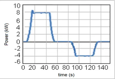
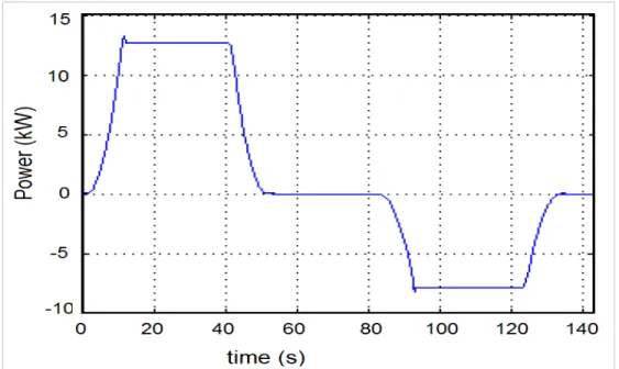
The trend of the power absorbed / generated by the lifting motor is the following:

Fig. 2.3: Absorbed/Delivered power of the lifting motor

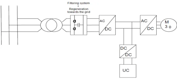
In Fig. 2.3 is presented the circuit that makes the system reversible and able to accumulate energy.

41

With this scheme the energy accumulated during the phases in which the loads behave generators (descending) can be returned at a later time with the dual benefit of energy saving and leveling of peak power consumption.

Starting from the three-phase grid, the power of the system is obtained by a bridge three-phase diode rectifier with capacitor on the dc-link that ensures a DC voltage on the dc-dc-link. The presence of appropriate filters in the input of the bridge rectifier ensures compliance with regulatory limits at the point of interconnection to the electricity distribution network.

The drive electric responsible for movement of the bridge crane consists of a three-phase induction motor with field oriented control, and a three-phase inverter.

The accumulation system, in this case a bank of ultracapacitors (UC: Ultracapacitor), supplies power to the electric drive during the lifting phase of the load (resulting in discharge of the UC)and recovers the energy that is available during the descending phase of the load (resulting in charging of the UC).

To interface the storage system with the link a bidirectional dc-dc step-up/step-down converter is required, which shall govern the storage and the return of power according to the logic of control that depend on the practical employment.

2.4

Gantry Crane System

The lifting system under consideration consists of a gantry crane with a capacity of 50 tons. In table 1 the main specifications are listed and in Fig. 4 the geometry of the gantry crane is presented.

42

Table 2: Main features of the lifting system

Maximum lift height (m) 15

Maximum Weight (tons)

(including the container) 67

Grid voltage (Vac) 1500 Vac, 3-Phase, 50Hz

Induction motor supply 400 Vdc / 400 Vac

Dc-link (Vdc) 500 Vdc

Fig. 2.5: Geometry of the system

The working cycle of the crane examined is composed of the working phases listed below:

1. Load lifting; 2. Load Rotation; 3. Load Translation; 4. Load Descending;

5. Gantry Crane Scroll (if necessary); 6. Return Path.

At the end of these work phases, the gantry crane returns back to the starting point (without container) and repeats the process. The

43

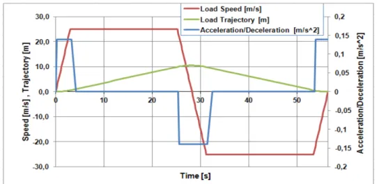
crane without the load at the point of return is much lower than this value. If it is needed to move the crane from the starting point to another point, the entire complex of the crane can be moved for a maximum distance of 500m. In Fig 5 and Fig.6 are shown the working phases of lifting and descending in terms of speed, acceleration, space (Fig. 5) and in terms of power, torque and energy (Fig.6). The total weight in the descending phase is 67t (including load).

Fig. 2.6: Load speed, trajectory and Acceleration during the lifting/descending process.

Fig. 2.7:Lifting/descending motor torque, energy, power during the lifting/descending process

44

The lifting-descending process lasts a total of 56 sec. A time pause between the two phases is not considered in the model. This comes at advantage of safety, because the presence of a pause improves the thermal behavior of the equipment.

As it can be seen, there is a power peak during the transition between the acceleration/deceleration phase and the regime phase. During the lifting process the expended energy is about 8650 kJ, while during the descending of the load the energy lost by the system is 5498kJ (Peak Energy – Final Energy). For the lifting process the peak power is about 459 kW.

In Fig.7 and Fig.8 is shown the work cycle referred to the rotation process of the load. The overall weight of the rotation set is 115t.

45

Fig. 2.9:Rotation motor torque, energy, power during the rotation process.

It was considered a maximum rotation of 180°. The rotation process endures maximum for 35s (180°). It has a peak power of 21 kW. The energy spent by the system during this process is about 490kJ.

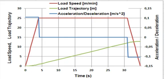
In Fig. 2.10 and Fig. 2.11 is shown the work cycle referred to the translation process of the load. This set has a total weight of 146t.

46

Fig. 2.11: Translation motor torque, energy, power during the translation process.

The maximum translation of the load is 48m, the peak power is 72 kW and the energy spent by the system during this process is 1391kJ.

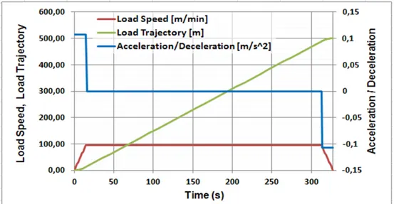
In Fig. 2.12 and in Fig. 2.13 is shown the work cycle referred to the scroll process of the entire crane with an overall weight of 198t.

47

Fig. 2.13: Scroll motor torque, energy, power during the scroll process.

The maximum scroll of the crane is 500m, the peak power is 114 kW and the energy spent by the system during this process is 34MJ.

The return procceses of rotation, translation and scroll were not shown in this paper because the return process is the same as the graphs that have been shown above. In this case the speed has to be considered negative and the weight with 50t less. That means the energy involved is lower.

2.5

Electrical system layout

Ultracapacitors (UC) show high power density and low energy density; they provide a cost-effective solution at medium power levels. UCs are widely used in applications that require high power peaks, in addition to an average energy consumption. In fact, by smoothing the power demand, it is possible an energy saving; this is particularly true in applications (like materials handling or hoisting machines) that allow to recover energy during braking or load descending. In Fig. 2.14 is shown the general block scheme of the electrical drive interfaced with UCs.

48

Fig. 2.14: Blocks scheme of the electrical drive

The UCs tank provides peak power supply to the electric motor, while it recovers (UCs recharge) the energy furnished by the traction drive itself during the descending of loads (regenerative braking).

A dc-dc converter is the interface between the storage unit and the dc-link; it has to be bidirectional in order to allow the current flows in both directions, according to UCs discharge or recharge cycle. The electrical scheme for the UCs bidirectional dc-dc converter is shown in Fig. 2.15.