Università degli Studi Roma Tre Scuola Dottorale in Geologia dell’Ambiente e
delle Risorse XXVIII Ciclo Sezione Geologia delleRisorse
Assessment of Soil Shaking Features in Urban Areas
PhD Student
Dott. Maurizio Piersanti
Tutor
Prof. Giuseppe Della Monica
Co-Tutor
Arrigo Caserta PhD
__________________________________________________________________________ 2
I
NDEX1. INTRODUCTION ... 5
1.1 OBJECTIVES OF THE PHDPROJECT ... 6
1.2 THESIS OUTLINE ... 7 2. GEOLOGICAL SETTINGS ... 9 2.1 GEOLOGY ... 9 2.2 MORPHO –TECTONIC ... 17 2.3 SEISMOLOGY ... 18 2.4 HYDROGEOLOGY ... 24 3. SEISMIC WAVES... 27 3.1 BODY WAVES ... 27 3.2 SURFACE WAVES ... 30
3.3 DISPERSION OF SURFACE WAVES ... 31
3.4 GENERAL SETTING ... 36
4. SITE EFFECTS ... 39
4.1 EFFECTS OF SOFT SURFACE LAYERS: THE AMPLIFICATION FUNCTION ... 40
4.2 SEISMIC NOISE ANALYSIS ... 44
4.2.1 Single Station Measurements ... 47
4.2.1.1 H/V Spectral Ratio and Body Waves ... 49
4.2.1.2 H/V Spectral Ratio and Ellipticity ... 50
4.2.1.3 H/V Spectral Ratio and Love Waves ... 52
4.2.1.4 H/V Spectral Ratio and Complex Wavefield: Results from Numerical Simulation ... 53
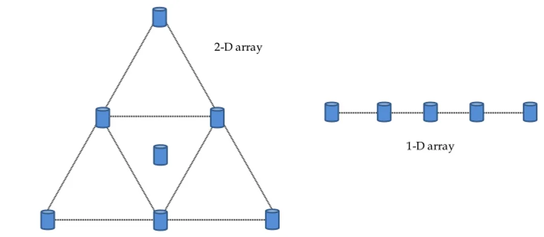
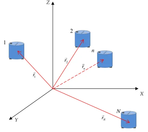
4.2.2 Array Analysis ... 54
4.2.2.1 The frequency-wavenumber Power Spectrum ( f-k Spectrum) ... 55
4.2.2.2 Conventional f-k Analysis (CVFK) ... 58
4.2.2.3 Capon’s Analysis (HRFK) ... 59
4.2.2.4 Array Geometry, Resolution and Aliasing ... 60
4.2.2.5 Array Transfer Function ... 62
4.2.2.6 Multichannel Analysis of Surface Waves (MASW) ... 65
4.3 SOIL BEHAVIOR UNDER CYCLIC STRESS ... 66
4.3.1 Resonant Column Test (RCT) ... 69
4.3.2 Cyclic Torsional Shear Test (CTS) ... 71
4.4 SOIL LIQUEFACTION ... 72
4.4.1 Testing Liquefaction Risk: Simplified Procedures ... 73
5. DATA ANALYSIS AND RESULTS ... 77
5.1 SEISMIC NOISE MEASUREMENTS:SINGLE STATION ANALYSIS ... 77
5.2 GEOGNOSTIC DRILLINGS ... 81
5.3 DOWN-HOLE TEST ... 85
5.4 SEISMIC NOISE MEASUREMENTS;ARRAY ANALYSIS ... 86
5.4.1 Site S5 ... 86
5.4.2 Site Piazza Haring ... 91
5.5 GEOLOGICAL RECONSTRUCTION OF THE STUDY AREA ... 95
5.5.1 Test Site Area ... 96
5.5.2 High Crati Valley Area ... 97
5.6 LABORATORY TESTS ... 98 5.6.1 Site S1 ... 99 5.6.2 Site S2 ... 100 5.6.3 Site S3 ... 101 5.6.4 Site S4 ... 102 5.6.5 Site S5 ... 103
__________________________________________________________________________ 3
5.6.6 Resonant Column and Cyclic Torsional Tests ... 105
5.7 TESTING LIQUEFACTION RISK ... 110
5.8 1DMODEL OF SEISMIC LOCAL RESPONSE AT SITE S5 ... 116
6. CONCLUSIVE REMARKS ... 121
6.1 AMBIENT VIBRATION ANALYSIS:H/V ... 121
6.2 BOREHOLES ... 121
6.3 AMBIENT VIBRATIONS ANALYSIS:SEISMIC ARRAYS ... 122
6.4 GEOLOGICAL RECONSTRUCTION OF THE CONTACT SEDIMENTARY COVERS-METAMORPHIC BEDROK ... 122
6.5 LABORATORY TESTS:TESTING LIQUEFACTION RISK... 122
6.6 LABORATORY TESTS:RESONANT COLUMN AND CYCLIC TORSIONAL SHEAR TESTS ... 123
6.7 1DMODELLING ... 123
6.8 FUTURE RESEARCH ... 124
ACKNOWLEDGMENTS ... 126
__________________________________________________________________________ 4
__________________________________________________________________________ 5
1. I
NTRODUCTION
The damages produced during moderate and large earthquakes are principally influenced by the interaction of seismic wavefield with the shallow subsurface geology and soil conditions. For this reason the degree of shake-ability of the ground during strong ground motion at locations with high vulnerability has been a matter of growing interest in seismological investigations dealing with seismic hazard analysis. Site amplifications in shallow unconsolidated sediments can be predicted using the theory of linear elastic wave propagation and computing S-wave resonances due to reverberation of seismic energy between the free surface and the sediment structure overlying a bedrock. The knowledge of the shallow shear wave velocity structure is essential for reasonable strong motion predictions at a given site. The assessment of soil shaking features in urban areas is crucial to quantify the expected local seismic response under strong motion conditions. During last decades many studies of this kind were conducted on some big cities (Fäh et al. 1997; Faccioli 1999; Jimenez et al. 2000; Raptakis et al. 2004; Panza et al. 2004; Ansal et al. 2010).
The city of Cosenza is located in the southern part of the Crati Basin in the Calabria region, geologically taken part of the Calabrian Arc. As well as the southern Apennines and eastern Sicily, it represents a very active tectonic area, in particular one of the most active area in the entire Mediterranean Region. Many geological studies were performed in the Crati Basin (Tortorici et al., 1995, Van Dijk et al., 2000, Spina et al., 2011, Tortorici et al., 2002), with the aim to reconstruct the actual stratigraphy of the area and to define its structural geological setting. The historical centre of Cosenza has been affected by numerous earthquakes during last years causing many damages to its architectural heritage; nevertheless, until now, no detailed geotechnical studies on the near-surface geology are available in literature. In order to fill this gap and better understand and quantify the expected ground shaking within the city of Cosenza, a multidisciplinary research project called pon-MASSIMO (http://openmap.rm.ingv.it/ponmassimo/) was carried on and a detailed analysis was made of the physical and mechanical properties of the different lithotypes constituting the recent sedimentary fill of Crati valley.
__________________________________________________________________________ 6 One of the purposes of the MASSIMO project is to study and monitor the response of different types of constructions to seismic stress by considering the near-surface geology, the topographic characteristics and the elastic properties of soils in relation to the monument architectural and static preservation. The selected Test Site is the Calabria Region (Italy), where some preliminary architectural constructions have been selected in three main urban areas, i.e. Cosenza, Vibo Valentia and Reggio Calabria. As mentioned before, this PhD thesis analyses in detail the urban area is the city of Cosenza.
1.1 Objectives of the PhD Project
The main purposes of this PhD dissertation are
Realize a geological reconstruction of the top of the bedrock
Assess possible site effects in the area of the Test Site chosen by the MASSIMO project: the San Agostino Church and the Monumental Complex of the
Bretti&Enotrii in the city of Cosenza;
The choice of the specific Test Site was made by the Cultural Heritage, considering its architectural and Historical importance for the city of Cosenza. The aforementioned purposes are reached by means of several techniques and different approaches, in particular inversion techniques in the context of ambient vibration methods in order to obtain vertical shear-wave velocity profiles and laboratory tests on sampled soils. A special attention has been paid to the reliability of the inverted profiles and to the possibility of including information from other types of experiments in the inversion process. The derivation of one-dimensional shear-wave velocity profiles from surface shear-wave dispersion curves is a classical inversion problem in geophysics, generally solved using linearized methods (see Tarantola for further readings). The inversion of dispersion curves is known to be strongly non-linear and affected by non-uniqueness, i.e. various models may explain the same data set with an equal misfit. During this thesis, we used the open source program GEOPSY (www.geopsy.org) which uses the Neighbourhood Algorithm (Sambridge, 1999a, 1999b, Wathelet et al, 2004, Wathelet, 2008) for inverting dispersion curves. The software allows the inclusion of prior information on the different parameters and a major effort has been made to optimize the computation time at the different stages of inversion, including frequency
__________________________________________________________________________ 7 information measured with the H/V technique. This has been necessary to design a geognostic drillings campaign, and to calibrate and compare the dynamic geological profiles.
1.2 Thesis Outline
This Doctoral Thesis has been organised in three different blocks. The first part describes the state of art of the geological knowledge of the Crati Basin, that is the regional context where the city of Cosenza is located. The second part is pure methodological: it tries to give an insight to the different methodologies used to evaluate site effects and to assess the dynamic behaviour of soils; great emphasis is given to the characteristics of surface waves and their use for site characterization. The remaining part presents the results of the application of the methods described and the relative conclusions.
Section 1 In this Section a geological overview of the Crati Basin and in
particular of the area of city of Cosenza is presented; such overview includes geological settings, morpho–tectonics, seismology and hydrogeology of the Crati Basin.
Section 2 Describes the characteristics of the seismic waves, both body
waves and surface waves; particular emphasis is given to the surface waves, especially to their dispersive characteristic and their use for site characterization.
Section 4 The concept of site effects is presented. More in detail the
techniques used to evaluate it are presented, including seismic noise analysis (Nakamura technique, seismic arrays), and laboratory tests (grain-size analysis, resonant column and cyclic torsional shear tests). The phenomenon of soil liquefaction is also introduced, including simplified techniques used to evaluate it.
Section 5 In this section all the results of the study are presented.
Section 6 Some comments and conclusions are summarised, together
with the indication of some specific topics, about which some further research efforts are needed in the future.
__________________________________________________________________________ 8
Le savant n'étudie pas la nature parce que cela est utile; il l'étudie parce qu'il y prend plaisir et il y prend plaisir parce qu'elle est belle. Si la nature n'était pas belle, elle ne vaudrait pas la peine d'être connue, la vie ne vaudrait pas la peine d'être vécue. Je ne parle pas ici, bien entendu, de cette beauté qui frappe les sens, de la beauté des qualités et des apparences; non que j'en fasse fi, loin de là, mais elle n'a rien à faire avec la science; je veux parler de cette beauté plus intime qui vient de l'ordre harmonieux des parties, et qu'une intelligence pure peut saisir.
The scientist does not study nature because it is useful to do so. He studies it because he takes pleasure in it, and he takes pleasure in it because it is beautiful. If nature were not beautiful it would not be worth knowing, and life would not be worth living. I am not speaking, of course, of the beauty which strikes the senses, of the beauty of qualities and appearances. I am far from despising this, but it has nothing to do with science. What I mean is that more intimate beauty which comes from the harmonious order of its parts, and which a pure intelligence can grasp.
Jules Henri Poincaré
__________________________________________________________________________ 9
2. G
EOLOGICAL
S
ETTINGS
The city of Cosenza is located in the southern part of the Crati river Valley, a Plio-Pleistocene asymmetric half-graben with a N-S trend in the southern part and a SW-NE trend in the northern part, delimited on eastern side by the Sila Mountains and on South and West by the Catena Costiera (Figure 2.1). The graben is filled by Tertiary and Quaternary (from Late Miocene up to Present) clastic deposits (essentially gravels, sands and clays) overlying a Palaeozoic metamorphic bedrock. Considering the aim of this work the geological succession of the Crati Basin and in detail of the urban area of Cosenza can be divided in two different groups: 1. Sedimentary covers: they are represented by marine deposits, composed of basal beige-clear sand and silt formation, blue clay formation and brown sand and conglomerate formation interbedded with levels of gravel, and alluvial deposits of Crati river and its tributaries.
2. Metamorphic bedrock: it is formed by different lithologies, such as biotite garnet-biotite gneiss and schists with acid intrusive complex (quartzdiorite, quartzmonzonite, granodiorite and granite); often, granitic outcrops are intruded into metamorphic rocks.
2.1 Geology
As mentioned above, the city of Cosenza is located in the southern part of the Crati river Valley. The Crati Basin is a tectonic depression (graben) located in the western sector of northern Calabria, geologically representing part of the Calabrian Arc. In the frame of the Mediterranean mobile belt, the Calabrian Arc is an arc-shaped continental fragment located between the E-W trending Sicilian Maghrebides, to the South, and the NW–SE trending Apennines, to the North. The Calabrian Arc (Figure 2.1) consists of a series of thrust nappes composed of tectonic units deriving from the deformation of different palaeo-geographic domains (Spina et al., 2011).
__________________________________________________________________________ 10 Figure 2.1 (a) Digital elevation model showing main strike-slip faults and extensional basins of the southern Apennines and northern Calabria. Major strike-slip fault zones: Pollino Fault Zone (PFZ), Petilia-S.Sosti Fault Zone (PSSFZ), Falconara-Cosenza Fault Zone (FCFZ), Amantea-Gimigliano Fault Zone (AGFZ), S.Nicola-Rossano Fault Zone (SRFZ). (b) Geological sketch of northern Calabria. (c) Topographic section across the Crati Basin, the Coastal Range and the Sila Massif (From Spina et al., 2011).
__________________________________________________________________________ 11 The backbone of the Calabrian Arc is composed of Palaeozoic crystalline rocks, which have been interpreted either as basement units belonging to the African continental margin or as part of the European palaeo-margin. Since the Oligocene, these basement rocks thrusted onto ophiolite-bearing units of the Neotethys domain. Since the Early Miocene, the whole tectonic edifice over-thrusted carbonate platform rocks of the Apulian continental margin.
The progressive migration of the Calabrian Arc towards the southeast occurred, since Middle Miocene times, along a NW–SE to WNW–ESE-trending regional strike-slip fault system characterized by left- and right-lateral movements in the northern and in the southern sector of the Calabrian Arc, respectively. Such faults, dissecting the pre-existing thrust sheets, played an important role in the Neogene-Quaternary geodynamic evolution of the Central Mediterranean area. Based on structural studies supported by seismic and bore-hole data, Van Dijk et al. (2000) proposed that the whole tectonic system consisted of Middle Miocene–Early Pleistocene crustal transpressional fault zones, mainly dipping towards the NE, characterized by left-lateral and reverse kinematics. Along these structures, in correspondence of their restraining bends, extrusion of the deep-seated units of the Calabrian Arc together with underlying Mesozoic carbonate rocks have been recently described by Tansi et al. (2007). Since the Middle Pleistocene, a strong regional, still active uplift affected the northern Calabrian Arc. This has been interpreted as the isostatic response to the removal of the high-density mantle/ lithosphere root, due to detachment of the Ionian subducted slab. The Crati Basin, forming part of this zone, is bounded by the Coastal Range to the west, by the Sila Massif to the east, and by the Pollino Ridge to the north (Figure 2.2). The basin is morphologically asymmetric with a steeper and shorter fluvial drainage along its eastern border, and the Crati River flowing along the easternmost side of the valley.
The Crati Basin is filled by Upper Miocene to Holocene clastic marine and fluvial deposits covering the Palaeozoic crystalline bedrock, in the southern part of the basin, and Meso - Cenozoic carbonates in its northern sector (i.e. in the Pollino area). The original stratigraphic contact between the basin infill and its bedrock is still well exposed all along the western side of the Sila Massif. Although the main depocentre is located in the northernmost sector of the basin (Sibari Plain), the thickness of the deposits increases from the Coastal Range towards the Sila foothills. Published stratigraphic data are mainly from specific sectors of the basin;
__________________________________________________________________________ 12 however it has been proposed that the whole basin fill consists of two main depositional sequences bounded by a regional angular unconformity. The first sequence, Late Miocene to Early Pliocene in age, is characterized in the structural highs by a Messinian unconformity, whereas the second one, spanning from the Middle-Late Pliocene to the Pleistocene, is represented by distinct lithofacies grading one into another both vertically and laterally.
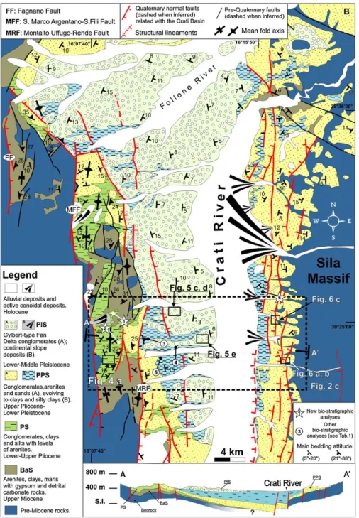
Figure 2.2 Geological maps of the Southern and Central sectors of the Crati Basin (From Spina et al., 2011).
__________________________________________________________________________ 13 The city of Cosenza is part of Sheet n° 236 - I NO the Geological Map of Italy (see Figures 2.3a, 2.3b); in the southernmost part of Crati river Basin the lithologies encountered in the area are:
Units of Gneiss, para-gneiss and biotitic-garnetiferous schistes (sbg) - Form
the basis upon which the various sedimentary units; this complex, rarely outcropping in the urban area of Cosenza, consists of para-gneiss and biotitic schists, often with garnets visible to the naked eye, with frequent injections of granitic material from fine-grained to coarse-grained. The condition of considerable mechanical loosening, evidenced by the numerous and often approximated lines of discontinuity, promotes the disruptive action and chemical alteration of atmospheric agents, and therefore, the formation of debris and alteration coverage present over most of surface outcrop of the formation. The permeability is generally low, with substantial increase in degraded and fractured areas. The processes of alteration and degradation tend to decrease with depth and the thickness of the altered material is usually minimal in areas subject to intense erosion (like the engravings valleys and slopes with steepness greater than 35%), while it reaches a maximum of a few tens of meters in the less steep and with plenty of water circulation. Therefore, in relation to different physical-mechanical behaviour, in the areas of outcrop of the formation, from ground level down, it is necessary to distinguish the following levels: - Angular pebbles of various sizes set in a sandy matrix containing clay and topsoil, at higher surface; - Rocky mass with degraded areas, at this level fractures tend to be filled by fine materials transported by water circulating; - Compact bedrock. The geotechnical behaviour of the geological formation is strictly depending on the state of continuity and alterations of the same: where the rock is fresh presents a high erosion resistance and low permeability, where instead is altered and degraded presents high permeability and low resistance to erosion.
Units of Sands (PS2-3; PS3) - This geological formation is more widespread
within the urban area. The complex consists of clear brown to medium-grained sands, sometimes through a micro-conglomerates. The formation is intercalated with thin layers of silty-clay and gravel lenses with polygenic elements. The upper part of the series in many cases is mainly composed of gravels, sands
__________________________________________________________________________ 14 and conglomerates subject. The complex is generally compact and has a moderate resistance to erosion. Its permeability is generally high.
Units of Clays, Silty Clays (Pa3; Pa2-3) - The clays of this unit are light gray
coloured. They look to be massive to thinly laminated, locally interbedded light brown silt layers, sometimes containing, up to the roof of the sequence, interbedded conglomerates and sands. Pass gradually upwards to sands with intercalated layers of clayey and sandy. The erosion resistance of the formation is poor and low permeability.
Unit of Conglomerates (Pcl3) - Constitute the major summit of the slopes of the
hill of the municipality, in fact, can be traced along the axes of erosion of many small valleys. The formation outcrops mainly in the hydrographic right of the River Crati along the section before Sila, even at altitudes higher than 600/700 m above sea level. The sequence consists of conglomerates rich in matrix coloured red and pink, with elements of various sizes, up to decimetre, little rounded and surrounded by coarse sandy matrix. The elements that constitute the conglomerates have a variable composition from area to area: in general, consist essentially of granitic, phyllites and sedimentary rocks together, in other cases only gneissic rocks. Locally, the transition to the underlying sand is gradual and occurs by intercalation of sandy and conglomeratic levels. The complex is generally well compacted and has a good resistance to erosion. The permeability is high.
Conglomerates of ancient alluvial river terraces (qcl) - Represent the substrate
support of the entire new city, starting from the confluence of Crati and Busento River and reaching the Campagnano Torrent. The deposits mainly consist of non-cemented gravel with sandy or clayey matrix with interbedded lenses of coarse grained sand and/or polygenic conglomerates. The thickness is generally of a few meters. The total deposits are quite constipated and have a moderate resistance to erosion. The permeability is medium to high and is a function of the particle size of the sediment.
Floods (a, f) – They constitute a considerable part of the terrains in the area of
study, characterized by materials deposited during the various floodings of the River Crati that have occurred relatively recently (Holocene). The deposits are gravelly/sandy/silty/clayey continental deposits, now stabilized and secured. The lithological variability, even in the short surroundings, is their most
__________________________________________________________________________ 15 obvious feature, depending on their formation by fluvial dynamics. Thicknesses are slightly constipated and highly permeable.
Recent Deposits (ac) - Represent the deposits of loose beds of river plain,
consist of gravel and sand in earthy matrix.
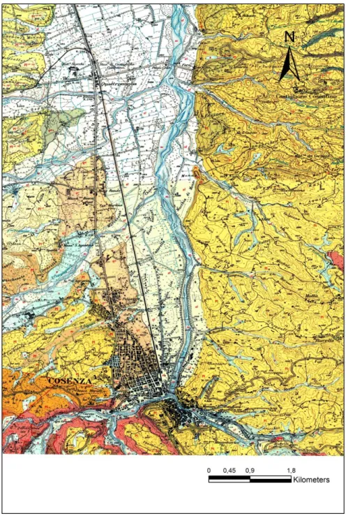
Figure 2.3a Geological map of the Crati Basin processed with ArcGis software, including Sheet n° 236 - I NO (Cosenza), and Sheet n° 229 - II SO (S. Pietro in Guarano).
__________________________________________________________________________ 16 Figure 2.3b Legend of the Geological Map.
__________________________________________________________________________ 17
2.2 Morpho – Tectonic
The Crati Basin is part of a series of basins located along the Tyrrhenian side of the Calabrian Arc. According to Monaco and Tortorici (2000), these basins (including the Mesima and Gioia basins) are part of the Siculo-Calabrian Rift Zone, a sector undergoing crustal extension where basin-bounding normal faults produced strong (M≥6.5) historical earthquakes and still release seismic energy. The extensional basins are segmented by long-lived, NW–SE striking left-lateral fault zones. The various basin segments exhibit different trends. Although the recent tectonic evolution of these basins is generally accepted by most of the authors, as it was previously mentioned, their structural style and tectonic setting are still strongly debated.
__________________________________________________________________________ 18 The southern portion of the graben of the Crati Basin, geographically corresponding to the Catena Costiera-Crati Valley-Sila Plateau element, is bounded on the West and East, from stair casing normal faults systems, oriented N-S and lowered to the Crati river, culminating for discards and extension, respectively, with the lines "San Marco Argentano-San Fili" and "Rogliano-Bisignano." The faults, belonging to the N-S system, are connected to a extensional tectonics stage with axes of maximum extension oriented ESE-WNW, lasted from upper Pliocene until the end of the Pleistocene, particularly intense from the Middle Pleistocene, and is still active, as evidenced by the intense seismic activity in the region.
The northern part of the graben is more complex and characterized by two systems of normal faults, trending WNW-ESE and NE-SW. The first is inherited from a previous left strike slip band, of regional significance (Pollino Line) that has developed on the border between Calabria and Basilicata valley during the lower-middle Pleistocene. During the late Pleistocene extensional stages, these faults have been reactivations "in normal".
In the Crati valley, the fault system WNW-ESE is the director of "San Sosti-Luzzi," which marks the transition between the southern and northern part of the graben, and the lineation of "Spezzano Albanese-Cirò Marina" (Fault of Rossano) that delimits the northern outcrop of the crystalline-metamorphic units outcropping in the Sila Plateau. As for the faults that make up the Pollino Fault, these guidelines also show evidence of double kinematic mechanism.
The system of NE-SW normal faults is less evident and finds its highest expression in Sangineto Line which skirts the Crati graben to the N-W. Various authors attribute an important role in the geodynamic structure: the formation of the Crati basin is in fact attributed to the activity of left strike slip of Sangineto Line. Even the faults belonging to the system NE-SW have been reactivated by Quaternary tectonics associated with the late extensional phase.
2.3 Seismology
The Calabrian Arc, as well as the southern Apennines and eastern Sicily, represents a very active area, in particular one of the most active area in the entire Mediterranean Region, characterized by historic crustal events, the largest of which reached (in the latest 6 centuries) an MKS intensity of X – XII ( 6M7.1), and by
__________________________________________________________________________ 19 the occurrence of intermediate and deep focus earthquakes located along the inner side of the arc, beneath the southern Tyrrhenian sea. The occurrence in the Calabrian Arc of both intense Quaternary faulting and active crustal seismicity suggest that these phenomena must be related to each other. Events of high intensity (I = IX-X MCS) have repeatedly affected the territories of Cosenza (1835, 1854, 1870), Bisignano (1184, 1887) and Roggiano Gravina (1913).
The city of Cosenza has been affected by numerous earthquakes, such as the earthquakes of 12 October 1835, with maximum intensity (Intensity X) in Castiglione Cosentino, 12 February 1854 (Intensity X in Donnici) and 4 October 1870 (Intensity X in Mangone). Cosenza and its surroundings tend to be severely affected by shocks even with its epicenter in nearby areas, as evidenced by the reconstruction of the effects of the earthquakes of 27 March 1638 and 8 September 1905.
In order to characterize the historical seismicity of the city of Cosenza the "Catalogue of strong earthquakes in Italy from 491 BC to 1997" - CFTI, “Parametric
Catalog of Italian earthquakes" (http://storing.ingv.it/cfti4med/, the "Italian
macroseismic database" (http://emidius.mi.ingv.it/CPTI11/) and DBMI11 (http://emidius.mi.ingv.it/DBMI11/), "Catalogue of the Italian Seismicity, 1981 to 2002” - CSI 1.1 were consulted. All these database are provided by INGV (Istituto
Nazionale di Geofisica e Vulcanologia, Italy, http://terremoti.ingv.it/it/).
I[MCS] Data Ax Np Io Mw
9 1184 05 24 Valle del Crati 6 9 6.74 ±0.44
7 1556 11 17 COSENZA 1 7 5.14 ±0.34 8-9 1638 03 27 15:05 Calabria 213 11 7.03 ±0.12 8 1638 06 08 09:45 Crotonese 42 10 6.89 ±0.25 HD 1656 06 Calabria, Cosenza 1 7-8 5.35 ±0.34 5 1659 11 05 22:15 Calabria centrale 126 10 6.55 ±0.13 4 1693 01 08 22:15 Calabria settentrionale 8 8 5.67 ±0.69 5 1738 06 Pizzo (VV) 4 6-7 4.93 ±0.34 F 1743 02 20 16:30 Basso Ionio 77 9 7.13 ±0.19 5-6 1744 03 21 20:00 Crotonese 29 8 5.74 ±0.44
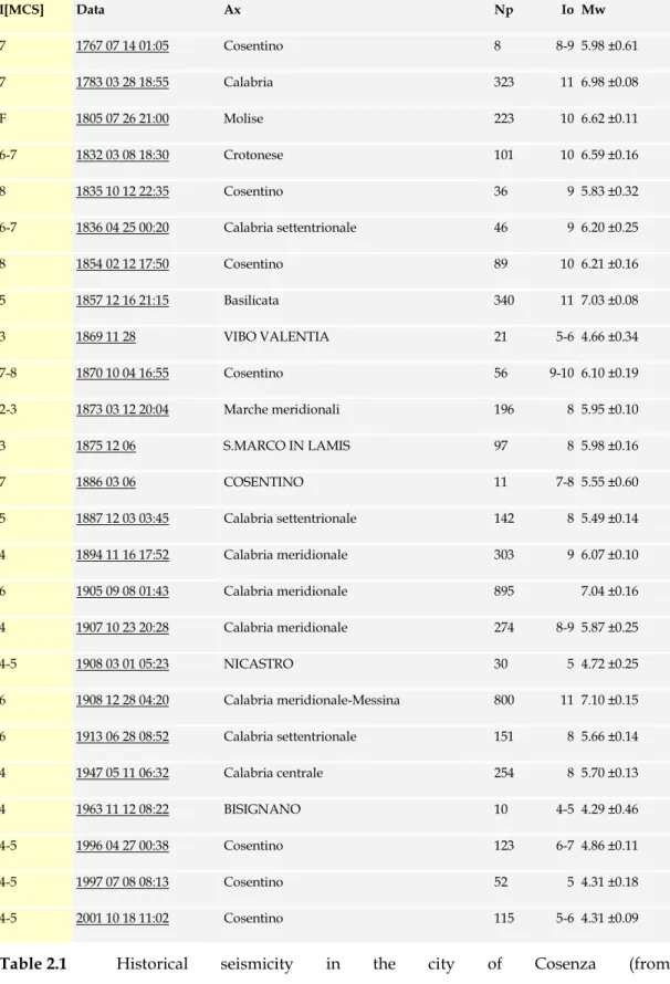
__________________________________________________________________________ 20 I[MCS] Data Ax Np Io Mw 7 1767 07 14 01:05 Cosentino 8 8-9 5.98 ±0.61 7 1783 03 28 18:55 Calabria 323 11 6.98 ±0.08 F 1805 07 26 21:00 Molise 223 10 6.62 ±0.11 6-7 1832 03 08 18:30 Crotonese 101 10 6.59 ±0.16 8 1835 10 12 22:35 Cosentino 36 9 5.83 ±0.32 6-7 1836 04 25 00:20 Calabria settentrionale 46 9 6.20 ±0.25 8 1854 02 12 17:50 Cosentino 89 10 6.21 ±0.16 5 1857 12 16 21:15 Basilicata 340 11 7.03 ±0.08 3 1869 11 28 VIBO VALENTIA 21 5-6 4.66 ±0.34 7-8 1870 10 04 16:55 Cosentino 56 9-10 6.10 ±0.19 2-3 1873 03 12 20:04 Marche meridionali 196 8 5.95 ±0.10 3 1875 12 06 S.MARCO IN LAMIS 97 8 5.98 ±0.16 7 1886 03 06 COSENTINO 11 7-8 5.55 ±0.60 5 1887 12 03 03:45 Calabria settentrionale 142 8 5.49 ±0.14 4 1894 11 16 17:52 Calabria meridionale 303 9 6.07 ±0.10 6 1905 09 08 01:43 Calabria meridionale 895 7.04 ±0.16 4 1907 10 23 20:28 Calabria meridionale 274 8-9 5.87 ±0.25 4-5 1908 03 01 05:23 NICASTRO 30 5 4.72 ±0.25 6 1908 12 28 04:20 Calabria meridionale-Messina 800 11 7.10 ±0.15 6 1913 06 28 08:52 Calabria settentrionale 151 8 5.66 ±0.14 4 1947 05 11 06:32 Calabria centrale 254 8 5.70 ±0.13 4 1963 11 12 08:22 BISIGNANO 10 4-5 4.29 ±0.46 4-5 1996 04 27 00:38 Cosentino 123 6-7 4.86 ±0.11 4-5 1997 07 08 08:13 Cosentino 52 5 4.31 ±0.18 4-5 2001 10 18 11:02 Cosentino 115 5-6 4.31 ±0.09
Table 2.1 Historical seismicity in the city of Cosenza (from http://emidius.mi.ingv.it/DBMI11/): I is the intensity resented in the city of Cosenza, Np
is the number of points of intensity (locations affected by the event), I0 is the epicentral
__________________________________________________________________________ 21 Another important means used to characterize the seismicity of the Crati Basin is the DISS, (Database of Individual Seismogenic Sources - INGV, http://diss.rm.ingv.it/diss/) through which three individual seismogenetic sources have been defined in the study area. An individual seismogenic source is defined by geological and geophysical data and is characterized by a full set of geometric (strike, dip, length, width and depth), kinematic (rake), and seismological parameters (single event displacement, magnitude, slip rate, recurrence interval). Each parameter is then rated for accuracy. Individual seismogenic sources are assumed to exhibit strictly-periodic recurrence with respect to rupture length/width, slip per event, and expected magnitude. They are compared to worldwide databases for internal consistency in terms of length, width, single event displacement and magnitude, and can be augmented by fault scarp or fold axis data when available (usually structural features with documented Late Pleistocene – Holocene activity).
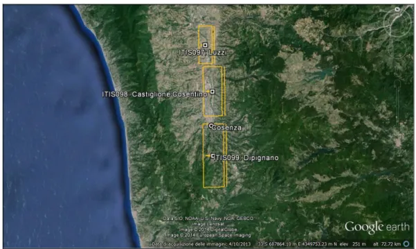
The three individual seismogenetic sources defined in the Crati Basin are shown in the Figure 2.5:
Figure 2.5 Location of the individual seismogenetic sources defined in the Crati Basin (from http://diss.rm.ingv.it/diss/).
Luzzi Source: it is based on data regarding the recent tectonic activity of the
southern sector of the Crati Valley constrained by the occurrence of the 14 July 1767 earthquake (Mw 5.8). Luzzi Source is located along the eastern side of the
__________________________________________________________________________ 22 valley, between the Mucone River and the Caprio Creek. The drainage pattern shows that the Crati River flows closer to the eastern side of the Valley, thus suggesting a possible active subsidence of that side of the valley. The geometry of this source has been constrained mainly by geological and geomorphological observations, in particular the drainage pattern and the deformation of the top of the metamorphic substratum along with the overlying Pleistocene units, highlighted by Carobene and Damiani (1985). The location of this source is constrained to the south by the occurrence of another Mw 5.9 earthquake on 12 october 1835 (CPTI, 2004). The following geometrical parameters are proposed for the source: the strike (N180°) is chosen according to that of Crati Valley fault system; the fault dips 65° towards the West, according to geological and geomorphological data; the rake is assumed to be 270° (pure normal faulting), based on geodynamic considerations and focal mechanisms of the area; the length (7.6 km) is constrained by the geological section of Carobene and Damiani (1985) and by scaling relationships with the 1767 earthquake magnitude; the down-dip width (6.3 km) is obtained by scaling relationships. Maximum macroseismic intensity of the 1767 earthquake was VIII-IX and the macroseismic epicenter is located about 12 km north of Cosenza, near the Caprio Creek (DBMI04, Stucchi et al., 2007). The location of Luzzi Source is consistent with the location of the highest damage, and fit well the macroseismic pattern that suggests the activation of a shallow source.
Castiglione Cosentino Source: it is located along the eastern side
of the valley, in the southernmost portion of it. The geometry of this source is constrained by geological and geomorphological observations, in particular the drainage pattern and the distribution of the radon anomalies in the area. The drainage pattern shows that the Crati River flows closer to the eastern side of the Valley, thus suggesting a possible active subsidence of that side of the valley. The orientation of the N-S trending normal fault shows a clear correlation with the geometry of radon anomalies in soil gas (according to Tansi et al., 2005b). The location of Castiglione Cosentino Source is constrained to the north by the occurrence of another Mw 5.8 earthquake on 14 July 1767 (CPTI, 2004), and to the south by the presence of a transverse structure known in literature as Vette Line. This lineament was the locus of a series of earthquakes with
__________________________________________________________________________ 23 magnitude between 4 and 5 that occurred in the nineteenth and twentieth centuries (CPTI, 2004). Another event having a Mw 5.2 (CPTI, 2004) took place in 1556 along the Vette Line. Maximum macroseismic intensity was X and macroseismic epicenter is located immediately NE of Cosenza (DBMI04, Stucchi et al., 2007). Macroseismic field of the 1835 event is consistent with the geometry of the proposed shallow source. We propose the following geometrical parameters for the source: the strike (N180°) is chosen according to that of Crati Valley fault system; the fault dips 60° towards the West, according to geological and geomorphological data; the rake is assumed to be 270° (pure normal faulting), based on geodynamic considerations and focal mechanisms of the area; the length (10 km) and the down-dip width (7.5 km) are constrained by scaling relationships with the 1835 earthquake magnitude.
Dipignano Source: it is based on data regarding the recent tectonic activityof the southern sector of the Crati Valley constrained by the occurrence of the 12 February 1854 earthquake (Mw 6.1). The geometry of this source is constrained mainly by geological and geomorphological observations. The location of this source is constrained to the north by the occurrence of another Mw 5.9 earthquake on 12 october 1835 (CPTI, 2004), and by the presence of well-known Vette Line. This transverse structure was the locus of a series of earthquakes with magnitude between 4 and 5 that occurred in the nineteenth and twentieth centuries (CPTI, 2004). Another event having a Mw 5.2 (CPTI, 2004) took place in 1556 along the Vette Line. The following geometrical parameters for the source are proposed: the strike (N180°) is chosen according to that of Crati Valley fault system; the fault dips 62° towards the West, according to geological and geomorphological data; the rake is assumed to be 270° (pure normal faulting), based on geodynamic considerations and focal mechanisms of the area; the length (12.7 km) is constrained by scaling relationships with the 1854 earthquake magnitude; the down-dip width (6.3 km) is obtained by scaling relationships. Maximum macroseismic intensity was X and macroseismic epicenter is located immediately NE of Cosenza (DBMI04, Stucchi et al., 2007). Macroseismic field of the 1854 event is consistent with the geometry of the proposed source.
__________________________________________________________________________ 24
2.4 Hydrogeology
The Crati River and its tributaries, within the hydrogeological basin of Sybaris, is the most important hydrographic system of the Calabria region. From the southern part of the basin, Crati flows exactly South-North up under Tarsia; there turns North-East and flows into the Ionian Sea (Figure 2.6).
Legend
Crati Basin Crati River
Ionian Sea Tyrrhenian Sea
Figure 2.6 Crati river in relation to its homonymous Basin .
The Crati is fed by many tributaries, some of which descend to the East or North-East from the western mountain range, while others flow out from the Sila. In the southern part of the Sila streams flow out mainly to the west; the northern part instead feeds a number of streams that flow to the northeast: some of these reach the Crati in its lower course, others go directly to the Ionian Sea. The drainage of the western flank of the western mountain range is made by rivers that descend to the west to the Tyrrhenian Sea.
The analysis of the piezometric surfaces (Celico et al., 2000) allowed to detect, at large scale, in the field of high and medium Crati Valley, the presence of an axis of preferential drainage groundwater, coinciding precisely with the riverbed of the Crati river (Cassa per il Mezzogiorno, 1977), whereas in the lower Crati Valley (the Plain of Sybaris), the changes in areas iso-piezometrics lets you highlight, along the northwestern sector, the presence of substantial water supplies from the carbonate massif of Pollino through the Plain of Castrovillari.
__________________________________________________________________________ 25 On the right bank of the Crati river it is clear the presence of axes drainage preferential headed to the coastal zone.
The knowledge of the terrain permeability features and the study of depositional sequences in the study area allowed to identify two main types of aquifers:
1. Sila aquifers: they are hosted in acid intrusive complex and in biotite and garnet-biotite gneiss and schist rocks (sbg);
2. Crati river Valley aquifers: hosted in Plio-Pleistocene sandy-gravelly-conglomeratic deposits and in Holocene alluvial deposits. These aquifers are laterally and vertically limited by impermeable Plio-Pleistocene clayey-sandy deposits.
The aquifers of the Crystalline basement are deeper and highly productive, whereas those of the Crati river Valley are more superficial and have less capacity; the crystalline basement hosts, in fact, represent a regional aquifer with a good lateral continuity. It is probable that there is a groundwater-streamwater exchange active system between the water body of crystalline basement and that occurring in the alluvial deposits. On the contrary, in the latter a series of small suspended and overlapped groundwater bodies have been characterized; they are stored in the gravel and sand levels and they seem to constitute a multilayer aquifer. The dimension and the hydraulic potential of these groundwater bodies vary with the not well-known horizontal extension of the layers in which they are stored, but probably the potentiality is limited for their low permeability. The blue clay formation represents the aquiclude level. These aquifers are however located below the riverbed and therefore presumably the river feed the groundwaters. The features of these aquifers depend also on the structural-geological settings. In fact, an active fault alignment puts into contact the post-orogenic formations with the crystalline bedrock, constituting a preferential way of infiltration and transfer of the water. However, the basement groundwater circulation is very articulated and that is also due to the heterogeneity of these rocks. Beneath the alluvial deposits, in beige clear sand and silt formation, it is probable the presence of a regional aquifer separated from the overhanging water bodies by the Plio-Pleistocene clays.
Further investigations may be aimed to define the possibility of likely connection among the Crati river valley aquifers and those hosted in the Crystalline basement and the existence of possible drainage processes between them.
__________________________________________________________________________ 26
__________________________________________________________________________ 27
3. S
EISMIC
W
AVES
Seismic waves can be divided into progressive and standing waves. Progressive seismic waves propagate away from seismic sources; standing seismic waves, also known as free oscillation of the Earth, represent vibrations of the Earth as a whole; in particular, this kind of waves are generated by strong earthquakes.
From the point of view of the spatial concentration of energy, waves can be divided into body waves and surface waves. Body waves can propagate into the interior of the corresponding medium, whereas surface waves are concentrated along the surface of the medium. Note that instead of surface waves we should rather speak of a broader category of guided waves: guided waves can propagate along the surface of a medium (surface waves), along internal discontinuities, or other waveguides.
In this Chapter an overview of the main characteristics of the seismic waves is presented; particular emphasis is given to the surface waves, and their use site characterization.
3.1 Body Waves
The theory of the elasticity explains that there are two types of elastic body waves: 1. Longitudinal waves, also called compressional, dilatational or irrotational waves.
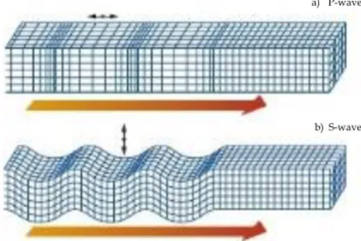
In seismology they are also known as P waves (primary waves), because they represent the first waves appearing on seismograms. This waves involve compression and rarefaction of the material as the wave passes through it, but not rotation. Every particle of the medium, through which the wave passes, vibrates about its equilibrium position in the direction in which the wave travels.
2. Transverse waves, also called shear, rotational or equivoluminal waves. In seismology, they are also called S waves (secondary waves). These waves involve shearing and rotation of the material as the wave passes through it, but
__________________________________________________________________________ 28 not volume change. The particle motion is perpendicular to the direction of the propagation of the wave.
Consider the equation of motion for a homogeneous isotropic medium without body forces:
2 2 2 u u u t ,where λ and μ are the Lamé coefficients, and ρ is the density (coefficient μ is the shear modulus). Assume that the displacement vector field u u u v w
, ,
is continuous with its first derivates. For the Helmholtz theorem this vector can be decomposed into irrotational and solenoidal parts (Graff, 1975):u ,
In previous expression is the scalar potential, and is the vector potential. By inserting this expression into the equation of motion and interchanging the order of some operation, we obtain
2 2 2 2 2 2 2 2 1 1 2 t t The above equation will be satisfied if the expressions in the square brackets are constants. In a special case, when these constants are zero, we arrive at the wave equations 2 2 2 2 2 2 2 2 1 , 1 t t , where 2 ,
are the longitudinal and transverse wave velocities, respectively. This means that the scalar equation describes longitudinal waves, and the vector wave equation describes transverse waves.
Both longitudinal and transverse waves can propagate in solid media. However, only longitudinal waves can propagate in fluids, cause for this state of matter μ=0, consequently, β=0.
__________________________________________________________________________ 29 Assume now that the displacement vector is independent of the y-coordinate; this means that, at a given time, the wave parameters are constant along any line which is parallel to the y-axes. This situation occurs, for example, if a plane wave with a constant amplitude propagates in a arbitrary direction in the
x z, -plane. Following Novotny (1999), the wave field can be decomposed into two parts; thus, we can express vector potential as a sum of two vectors,SV SH where
0, ,0 ,
,0,
SV y SH x z the displacement vector can be expressed as P SV SH u u u where
,0, 0, ,0 . P SV SV SH SV u u w u v Vector uP SV represent a wave motion polarized in the
x z, -plane and consistingof a longitudinal wave (P wave, described by potential ) and a transverse wave polarized in this vertical plane (SV wave, described by potential y).
Vector uSHrepresents a transverse wave polarized in the horizontal plane parallel to the y -axis.
a) P-wave
b) S-wave
__________________________________________________________________________ 30
3.2 Surface Waves
As suggested by the name, surface waves propagate along the surface of a medium. They are very important in seismology because they represent the principal phase of seismograms. There are two different types of surface waves: 1. Rayleigh waves. These waves are elliptically polarized in the plane which is
formed by the normal to the surface and by the direction of propagation (Rayleigh, 1985). Near the surface of a homogeneous half-space, the particle motion is a retrograde vertical ellipse (anticlockwise for a wave travelling to the right).
2. Love waves. The particle motion in these waves is transverse and parallel to the surface. As opposed to Rayleigh waves, Love waves cannot propagate in a homogeneous half-space. Love waves can propagate only if the S-waves velocity generally increases with the distance from the surface of the medium. The simplest medium in which Rayleigh waves can propagate is a homogeneous isotropic half-space, whereas the simplest model in which Love waves can propagate is a homogeneous isotropic layer on a homogeneous isotropic half-space. Their amplitude decreases exponentially with the depth, and most of the energy propagates in a shallow zone, roughly equal to one wavelength. The solicited zone is so bounded in depth, and consequently the wave propagation is influenced by the properties of this limited portion of soil. Surface waves do not represent principally new types of waves, but only interference phenomena of body waves (Novotny, 1999). Considering their importance, a great detail will be given to this type of elastic waves.
a) Rayleygh wave
b) Love wave
Figure 3.2 The particle motion for surface waves: a) Rayleigh waves and b) Love waves.
__________________________________________________________________________ 31
3.3 Dispersion of Surface Waves
As mentioned in the Introduction one of the main objective of this doctoral thesis is the derivation and the inversion of the dispersion curves of the Rayleigh waves recorded by ambient vibrations to get the shear-wave profile of the study site. In general terms we speak of the dispersion of waves if their velocity depends on frequency (Novotny, 1999; Foti, 2000). All surface waves, except Rayleigh waves in an isotropic half-space, exhibit dispersion, with the apparent velocity along the surface depending on frequency (Novotny, 1999).
Before explaining the dispersion of surface waves we have to introduce two important quantities for general propagating waves in a medium: the group velocity and phase velocity.
Consider two plane harmonic waves of angular frequencies 1 and 2 propagating along the Cartesian x -axis at velocity c1 and c2; for simplicity assume both waves to be of same amplitude A . Denote by u1 and u2 the displacements of these waves, so we have:
1 sin 1 / 1 , 2 sin 2 / 2
u A t x c u A t x c .
Introducing the wavenumbers k11/c1 and k22/c2 the individual waves can be expressed as
1 sin 1 1 , 2 sin 2 2
u A t k x u A t k x .
The superposition of the two waves can be expressed as
1 2 1 2 1 2 1 2
1 2 2 sin 2 2 cos 2 2
k k k k
u u u A t x t x
.
Assuming close frequencies and wavenumbers
1 1 2 2 , , , , k k k k k k we then obtain
envelope2 sin cos 2 cos k sin
u A t kx t kx A t x t kx .
__________________________________________________________________________ 32 U k .
In the limiting case for small and k , we obtain the important formula
d U
dk
.
Velocity U is called group velocity. In our case, this is the velocity of propagation of the envelope of the two harmonic waves. This velocity is generally different from velocity c/k which is called the phase velocity. We can summarizes these results as follows: the individual peaks and troughs of the resulting wave (extending to a large or a finite number of propagating waves) propagate at the phase velocity, whereas their envelope propagates at the group velocity; generally the group velocity is the propagation of energy.
A transient wave (a wave of finite duration) do not change its shape during propagation in a dispersive medium because its individual spectral components (Fourier harmonics) propagate with the same phase velocities; in this case phase velocity and group velocity coincide. If the same transient wave propagates in a dispersive medium, its shape changes because its harmonics propagate with different phase velocities; in this case phase velocity and group velocity coincide. The distortion of waves causes some technical problems in the transmission of signals, and in the accurate measurements of their velocity. However, this phenomenon can be used to study the medium through which the waves have propagated.
There are two types of wave dispersion:
Material dispersion;
Geometrical dispersion.
The material dispersion is due to the internal structure of the substances. This type of dispersion is well known from optics, since the velocity of light in material media depends on frequency. This dispersion form the basis on spectroscopy. In the case of elastic waves, material dispersion is closely associated with their attenuation.
The geometrical dispersion is due to the interference of waves. We encounter this type of dispersion when waves propagate in thin layers, various waveguides, or
__________________________________________________________________________ 33 along the surface of a medium. We will study in detail such type of dispersion, such as the propagation of a wave-field in geological structures consisting in plane and parallel layers of different geotechnical properties.
Consider a surface wave. For the rest this work we shall assume a Cartesian coordinate system whose
x, y
- plane coincides with the surface of the medium, and the z-axis is positive downwards (Figure 3.3):x
z
direction of propagation
Figure 3.3 Coordinate system for the surface wave propagation.
A generic surface wave propagating in the x- direction can be expressed as it follows
i t x c /
i t kx f z e f z e
,
with the condition
0 for zf z
The above condition describes the property of a surface wave to have an amplitude exponential decreasing with depth. We can define for this property the concept of
skin depth, that is the depth at which the amplitude decreases by factor 1/e.
Rayleigh waves in a homogeneous, isotropic, linear elastic half-space are not dispersive; that is, their velocity of propagation is a function of the mechanical properties of the medium but not of the frequency. In vertical heterogeneous media, the phenomenon of the geometric dispersion arises, which results in the phase velocity of Rayleigh wave being frequency dependent.
Consider now the example shown in Figure 3.4, consisting in two layers overlaying a half space. On left the approximate vertical particle motion associated with low wavelength (i.e. high frequency) Rayleigh wave is shown. Most of the particle motion is confined to within about one wavelength from the free surface. In this
__________________________________________________________________________ 34 case, the vertical particle motion occurs almost exclusively in layer A. Hence, the material properties of layer A control the velocity of Rayleigh wave. The right side of the Figure illustrates the vertical particle motion associated with a long-wavelength (i.e. low-frequency) Rayleigh wave. In this case the particle motion extends to a greater depth, and there is significant particle motion in layer A and B, and less in layer C. The velocity of this long-wavelength Rayleigh wave is controlled by some combination of the material properties of all three layers, perhaps in rough proportion to the relative amount of particle motion occurring within each layer.
A
C
1
2 1
B
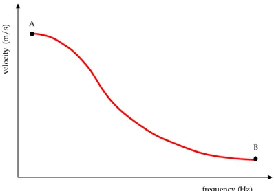
Figure 3.4 Dependence of skin depth from wavelength in a Rayleigh surface wave. To summarize the concept behind the use of the geometric dispersion for site characterization, assume that the stratified medium in Figure 3.4 is characterized by increasing stiffness with depth, so that the shear wave velocity of the top layer is less than the velocity of the second layer, which in turn is less than the velocity of the half-space below. In this situation, a high-frequency Rayleigh wave, travelling in top layer, will have a velocity of propagation slightly lower than the shear wave velocity of the first layer. On the contrary, a low-frequency wave will travel at higher velocity because it is influenced by underlying stiffer materials as well. This concept can be extended to other frequency components. A plot of phase velocity versus wavelength will hence show an increasing trend for longer wavelengths. Considering the intimate relationship between wavelength and frequency, this information can also be represented in a plot of phase velocity versus frequency (Figure 3.5), which is commonly called dispersion curve.
__________________________________________________________________________ 35 frequency (Hz) ve lo ci ty (m / s) A B
Figure 3.5 The dispersion curve describes the dispersion of surface waves: usually is depicted as phase velocity versus frequency.
The aforementioned example shows that, for vertically heterogeneous medium, the dispersion curve contains information about the variation of medium parameters with depth.
The dispersion curve can be experimentally measured and hence it is possible to interpret it in order to estimate the subsoil properties (Tokimatsu, 1995; Foti, 2000). It is a worthwhile effort to understand first which parameters actually influence the dispersion curve that can be measured.
The Rayleigh wave propagation in vertically heterogeneous media, is actually a multi-modal phenomenon: for a given stratigraphy, at each frequency different wavelength can exist. Hence different phase velocities are possible at each frequency, each of them corresponding to a mode of propagation, and the different modes can exhibit simultaneously. The different modes, except the first one, exist only above their cut-off frequency, which is for each mode the lower limit frequency at which the mode can exist: with a finite number of layers, in a finite frequency range, the number of modes is limited. At very low frequency, below the cut-off frequency of the second mode, only the first mode, known as the fundamental Rayleigh mode, exists.
Modes are not just theory or just mathematical possible solutions; they are often observed in experimental data, also in the frequency ranges of interest for a test for engineering purposes. The energy associated to the different modes depends on many factors, the stratigraphy at first, but also the depth and the kind of source.
__________________________________________________________________________ 36 The first mode is sometimes dominant in wide frequency ranges, but in many common situations higher modes play important roles and are actually dominant, and so they cannot be neglected. The different modes have different phase velocity, and so they separate at great distance from the source: otherwise they superimpose on to one another, and the mode identification can be impossible.
At the engineering scale the modal superposition is critical: the effective Rayleigh phase velocity deriving from the modal superposition is only an apparent velocity, also depending on the observation layout, on the source orientation and position.
3.4 General Setting
For the first part of this Thesis, we mainly focus on the inversion of the dispersion curves of seismic Rayleigh waves in order to obtain vertical shear stress profiles of the study area. A general scheme for this type of analysis is shown in Figure 3.6.
collected data dispersion curveExperimental
stratigraphic
model to test dispersion curvetheoretical
misfit
optimization Forward Problem
Inverse Problem
Figure 3.6 General scheme for the Thesis outline.
Surface wave methods are divided in two main categories based on the kind of sources that generate the observed signals, i.e. active and passive methods. The first ones record vibrations generated by an artificial source the frequency band of which is generally above 2 Hz (Tokimatsu, 1997). Their penetration depths are usually limited to a few tens of meters (Tokimatsu, 1997, Socco and Strobbia, 2004, Foti, 2000). On the contrary, ambient vibrations (microseisms or microtremors, if generated by nature or human activities, respectively) are produced with sources of much larger spectra, making both methods complementary for investigating deep geological structures (Wathelet et al., 2004). The determination of the
__________________________________________________________________________ 37 dispersion characteristics (dispersion curves) from passive recordings is first reviewed. Frequency wavenumber (f-k, Lacoss et al., 1969), of which conventional f-k, and high resolution frequency wavenumber (Capon, 1969) are the most popular ones.
The processing technique used in this Thesis for active experiment is a particular case of the general frequency wavenumber method. Additionally, the sensor layout deployed for the active surface wave method is the same as for refraction surveys (http://www.pasisrl.it/) and allows the measurement of Vp and Vs profiles on the first tens of meters, which brings valuable information for the inversion of the dispersion curve.
__________________________________________________________________________ 38
__________________________________________________________________________ 39
4. S
ITE
E
FFECTS
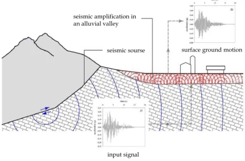
It is well known that earthquake damages strongly depend on many parameters typical of the local situation (Lanzo, 1999). Some of them concern the building vulnerability, while other ones strictly depend on the morphological configuration or shallow subsoil structure at the scale of tens to hundreds of meters; such critical phenomena are known in literature as local or site seismic effects. In particular, as an effect of the interaction between seismic input and local geomorphological/lithostratigraphical configuration, soil instabilities can be induced (soil liquefaction, landslides, etc.) or strong modification of the seismic ground motion can occur. The last effect, in particular, is responsible for most significant variations in seismic damage distribution after earthquake. Trapping of seismic waves within soft sedimentary covers overlaying a rigid bedrock (Figure 4.1) is responsible for most of this seismic amplification phenomena. Resulting resonance phenomena are able to concentrate seismic energy into a narrow frequency band (around the so called “subsoil resonance frequencies”) producing dramatic enhancement of the relevant ground motion.
seismic sourse
input signal
surface ground motion seismic amplification in
an alluvial valley
Figure 4.1 Amplification phenomena of a seismic input in shallow un-consolidated sediments overlaying a rigid bedrock (from Di Francesco, 2008, 2010).
__________________________________________________________________________ 40 The detection of seismic properties of the shallow subsoil responsible for dangerous amplification of the ground motion during earthquakes constitutes one of the basic goals for any seismic microzonation. In particular, detection of resonance phenomena requires the identification of major rigidity contrasts in the subsoil; in fact, seismic energy trapping ultimately depends on reflection/refraction phenomena that, on their turn, are mainly controlled by velocity variations of seismic phases in the shallow subsoil. Thus, defining depth distribution of P-wave and S-wave velocity (being these latter more important for potential damages), density and damping factors, is of paramount importance. Several survey techniques have been developed on purpose, that are characterized by different levels of accuracy and costs. This aspect is of great importance when extensive surveys (such as ones involved in seismic micro-zoning studies) are of concern. Due to their cost effectiveness, growing interest exists for the application of passive seismic surveys in microzonation studies and at least one international research project has been devoted to this topic (SESAME project, http://sesame.geopsy.org/). These techniques are based on the analysis of small amplitude ambient vibrations, both of natural and anthropic origin.
In the following Section a summary of all the aforementioned techniques is done; great emphasis is given to seismic noise analysis, especially single station and array analysis. A briefly description of the non-linear behavior of soils is presented, including the techniques used to evaluate them (resonance column and cyclic torsional shear tests), and liquefaction phenomenon.
4.1 Effects of Soft Surface Layers: the Amplification Function
The ground-shaking produced by an earthquake in a given site basically depends on the event magnitude, the source-to-site distance, and the local geologic conditions. When a fault ruptures below the Earth's surface, body waves travel away from the source in all directions. Since the earth's crust is not homogeneous, but it’s composed of a complex mixture of rocks and sediments of several types, as the waves reach the boundaries between different geologic materials, they are reflected and refracted. Near the ground surface, where the density and S-waves velocity are generally lower than in the materials beneath them, multiple refractions produce nearly vertical waves propagation. As mentioned before, one of the fundamental phenomenon responsible for the amplification of the motion in