ISSN: 2037-7738
GRASPA Working Papers
[online]
Web Working Papers
by
The Italian Group of Environmental Statistics
Gruppo di Ricerca per le Applicazioni della Statistica
ai Problemi Ambientali
www.graspa.org
Air quality impact assessment
of traffic policy in Milan
Alessandro Fassò
Air quality impact assessment of tra¢c policy in
Milan
Alessandro FassÚ
DIIMM - University of Bergamo
September 14, 2012
Abstract
This paper presents a general spatio-temporal model for assessing the air quality impact of environmental policies which are introduced as abrupt changes. The estimation method is based on the EM algorithm and the model allows to estimate the impact on air quality over a region and the reduction of human exposure following the considered environ-mental policy. Moreover, impact testing is proposed as a likelihood ratio test and the number of observations after intervention is computed in or-der to achieve a certain power for a minimal reduction. An extensive case study related to the introduction of the congestion charge in Milan city and the monitoring of particulate matters and total nitrogen oxides mo-tivates the methods introduced and illustrate implementation issues and inferential machinery.
1
Introduction
Environmental, energetic and industrial policies are often motivated by the need to improve air quality in terms of pollutants concentration reduction. This is usually pursued by a supposedly appropriate cut of emissive activity like selective or indistinct car tra¢c reduction, carbon energy substitution with green energy, industrial requaliÖcation, etc. Hence a fundamental step is to assess if a policy actually obtains a relevant reduction of pollutant concentrations. In this paper, we develop a general observational methodology for spatiotemporal impact assessment.
The general approach proposed is motivated by and benchmarked on a real application related to the impact of tra¢c reduction. In particular, on January 16, 2012, the Municipality of Milan introduced a new tra¢c restriction system known as congestion charge. This requires to pay a fee of Öve Euros for enter-ing the central area, known as "Area C " which is inside the so called "Cerchia dei Bastioni ". According to Municipality, in the Örst two months, car tra¢c decreased of about 36% in Area C and, at the overall city level, Municipality
reported a tra¢c reduction of about 6% which started at the beginning of Janu-ary, before the congestion charge. This bringing forward may partly be related to the preparatory campaign playd out by the administration and partly by overall decrease in gas consumption at the national level due to economic crisis. January and February have been cold and heavily polluted months with a large number of days exceeding the thresholds Öxed by the European regulations (see Arduino and FassÚ, 2012). Although the congestion charge is intended as a tra¢c control measure, the question which arise is whether there has been an impact on air quality or not. Air quality is usually deÖned according to the concentrations of various pollutants. In particular particulate matters (PM) are important because of their toxicity and are extensively monitored. Nevertheless the health e§ects of PM are known to depend not only on concentration but also on particle size, composition and black carbon content, so that having extensive data on particle numbers (see e.g. Hong-di and Wei-Zehn, 2012) or on black carbon content (see e.g. Janssen et al. 2011) would be very useful to understand air quality from health protection point of view. For other pollutants threat-ening human health, e.g. nitrogen oxides, which also are extensively monitored because of their health impact, we do not have this problem and concentration is the main health concern.
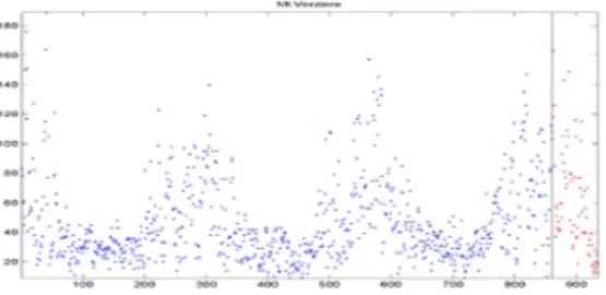
In general, comparing concentrations before and after intervention is a non-trivial problem. In fact, considering PM10 concentration in Milan city center
depicted in Figure 1, we note that the January-February mean of the last three years is 71.3 g=m3which is smaller than the after-intervention mean, obtained
between January 16 and the end of February, which is 76.7 g=m3. So the
Figure 1: PM10at Verziere Station. Black vertical line is Jan 16.
air quality impact of the tra¢c reduction due to the congestion charge has to face a major intrinsic confounder, due to atmospheric conditions, which greatly a§ects air quality in the Po Valley basin in general and Milan area in particular. Moreover a second possible confounder is related to the economic crisis which is reducing car use and gas consumption around Italy.
This paper aims at an early estimation of the spatially distributed reduction in the yearly average of pollutant concentrations. To do this, it aims to focus the following three scientiÖc questions, which are exempliÖed by means of Milan case study.
1. The Örst point is whether or not the congestion charge has a measurable permanent impact on air quality in terms of concentration reduction of particulate matters (PM10 and PM2:5) and total nitrogen oxides (NOX)
after adjusting for the e§ects of meteorological conditions and tra¢c re-duction due to economic crisis or other general áuctuations which are not related to Milan speciÖc facts.
2. Moreover, the second point aims to know if there is a di§erent impact inside the intervention area (area C) and the rest of the city.
3. Finally, the third point is related to the spatial and temporal information content required to have sound conclusions. That is the number of days, required to "observe" a statistically signiÖcant permanent impact with high probability and the number of stations required to understand the spatial impact.
In time series analysis the non spatial part of questions one and two are treated by intervention analysis after the celebrated paper of Box and Tiao (1975) : See also e.g. Hipel and McLeod (2005). Soni et al. (2004) discuss spatio-temporal intervention analysis in the context of neurological signal analysis using STARMA models. In river networks water quality monitoring, Clement et al. (2006) considered a spatiotemporal model based on directed acyclic graphs. Here, we extend these methods to a general multivariate spatiotemporal model for air quality and develop some examples related to Milan congestion charge.
With this aim, the rest of the paper is organized as follows. Section 2 presents a general spatiotemporal model, which is capable of various levels of complexity according to the information content of the underlying monitor-ing network. The estimation method is based on the EM algorithm and the model allows to estimate the impact on air quality and the reduction of hu-man exposure following the considered environmental policy. Moreover, impact testing is proposed as a likelihood ratio test and the number of observations after intervention is computed in order to achieve a certain power for a minimal reduction. In section 3, the above approach is applied to the introduction of the congestion charge in Milan city. To do this, the general model is tailored to the reduced monitoring network that the environmental agency, ARPA Lombardia, implemented for monitoring particulate matters (PM10 and PM2:5) and
nitro-gen oxides (NOX) in this city. The concentration reduction is then assessed for
the above pollutants using a preliminary vector autoregression approach and a conÖrmatory spatiotemporal model named STEM used when the spatial infor-mation contained in the monitoring network is su¢cient. The conclusions and acknowledgment sections close the paper.
2
Impact modelling by STEM
We consider here a general model able to assess the impact on air quality of an environmental rule in a geographic region R. To do this, we deÖne a spa-tiotemporal model for the observed concentration at coordinates s 2 R and day
t = 1; 2; :::; n, denoted by y (s; t), able to capture the e§ect of the environmental intervention, dated t= n m + 1 and observed for m = n t+ 1 days, namely y (s; t) = (s; t) + (t) x (s; t) + (s; t) (1) The quantity (s; t) represents the expected spatial impact of the environ-mental intervention and (s; t) = 0 for t < t: In general terms is a dynamic
random Öeld and the e§ectiveness of a environmental policy can be assessed by the expected impact on pollution concentrations over region R and time horizon M , which is given by = 1 M t+M1 X t=t Z R E ( (s; t)) p (s; t) ds
The weighting function p (s; t) may be used for averaging, e.g. p (s; t) = jRj1, or risk assessment. For example, we may be interested in human exposure and, following Finazzi et al (2012), we may take the weighting function p (s; t) as the dynamic population distribution or a time-invariant p (s) as a static population distribution over the study area. If < 0 then the impact is negative and we have an increase in pollutant concentration.
The simplest model for reduction assessment, is given by a scalar determin-istic impact
(s; t) = (2) which assumes constant impact over time and space after intervention. At an intermediate complexity level, we may use (s; t) = (s) which gives a time-invariant reduction map, appropriate for assessing a localized permanent stationary impact. Of course the choice among the above alternatives relies also on the spatial information content of the monitoring network.
Confounders may be covered by a time varying linear confounder model component (t) x (t) ; where (t) is a stationary stochastic coe¢cient vector. For example, Finazzi and FassÚ (2011b) use a Markovian dynamics for (t). In the Milan application of the next section, considering the limited amount of spatiotemporal information contained in the data, in order to avoid overÖtting and shadowing of the change point t, we use a deterministic with a minimal seasonal structure given by:
(t) =
s t 2 Summer
w t 2 W inter (3)
In equation (1), the spatiotemporal error (s; t) allows for spatial and tem-poral correlation using either separability or non-separability, see e.g. Porcu et al (2006) ; Bruno et al. (2009) and Cameletti et al. (2011). In this paper, we use a latent process with three components adapted from FassÚ and Finazzi (2011a), namely
where z (t) = z (t 1) + (t) is a stable Gaussian Markovian process, with jj < 1 and 2= V ar (). The purely spatial component ! (s; t) is given by iid
time replicates of a zero mean Gaussian spatial random Öeld characterized by a spatial covariance function given by
(js s0j) = 2!exp js s0j r (4)
with r = 1 or 2. Finally " (s; t) is a Gaussian measurement error iid over time and space, with variance 2".
2.1
Estimation and inference
We denote the parameter array characterizing model (1) by = (; ), where
is the component related solely to the e§ect () = (j) and is
the parameter component for the global dynamics of y independent on the intervention. Although, in general the impact could depend on : = (), it is convenient to deÖne models for which depends solely on . In the simple
case of equation (2), we have = / ().
With this notation, the estimated model parameter array is given by ^ =
^ ; ^
, which may be computed using maximum likelihood as in FassÚ and Finazzi (2011a) : In particular the estimates are computed using the EM algo-rithm, hence the acronym STEM for this approach. Note that the EM algorithm relies on a posteriori common latent e§ects, namely ^z (t) = E (z (t) jY ) ; which are computed by the Kalman smoother, and a posteriori local e§ects, namely ^
! (s; t) = E (! (s; t) jY ), which are computed by Gaussian conditional expec-tations. An e¢cient software for EM estimation, Öltering and kriging, called D-STEM, has been recently introduced by Finazzi (2012) and is largely used in section 3.
Using the above model, the e§ectiveness of an environmental measure may be proven by rejecting the non-change hypothesis given by
H0: () = 0
Suppose that () = 0 for = 0: We can then test the above non e§ect
hypothesis by the (one sided) likelihood ratio test. In particular, if =
is a simple scalar parameter, we can approximate the likelihood ratio test by a simple t test and reject H0for large signiÖcant values ofse( ^^). Moreover, if (s)
is a stochastic map, it may be estimated by kriging-like computations, giving the impact map ^ () and the 1 p level conÖdence bands given by
^
2.2
Days for detection and Information
Under regularity assumptions, the observed Fisher information matrix In, for
large n and m, may be related to the partitioned information i as follows
In;= m i i; i; n mi (5) where the information blocks are conformable to = (; v). It follows that
the precision in the estimation of the pollution reduction depends mainly on m.
The number of days required to detect a reduction of size with high
probability is then computed with formulas which generalize the classical sampling results. In particular for the simple scalar parametrization of (), applying the partitioned matrix inversion lemma to expression (5), we have the approximated formula m m=i1 i; m ni 1 i; 1 (1 p)1+ ()1 !2 (6)
3
Milan case study
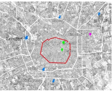
The monitoring network of Milan city, depicted in Figure 2, is composed by one station for PM2:5, four stations for PM10 and eight stations for NOX: All
these sensors give data at least three years old, that is, we consider the log-transformed and centered concentrations between January 1st, 2009, and July
20, 2012, totalling n = 1297 days and m = 186 days are after the congestion charge introduction dated January 16, 2012.
In order to adjust for the confounders, we considered meteorological condi-tions in Milan, namely wind speed (daily maximum and average) and direction, humidity, temperature, solar radiation and pressure. Moreover, we used the additional covariates given by the concentration readings of the same pollutants in Bergamo city which is approximately 45km North-East of Milan and we used data from the urban ground station known as Meucci. This is an important proxy for all other meteorological and economic factors common to the north plain of Lombardy but the congestion charge in Milan.
3.1
Modelling details
Due to the sparsity of Milan data, we start using three di§erent simple ex-ploratory q-dimensional vector seasonal autoregressive (ARX) models. For PM2:5 we use only a unidimensional ARX model, while for PM10 and NOX,
we integrate the analysis of the vector ARX models with the STEM approach of the previous section.
The exploratory ARX models are given by yt= at+ bxt+ Gyt1+ et
Figure 2: Milan Area C (red line) and monitoring network.
Blue pushpins: NOX only, from top right counterclockwise Lambro, Marche,
Zavattari, Liguria, Abbiategrasso.
Green Ballons: PM10 and NOX, Area C, Senato and Verziere.
where yt is PM2:5, PM10 or NOX with dimensions q = 1; 3 and 7, respectively.
The impact at is as in equation (2) and, similarly, the seasonal adjustment b
is as in equation (3). The covariates are selected by taking into account BIC criterion and residual autocorrelation. The persistence matrix G is taken as a diagonal matrix:
G = diag (g1; :::; gq)
Note that the multivariate approach is important here, because the errors et
may be strongly (spatially) correlated.
According to the AR(1) dynamics, the scalar steady state impact on yt is
given by
d = a
1 g (7)
Moreover, ignoring the uncertainty of the pre-intervention estimation of g and recalling the Fisher information matrix given in (5), we get the approximate variance for ^d; namely
V ard^= V ar (^a) = (1 ^g)2 It follows that the city average steady state e§ect is given by
d = qj=1d^jpj
with variance given by the well known quadratic form: V ard= p0V arD^p
In the above formula, D = (d1; :::; dq) and the weights p = (p1; :::; pq) can be
based on the population density, which is taken as approximately constant in the rest of the paper, as we are involved in city center data especially for the PM study.
3.2
Fine particulate matters
We start with the single station on Öne particulate matters PM2:5, namely
Pas-cal station, which is a ground station external to "Area C" and located in the relatively central quarter named "Citt‡ studi". Here, Öne particulate concentra-tions have a three-year average of approximately 30g=m3 before intervention.
After January 16 the January-February three year mean increased from 53.7 g=m3 to 54.1 g=m3, questioning the congestion charge e§ect.
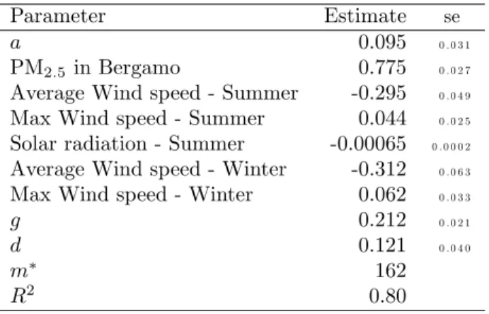
To Öt the model for Öne particulate matters, we use the centered log trans-formed concentrations which have variance 2
y = 0:70, and, after row deletion
of missing data, we get the Ötted model of Table 1 based on the remaining 1038 observations. It is worth noting that wind speed has an e§ect both in summer and winter while, not surprisingly, solar radiation is not signiÖcant in winter. After adjusting for Bergamo concentrations which are quite signiÖcant in the model, the residual autocorrelation is not large resulting in g = 0:212.
Parameter Estimate se
a 0.095 0 . 0 3 1
PM2:5 in Bergamo 0.775 0 . 0 2 7
Average Wind speed - Summer -0.295 0 . 0 4 9
Max Wind speed - Summer 0.044 0 . 0 2 5
Solar radiation - Summer -0.00065 0 . 0 0 0 2
Average Wind speed - Winter -0.312 0 . 0 6 3
Max Wind speed - Winter 0.062 0 . 0 3 3
g 0.212 0 . 0 2 1
d 0.121 0 . 0 4 0
m 162
R2 0.80
Table 1: ARX model and reduction for PM2:5
Since we are in log scale, the permanent e§ect, computed as both ^a or ^d of equation (7), may be interpreted as a percent change. According to this model, at Pascal station, we observe a 0:12 permanent reduction of PM2:5 on log scale
with a one-sided p-value smaller than 0:2%. From the bottom row of Table 1, we see that Ötting is quite good. The residuals result to be satisfactorily white noise but moderately non Gaussian as shown by Figure 3 and by unreported kurtosis which are larger than three. Although some alternatives to conditional Gaussian models could be developed, see e.g. Bartoletti and LoperÖdo (2010) or Nadarajah (2008), the above results where validated by simulation experiments and by comparison with robust estimation methods getting very close results to Table 1.
Figure 3: Residuals of PM2:5 at Pascal station.
Days for detection From the practical point of view it is important to see which is the number of days required to detect a certain reduction in the annual average of PM2:5: Following the approach which gives formula (6), we
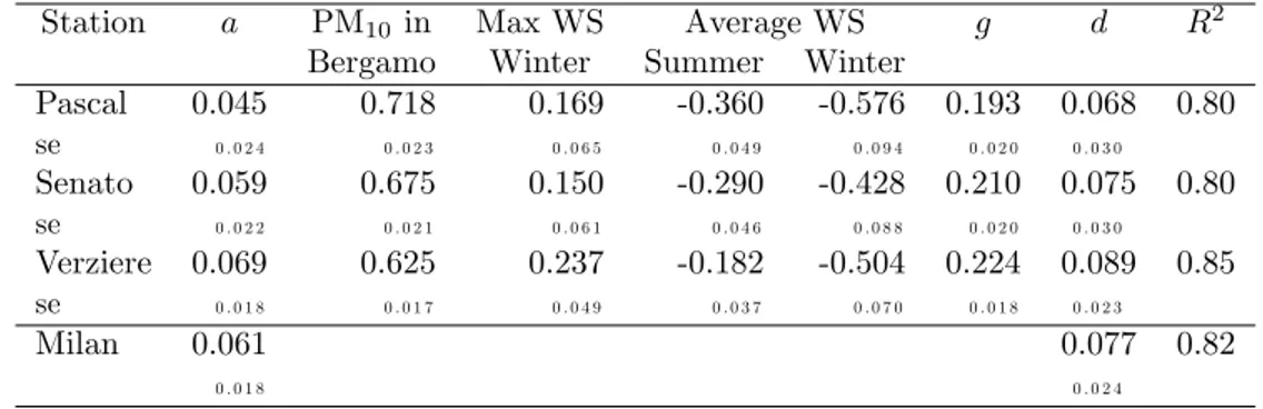
Station a PM10in Max WS Average WS g d R2
Bergamo Winter Summer Winter
Pascal 0.045 0.718 0.169 -0.360 -0.576 0.193 0.068 0.80 se 0 . 0 2 4 0 . 0 2 3 0 . 0 6 5 0 . 0 4 9 0 . 0 9 4 0 . 0 2 0 0 . 0 3 0 Senato 0.059 0.675 0.150 -0.290 -0.428 0.210 0.075 0.80 se 0 . 0 2 2 0 . 0 2 1 0 . 0 6 1 0 . 0 4 6 0 . 0 8 8 0 . 0 2 0 0 . 0 3 0 Verziere 0.069 0.625 0.237 -0.182 -0.504 0.224 0.089 0.85 se 0 . 0 1 8 0 . 0 1 7 0 . 0 4 9 0 . 0 3 7 0 . 0 7 0 0 . 0 1 8 0 . 0 2 3 Milan 0.061 0.077 0.82 0 . 0 1 8 0 . 0 2 4
Table 2: Vector ARX model and reduction for PM10, Single stations and city
average. WS stands for Wind speed.
consider the t-test for the hypothesis of no impact H0: d = 0 against a reduction
d > 0 based on large values of the statistic se(^^aa): Using the nominal signiÖcance level p = 5%, the number of days for detecting a permanent reduction of size d = 0:10 in log scale with probability = 85% is given by m m= 162 as
shown in Table 1, which is consistent with the above results.
3.3
Particulate matters
For the PM10; we have three sites, two are tra¢c stations located inside "Area
C", namely Verziere and Senato stations, and the third is Pascal, which is a ground station located in Citt‡ studi which is semi-peripheral area with patterns similar to the city center.
Table 2 shows the Ötted model for PM10. We see that the persistence
coef-Öcients g are small and very close each other, denoting the same weak autocor-relation after adjusting for the Po valley concentration proxy given by Bergamo measurement and local meteorological covariates. Both average and maximum wind speed have an e§ect on PM10 with a clear seasonal behaviour. The last
column shows that Ötting is quite satisfactory. We note that, after introducing the Bergamo proxy, only local conditions given by wind speed enter as additional covariates.
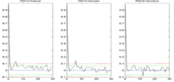
As in the previous section, a moderate residual non normality indicated by kurtosis larger than three for all components does not jeopardize the results of Table 2. Moreover, Figure ?? shows that the residuals can be assumed to be a white noise and the importance of the multivariate approach is appreciated by the marked residual correlation shown in Table 3.
Note that the global three-year average for these stations before intervention is about 45g=m3, so the average reduction of d = 0:137 in log scale, with se =
0:053, corresponds approximately to 6g=m3for the yearly average. According
Citt‡ studi 1 0.65 0.58 Senato 1 0.69
Verziere 1
Table 3: ARX model residual correlations for PM10
Figure 4: Residual autocorrelations of Vector ARX model for PM10.
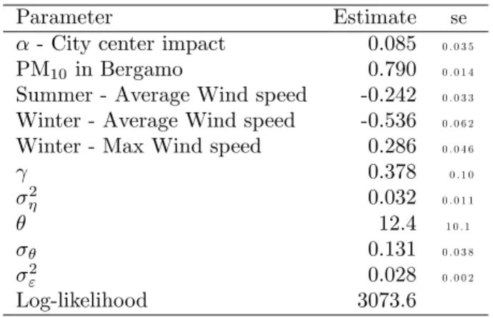
STEM approach In the light of the preliminary analysis, we go further with the approach of section 2, obtaining the Ötted model of Table 4. To avoid initial values dependence, the EM algorithm has been replicated 100 times ap-plying beta distributed random perturbations1 to the initial estimates which
have been computed using the method of moments. The power r of the spa-tial correlation (4) has been selected to r = 1 comparing the corresponding log-likelihoods.
Generally speaking the standard errors are small, with the exception of the spatial correlation parameter ; which has a quite large uncertainty. This is not surprising since with only three stations is not easy to estimate spatial correla-tion. The reduction parameter is positive, denoting a signiÖcant permanent reduction of particulate concentrations of 0:085 in log scale for the city center with one sided p-value smaller than 1%.
Moreover, the likelihood ratio test for the hypothesis of no e§ect, namely H0 : = 0; gives a test statistic 2log (LR) = 13:2 with a p-value smaller than
0:1%. Finally, the number of days for detection of formula (6), with nominal signiÖcance level p = 5%, a permanent reduction of size = 10% and power
= 85% results to be m= 154 which is consistent with above results.
According to ARX model, Area C has a little larger PM10 reduction, but
the di§erence in a coe¢cients of Table 2 is far from signiÖcant. Using STEM model, the corresponding analysis is based on the a posteriori local e§ects of section 2.1, that is ! (s) = m1 Pnt=t! (s; t) which are smaller than 1% and have^
non signiÖcant p-values for Pascal, Senato and Verziere. Hence we can conclude the reduction in PM10 is approximately constant around the city center but we
1At each replication, the initial values have been rescaled between 0 and three times their
value by multiplication with random numbers 3B where B0shave been drawn from the Beta
Parameter Estimate se
- City center impact 0.085 0 . 0 3 5
PM10in Bergamo 0.790 0 . 0 1 4
Summer - Average Wind speed -0.242 0 . 0 3 3
Winter - Average Wind speed -0.536 0 . 0 6 2
Winter - Max Wind speed 0.286 0 . 0 4 6
0.378 0 . 1 0 2 0.032 0 . 0 1 1 12.4 1 0 . 1 0.131 0 . 0 3 8 2 " 0.028 0 . 0 0 2 Log-likelihood 3073.6 Table 4: STEM model for PM10
have no information on peripheral areas.
3.4
Nitrogen oxides
As mentioned above, the total nitrogen oxides are monitored in Milan city more extensively than particulate matters. In fact, in addition to the previous three stations, we have four tra¢c stations near the internal bypass and one ground station in the green area of Parco Lambro, near the eastern circular highway and exposed to Linate airport emissions. Using this relatively larger network, we will address the spatial variability of the congestion charge impact around the city. We Örst observe that nitrogen oxides data are given as hourly data. In order to have high quality daily data, and considering that STEM approach is resistant to missing data, we deÖned as missing those daily averages based on less then 20 validated observations. An additional meteorological covariate enters at this stage which was not signiÖcant with particulate matters. This is the prevalence of South western wind (SW-PWD) deÖned as the number of hours per day when the prevailing wind is from SW.
The vector ARX model for these eight stations is reported in Table 5. We keep this as a preliminary analysis model even if, with such a number of spatial locations, a vector approach begins showing its limitations and the need for a uniÖed approach such as STEM is now becoming evident. The proxy from Bergamo and the seasonal e§ect on wind are again decisive for the good model Ötting, reported in the last column of Table 5. As mentioned above, the wind direction from South West is signiÖcant for various stations. Despite the number of monitoring stations, the impact of the congestion charge on NOX is far from
constant around the city.
In Pascal station, we have the maximum reduction, more than 0:28 in log scale and p-value close to zero. Surprisingly this value is much larger than inside the tra¢c restricted Area C, where the permanent e§ect estimated by the ARX
model is positive but very small especially in Verziere. Moreover, in peripheral stations, at Liguria and Lambro stations, we have signiÖcant increases in NOX
concentrations. Note that this fact is not a model artifact but reáects the daily averages behaviour. These points will be partially overcome in the Önal STEM model.
Statio n a Su mmer Win ter N OX in gR 2 Av e W S M a x W S SW -P WD A v e WS Max WS Berga m o P a scal 0 .295 -1.004 0. 401 -0.00 17 -1. 20 0.487 0. 539 -0. 328 0.8 5 se 0.03 0 .12 0. 09 0 .003 0.13 0.10 0. 03 0.02 Se nato 0 .046 -0.303 0. 107 -0.00 77 -0.6 18 0.335 0. 396 -0. 420 0.8 7 se 0 .025 0. 094 0. 072 0 .0026 0.11 0.084 0. 024 0.025 V er zi er e -0.006 4 -0.669 0. 323 -0.00 95 -0.8 39 0.376 0. 489 -0. 260 0.8 3 se 0 .025 0. 097 0. 074 0 .003 0.11 0.087 0. 025 0.025 Lig u ria -0.13 6 -0.760 0. 390 -0.02 2 -0.7 79 0.345 0. 307 -0. 360 0.7 9 se 0.02 0. 091 0. 069 0 .003 0.10 0.081 0. 02 0.02 Marc h e 0 .018 -0.75 0. 228 -0.02 3 -0. 96 0.33 0. 340 -0. 256 0.8 3 se 0.02 0 .09 0. 06 0 .002 0.10 0.08 0. 02 0.02 Abb iategrasso -0.05 4 -0.807 0. 288 -0.00 11 -1. 18 0.630 0. 400 -0. 368 0.8 5 se 0.03 0 .11 0. 08 0 .003 0.12 0.097 0. 027 0.025 Lam bro -0.11 5 -0.736 0. 288 -0.00 54 -1. 17 0.552 0. 374 -0. 365 0.8 1 se 0.03 0 .10 0. 08 0 .0029 0.12 0.093 0. 026 0.025 Za v atta ri -0.01 3 -0.701 0. 214 0 .017 -0. 98 0.470 0. 454 -0. 239 0.8 3 se 0.03 0. 087 0. 07 0 .002 0.099 0.078 0. 023 0.024 T able 5: V ector A RX m o d el for NO X . W S st an ds for Wind Sp eed , S W-PWD for S outh w este rn prev ail ing wi n d d irec tion.
The residuals of this model are satisfactorily Gaussian, white noise and ho-moskedastic according to standard tests. Note that the estimated permanent reduction for Pascal is quite large, ^d = 0:44 with a standard error se = 0:05; and will be discussed in the next section.
STEM approach In order to deepen the urban variability and seek for a uniÖed conclusion about the congestion charge impact on nitrogen oxides concentrations, we consider a STEM model with spatially varying impact. In the light of the limited spatial information contained in Milan eight station network, we use the following simple impact model for t t
(s) =
1 s 2 City center
2 s =2 City center
(8)
where, for the purpose of this paper, the city center is deÖned by Area C plus Citt‡ studi, as discussed in the previous section. The estimated model, reported in Table 6, clearly shows the di§erence between the impact in the city center, where a permanent reduction of about 0:23 in log scale is estimated, and the peripheral area where NOX concentrations show an increase of 0:07, although
not statistically signiÖcant. To have a conÖrmation about the non-increase in the peripheral area, we tested the hypothesis 2 = 0 using the Likelihood
ra-tio test. This approach gives a restricted Log-likelihood of 6515:0 and a non signiÖcant LR statistic with p-value = 15:7%. Interestingly the spatial correla-tion parameter is very close to the PM10 case but, as expected, the standard
deviation is smaller reáecting the major spatial information of nitrogen oxides network.
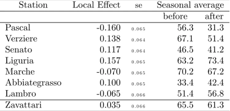
The local e§ects ! (s) of section 2.1 are reported in Table 7. Note that, considering for example Pascal, if we sum up 1 from Table 6 and ! (s) from
Table 7 we get a total reduction of 0:402 which is quite close to the estimate ^d of the ARX model. Note that these results reáect the change in the unadjusted seasonal average concentration. For example in the last two columns of Table 7, we have the comparison of the average concentrations in the period January 16 - July 20 before and after the congestion charge introduction, in the years 2009-2011 and 2012 respectively.
4
Conclusions
In order to answer the three scientiÖc questions on air quality impact raised in the introduction, we introduced a general approach, based on STEM model, for spatiotemporal impact assessment of air quality policies allowing both estima-tion and testing.
The Örst question on the presence of a "permanent impact" is positive. In particular, we showed that the congestion charge operating in Milan center since January 16, 2012, has a signiÖcant permanent impact on air quality in terms
Parameter Estimate s e Central impact - 1 0.218 0 . 0 4 8 Peripheral impact - 2 -0.077 0 . 0 4 7 Summer Average WS -0.706 0 . 0 5 4 Max WS 0.267 0 . 0 4 2 South West -0.0073 0 . 0 0 1 4 Winter Average WS -1.021 0 . 0 6 1 Max WS 0.552 0 . 0 5 0 BG.NOX 0.604 0 . 0 1 6 0.599 0 . 0 4 8 2 0.033 0 . 0 0 4 7 12.7 3 . 7 0.153 0 . 0 1 3 2 " 0.054 0 . 0 0 2 Log-likelihood 6516.0
Table 6: STEM model for NOX. WS stands for Wind speed.
Station Local E§ect se Seasonal average before after Pascal -0.160 0 . 0 6 5 56.3 31.3 Verziere 0.138 0 . 0 6 4 67.1 51.4 Senato 0.117 0 . 0 6 4 46.5 41.2 Liguria 0.157 0 . 0 6 5 63.2 73.4 Marche -0.070 0 . 0 6 5 70.2 67.2 Abbiategrasso 0.100 0 . 0 6 5 33.4 42.4 Lambro -0.065 0 . 0 6 6 51.4 56.8 Zavattari 0.035 0 . 0 6 6 65.5 61.3
Table 7: STEM local e§ects ! (s) for NOX, in log scale, and unadjusted seasonal
of particulate matters and nitrogen oxides concentrations at least in the city center. The air quality impact has been estimated after adjusting for meteoro-logical factors and other common forcing factors, such as the economic crisis. Interestingly, the reduction on PM2:5, PM10and NOX concentrations estimated
using both a preliminary vector autoregressive model and STEM approach, is not conÖned inside the tra¢c restricted area.
The second question, on the spatial distribution of the air quality change has an articulated answer. We observed that, despite the reduced number of monitoring stations in the city, the impact has a noticeable spatial variability which is di§erent for PM10and NOX. In particular, after the tra¢c intervention,
a signiÖcant reduction of both particulate matters and nitrogen oxides has been estimated in the city center. The reduction of particulate matters, which is about 8%, or 3:6 g=m3, in city center, is slightly higher in the intervention
area, but the spatial variations around the city center either inside or outside the Area C can be neglected. The nitrogen oxides show di§erent Ögures and pattern, with a reduction larger than 19%, or 13 ppb, in city center. Surprisingly, the reduction is higher in Citt‡ studi, outside the intervention area, while in Verziere, which is inside Area C, the reduction is barely signiÖcant. Moreover, in the peripheral areas of the city, we observe changes of nitrogen oxides in both directions and no overall decrease can be concluded.
Considering the third question on spatiotemporal information, we observe that, using the data before August 2012 gives a substantially clear picture of air quality impact, at least in the city center. Nevertheless, having a more ex-tended monitoring network, would allow us to estimate more detailed reduction maps both for pollutant concentrations and human exposure by means of the dynamical kriging capabilities of the STEM approach proposed in this paper.
5
Acknowledgments
This research is part of Project EN17, ëMethods for the integration of di§erent renewable energy sources and impact monitoring with satellite dataí, Lombardy Region under ëFrame Agreement 2009í.
The help of Angela Locatelli and Francesco Miazzo for data handling has been much appreciated by the author.
References
[1] Arduino G., FassÚ A., (2012) Environmental regulation in the European Union. In Abdel H. El-Shaarawi and Walter W. Piegorsch (eds) Encyclo-pedia of Environmetrics 2nd ed., Wiley. In printing.
[2] Bartoletti S., LoperÖdo N. (2010) Modelling air pollution data by the skew-normal distribution. Stochastic Environmental Research and Risk Assess-ment. 24:513ñ517.
[3] Box G. E. P. and Tiao G. C. (1975) Intervention Analysis with Applications to Economic and Environmental Problems. Journal of American Statistical Association. 70(349):70-79.
[4] Bruno F., Guttorp P., Sampson P.D., Cocchi D. (2009) A simple non-separable, non-stationary spatiotemporal model for ozone. Environ Ecol Stat.16:515ñ529.
[5] Cameletti M. Ignaccolo R. Bande S. (2011) Comparing spatio-temporal models for particulate matter in Piemonte, Environmetrics. 22(8):985ñ996 [6] Clement L., Thas O., Vanrolleghem P.A. and Ottoy J.P. (2006) : Spatio-temporal statistical models for river monitoring networks. Water Science & Technology. 53(1):9ñ15.
[7] FassÚ A, Finazzi F, (2011a) Maximum likelihood estimation of the dynamic coregionalization model with heterotopic data. Environmetrics. 22(6):735-748.
[8] Finazzi F. (2012) D-STEM ñ A statistical software for multivariate space-time environmental data modeling. METMA VI International Workshop on spatio-temporal modelling. Guimaraes, 12-14 September 2012. In printing. [9] F. Finazzi, A. FassÚ (2011b). Spatio temporal models with varying coe¢-cients. In Cafarelli Ed. (2011) Spatial Data Methods for Environmental and Ecological Processes ñ 2nd Edition, Foggia, Sept. 1-2, 2011. ISBN: 978-88-96025-12-3. Also in: Graspa WP, 2011, www.graspa.org, ISSN: 2037-7738. [10] Finazzi F., Scott M.E. , FassÚ A. (2012). A statistical framework for model based air quality indicators and population risk evaluation. GRASPA WP, 43:1-26. www.graspa.org, ISSN: 2037-7738.
[11] Graf-Jaccottet M, Jaunin MH. (1998) Predictive models for ground ozone and nitrogen dioxide time series. Environmetrics. 9:393ñ406.
[12] Hipel, K.W. & McLeod, A.I. (2005) Time Series Modelling of Water Re-sources and Environmental Systems. c 2005 Hipel, K.W. & McLeod, A.I.. http://www.stats.uwo.ca/faculty/aim/1994Book/
[13] Hong-di H., Wei-Zhen L. (2012) Urban aerosol particulates on Hong Kong roadsides: size distribution and concentration levels with time. Stochastic Environmental Research and Risk Assessment. 26:177ñ187.
[14] Janssen N.A., Hoek G., Simic-Lawson M., Fischer P., van Bree L., ten Brink H., Keuken M., Atkinson R.W., Anderson H.R., Brunekreef B., Cassee F.R. (2011) Black Carbon as an Additional Indicator of the Adverse Health Ef-fects of Airborne Particles Compared with PM10 and PM2.5. Environmen-tal Health Perspectives. 119:1691-1699.
[15] Nadarajah S (2008) A truncated inverted beta distribution with application to air pollution data. Stochastic Environmental Research and Risk Assess-ment. 22:285ñ289.
[16] Porcu E., Gregori P., J Mateu J. (2006) Nonseparable stationary anisotropic spaceñtime covariance functions. Stochastic Environmental Re-search and Risk Assessment. 21:113-122
[17] Soni P, Chan Y, Preissl H, Eswaran H, Wilson J, Murphy P, Lowery CL (2004) Spatial-Temporal Analysis of Non-stationary fMEG Data. Neurology and Clinical Neurophysiology. 100:1-6.