DOTTORATO DI RICERCA
Ciclo XXI Settore FIS/07
Monte Carlo Simulations of Novel Scintillator Detectors and
Dosimetry Calculations
Dr. Sergio Lo Meo
Coordinatore Dottorato: Relatore:
Chiar.mo Prof. F. Ortolani Chiar.mo Prof. F. L. Navarria
In primis, il Prof. F. L. Navarria per l’opportunit´a che mi ha dato e per tutto cio’ che mi ha insegnato.
Il Dr. Andrea Perrotta, “il piu’ grande esperto di geometrie 3D presente nell’universo e in quelli ipotizzati”, per le sue dritte illuminanti nei momenti piu’ critici.
Il Dr. Nico Lanconelli, per il continuo e fondamentale aiuto.
Il Prof. R. Pani, per il prezioso supporto teorico e sperimentale necessario allo svolgimento di questo lavoro di tesi.
La Dr.ssa R. Pellegrini, la Dr.ssa M. N. Cinti ed in particolare ll Dr. P. Bennati, sempre presente, in qualsiasi ora del giorno e della notte, per fornirmi i dati necessari alle mie simulazioni.
Oltre ai doverosi “acknowledgments” professionali, ci tengo a ringraziare varie persone per la loro vicinanza affettiva.
Mia moglie Mariya per l’amore e la pazienza di questi anni.
Mia figlia Sasha, per la dolcezza e la gioia che mi trasmette nei momenti di maggior stanchezza.
Contents
Introduction 1 1 SCINTIRAD 3 1.1 Introdution . . . 3 1.2 Biological studies . . . 4 1.2.1 Rhenium-188 . . . 5 1.2.2 Studies in “vitro” . . . 6 1.2.3 Studies in “vivo” . . . 10 1.3 GEANT4 overview . . . 13 1.4 Dose calculation . . . 17 1.4.1 Simulation setup . . . 17 1.4.2 Cross checks . . . 19 1.4.3 Results . . . 24 1.5 Experimental biodistribution . . . 251.5.1 Energy resolution of the YAP camera . . . 27
1.5.2 Spatial resolution of the YAP camera . . . 28
i
1.5.3 First measurements with 188Re . . . . 30
2 Lanthanum Bromide Crystals 33 2.1 Introduction . . . 33
2.2 Lanthanum Bromide features . . . 34
2.3 Experimental setup . . . 36
2.4 Photodetection principle . . . 38
2.4.1 Linearity and Spatial Resolution . . . 41
2.4.2 Energy Resolution . . . 43
2.5 Simulation setup . . . 44
2.6 Results . . . 49
3 ECORAD 63 3.1 Introduction . . . 63
3.2 Ultrasound probe design . . . 64
3.3 Scintigraphic camera . . . 66 3.3.1 Slant collimator . . . 66 3.3.2 Simulation setup . . . 69 3.4 Experimental setup . . . 72 3.5 Simulation results . . . 73 Conclusions 79 A GEANT4 Optical Physics 83 A.1 Optical photons . . . 83
A.2 Scintillation process . . . 84
A.3 Tracking optical photons . . . 85
A.3.1 Absorption . . . 85
A.3.2 Rayleigh scattering . . . 86
A.3.3 Boundary process . . . 87
B Acronyms 95
Introduction
Monte Carlo (MC) simulation techniques are becoming very common in the Medical Physicists community. Various general purpose MC codes, initially developed to simu-late particle transport in a broad context, can be used also for modeling Single Photon Emission Computed Tomography (SPECT) and Positron Emission Tomography (PET) configurations [1]. As they have been designed for a large community of researchers, these codes are well documented and are available in the public domain. Several topics are addressed by MC in the Nuclear Medicine (NM) field, among them, in this study, we present the use of MC for optimization of SPECT imaging systems design and for dosimetry calculations.
Radiation plays a key role in the treatment of many cancer types and in medical diagnosis. Radiotherapy with radiation other than gamma and X-rays has become important based on the specific physical properties of alpha and beta-emitting ra-dionuclides. A Technetium congener, Rhenium-188 (188Re), is a promising candidate
for radiotherapeutic production. In the first Chapter, we present results obtained on the radio-response of 188Re-perrhenate in a panel of human tumor cell lines.
Inhibi-tion of cell proliferaInhibi-tion, inducInhibi-tion of micronuclei and apoptosis have been considered as measures to ascertain the sensitivity of the tumor cell to the β-emission of 188Re.
The dosimetry of 188Re, used to target the different lines of cancer cells, has been
evaluated by the MC code GEANT4 [2]. The simulations estimate the average energy
deposition/per event in the biological samples.
While the 188Re beta emission is fundamental for therapeutic purposes [3], the
gamma rays can be detected, by gamma-cameras, to evaluate the biodistribution of the radionuclide and for a real-time SPECT monitoring of regional drug concentration during radiation therapy. With the use of 188Re for imaging purposes in mind, in the
second Chapter we present a study of gamma-cameras based on planar scintillation crystals of Lanthanum Bromide doped with Cerium (LaBr3:Ce). The simulation tests,
by GEANT4, start from a radioactive decay source and halt when the scintillation photons reach the photomultiplier (PM). In the simulations, the boundary processes on all crystal surfaces are considered. Different LaBr3:Ce crystal configurations are
simulated in view of optimizing the gamma-camera performance.
The visual quality and quantitative accuracy of radionuclide imaging, however, of-ten lacks anatomic cues that are needed to localize or stage the disease and typically has poorer statistical and spatial characteristics than anatomic imaging methods, such as an ultrasound system. These issues have motivated the development of a new ap-proach that combines functional data from compact gamma cameras with structural data from ultrasound equipments. The aim is to develop a dual integrated portable camera able to acquire tomographic images obtained by using simultaneously ultra-sound and scintigraphic techniques. In the third Chapter preliminary results obtained for the setup of the ECORAD collaboration are described, and some simulated results of the scintigraphic part of the system are shown.
Chapter 1
SCINTIRAD
1.1
Introdution
SCINTIRAD [4] is a multidisciplinary collaboration that aims at determining the ra-dioresponse of188Re, a β−and γ emitter used in metabolic radiotherapy. The response
with cells “in vitro”, the biodistribution in different organs of mice “in vivo”, and the therapeutic effect on liver and other tumors induced in mice, have been studied. SCINTIRAD is based on a large scientific collaboration:
• The National Institute of Nuclear Physics (INFN) sections of Bologna, Roma 1, Roma 3 and Legnaro.
• Physics Dept. - Alma Mater Studiorum - University of Bologna. • Experimental Medicine Dept. “Sapienza” University of Rome. • Physics Dept., Biology Dept. - University of Rome 3.
• Physics Dept., Pharmacology Science Dept., Pathology and Veterinary Hygiene Dept., Oncology and Surgical Sciences Dept. - University of Padua.
• Natural Sciences Dept. - Shumen University (Bulgaria).
• Dept. of Technology and Health - Italian Istitute of Health (ISS).
188Re is a promising candidate for application in NM [5]. While the beta emission is
fundamental for therapeutic purposes, the gamma rays can be detected to evaluate the biodistribution of the radionuclide and for a real-time SPECT monitoring of regional drug concentration during radiation therapy. Hyaluronic Acid (HA) is a molecule al-ready adopted as a suitable vector of chemotherapeutic drugs [6]. Technetium-99m HA (99mTc-HA) labeling procedure and biodistribution studies have been previously
reported in literature [7]. HA has also been adopted as a vector for 188Re and
prelimi-nary results on the effect of a 188Re-perrhenate solution on a series of tumor cell lines
obtained in vitro have been presented in [8].
The dosimetry of 188Re used to target the different lines of cancer cells has been
evaluated by a MC simulation based on GEANT4, and the preliminary results obtained are presented in Section 1.4.
1.2
Biological studies
Radiotherapy with radiation other than gamma and X-rays has become important based on the specific physical properties of alpha and beta-emitter radionuclides when conjugated with biologic molecules carrier, such HA, monoclonal antibodies, etc. As a result of tumor targeting, a cell-focused delivery of radiation is obtained compared to irradiation with sparsely ionizing gamma or X-rays, leading furthermore to the advantage of treating widely disseminated diseases as secondary or metastasis cancer. A major factor in the failure of radiotherapy is represented by inherent or induced cellular radioresistance [9]. In fact, it is well established that different human tumor
types can differ greatly in their sensitivity to radiation [10]. Up to now, the intrinsic radiosensitivity has been evaluated in a large panel of human tumor cell lines after “in vitro” exposure to gamma or X-rays. Conversely, scanty data are available in the literature on the radioresponse of tumor cells after treatment with radiopharmaceuticals characterized by beta-emission. To gain this piece of information is particularly relevant considering that the radiosensitivity “in vitro” can predict the outcome of irradiation “in vivo”.
Molecular mechanisms in which cell death is caused by beta-irradiation are not well understood and no data on beta-irradiation-induced apoptosis of cells derived from solid tumors are available in the literature. 188Re, is a promising candidate for
radiotherapeutic production and understanding the mechanisms of the radioresponse of tumor cells to 188Re is of crucial importance as a first step before “in vivo” studies,
where the same cells may be inoculated/injected in mice and then treated with a biomolecule conjugated with 188Re. In this respect, since in most malignant cell types
the specific membrane receptor CD44 is typically overexpressed [11], HA, which binds CD44, can be successfully exploited as 188Re carrier.
1.2.1
Rhenium-188
Rhenium is a chemical element with the symbol “Re” and atomic number 75. Rhenium (Latin Rhenus meaning “Rhine”) is the next-to-last naturally occurring element to be discovered and the last element having a stable isotope. Its isotope, 188Re, has
chemical properties similar to the widely used congener 99mTc, this permits to use all
the information on the biodistribution of99mTc-radiopharmaceutical to be used for the
research of effective 188Re-radiotherapeuticals.
188Re decays [12] to188Os (70%) or188Os∗ (30%) with a half-life of about 17 hours,
energy of 2.12 MeV (0.78 MeV average energy). At the maximum energy, the electron is absorbed within a radius of 11 mm in biological tissues. In addition, 188Os∗ emits
promptly (0.69 ns) a γ-ray, mainly in the line at 155 keV but with the photon spectrum extending up to about 2 MeV. In 15.6 % of the 188Re decay chains, a 155 keV photon
is emitted.
1.2.2
Studies in “vitro”
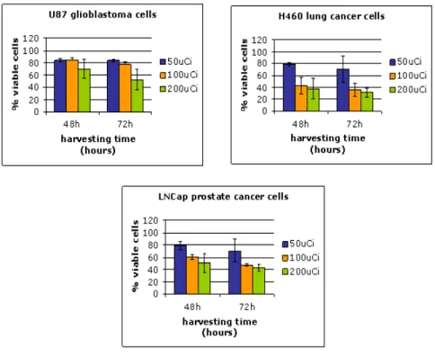
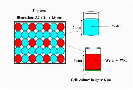
Cells were seeded at appropriate concentrations in 96-multiwells (4 wells/cell line; 100 µl/well) [8]. Cell cultures are deposited inside the (darkest) wells of the experimental setup, as shown in Fig. 1.1.
Figure 1.1: A picture of the wells used to assess biological response to 188Re of a set of
human tumor cell lines. The rectangle indicates the well geometry used in the MC simulation (see Section 1.4).
Active wells are interleaved by empty holes filled with water, acting as absorbing medium, to simplify the evaluation of the dose. Neoplastic cells of different histotypes (H460 lung cancer cells, U87 glioblastoma, LnCaP prostate tumor cells) are used. The data (Fig. 1.2 ) are presented as percentages of viable cells, in cultures188Re-exposed,
with respect to untreated ones.
Figure 1.2: Percentages of viable cells in tumor cell lines exposed for 48 or 72 h to188
Re-perrhenate.
After 48 or 72 h, by using specific initial activities ranging from 18.5 to 74 GBq/l, the evaluation is done by means of a recognized test for cytotoxicity which measures mitochondrial metabolism in the entire cell culture: MTT1assay [16]. Inhibition of cell
proliferation, induction of micronuclei and apoptosis have been considered as measures
to ascertain the sensitivity to the β-emission of 188Re. 188Re-perrhenate treatment
clearly indicates that the different tumor cells tested show different sensitivities. Ra-dioresistance is characteristic of many different tumor types, among them glioblastomas are considered particularly radioresistant and long-term survivors with this diagnosis are very rare [17].
U87 glioblastoma cells showed about 20% reduction in cell viability (compared to untreated cultures, as shown in Fig.1.2) at both 48 and 72 h harvesting times. The maximum cellgrowth inhibition leading to 45% reduction of the cell viability is obtained after 72 h radiation exposure with initial specific activity of 74 GBq/l. On the contrary, both H460 and LnCap show a higher sensitivity to beta emissions of188Re and this is
particularly visible at 72 h harvesting time.
As a next step, the relationship between cell death assessed by the MTT assay and the induction of apoptosis, a process that removes highly damaged cells from the replicative pool to maintain genome integrity, is checked. Cells are fixed, ei-ther in absolute methanol for 30 min and stained with 2.5 mg/ml DAPI2 or in 4%
paraphormaldeide and processed for the TUNEL3 assay [18], in which the terminal
deoxynucleotidyl transferase binds to 3’-OH ends of DeoxyriboNucleic Acid (DNA) fragments generated in response to apoptotic signals and catalyses the addition of biotin-FITC-labeled deoxynucleotydes4. Then the cells are exposed 48 h to 74 GBq/l 188Re-perrhenate and the results show that U87 (Fig. 1.3) are extremely resistant to
the induction of apoptosis. On the contrary for H460 and LnCap cells. In the graph of the Fig. 1.3 are reported the frequency of apoptotic cells induced after treatment (t − test: * P < 0.05; ** P < 0.01).
24’-6-Diamidino-2-phenylindole (DAPI) is known to form fluorescent complexes with natural
double-stranded DNA, showing a fluorescence specificity for AT, AU and IC clusters.
3Terminal deoxynucleotidyl Transferase Biotin-dUTP Nick End Labeling. 4Fluorescein isothiocyanate (FITC).
Figure 1.3: Frequency of apoptotic cells induced after treatment.
To asses induction of micronuclei (MN) in binucleated cells (BNC), cells were in-cubated for 48 hours in the presence of 188Re and 3 µg/ml Cytocahlasin-B. The
fre-quency of 188Re-induced MN is reported in Fig. 1.4, showing a higher sensitivity of
U87 glioblastoma cells. (t − test: ∗p < 0.05; ∗ ∗ p < 0.01)
In conclusion, the preliminary results discussed here, indicate that cell lines estab-lished from lung and prostate cancer are particularly sensitive to 188Re. In “vitro”
studies, as shown by U87 glioma cells, citotoxicity is correlated with micro nuclei in-duction. Cells sensitive to188Re died through an apoptotic mechanism, as observed in
H460 and LNCaP sensitive cells.
To estimate the total dose absorbed by the biological cells, a computation of the average dose per 188Re decay, by using GEANT4 simulations, is described in Section
1.4.
1.2.3
Studies in “vivo”
The biodistribution studies are carried out in female BALB/c mice (a mice variety) by intravenous administration of 188Re-HA. Thereafter mice are sacrificed at different
time-points and selected tissues are excised, weighted and counted by a gamma counter. The activity of the tissue samples is expressed as % injected dose (ID)/ g of tissue. Four groups of three mice are i.v. administered with 4.62, 9.25, 18.5, 37.0 MBq of188Re-HA.
Hepatic and spleen accumulation (Fig. 1.5), indicates that HA can be considered a suitable vector for the delivering of 188Re in these organs. The liver-absorbed dose for
each group is calculated using the formula:
Drad = 1.44 · A0 m · Te· X i ∆i· Φi(t ← s) (1.1)
Where: A0= Activity (MBq), m=mass (g), Te=effective time, ∆i= Ni·Ei(Ni=number
of particles per nuclear transformation and Ei = energy of the radiation in MeV), and
Φi(t ← s) = fraction of absorbed energy by the target organ from the source organ
[14] [15]. The absorbed dose, according to eq. 1.1, for each group has been calculated to be 38.6, 73, 154, and 309 Gy respectively [13].
As a next step, the changes for spleen and liver weight, after mice injection of tumor cells (50000 Hepatic Metastasis M5076 cells per mouse) have been studied. The 188
Re-HA treatment, with for 60 or 120 µCi, after some days (from 7 to 18) causes death of tumor cells and consequently a weight decrease of mice spleen and liver (Fig. 1.6 and Fig. 1.7).
Figure 1.5: Biodistribution “in vivo”.
Figure 1.7: Spleen and liver weight after 18 days from tumor injection.
In conclusion,188Re has been conjugated with HA to perform biodistribution studies
“in vivo” mainly showing hepatic and spleen accumulation with respect to other organs and consequently tumor reduction in mice spleen and liver.
1.3
GEANT4 overview
The acronym “GEANT” has been invented in the 1970’s to name a code that simu-lated GEometry ANd Tracking for particle physics experiments. The first widely-used released version of the code, GEANT3, was written in FORTRAN and used several, at the time well-established, physics routines to model the physics of the interactions. As the complexity of the code kept increasing, object-oriented techniques have been opted for instead, as this seemed to be the most efficient way to maintain the transparency of the code without compromising its performance. At that point it has been also de-cided that the program would be given the form of a toolkit allowing the user to easily extend the components of all domains. This new phase of development led, in 1998, to the first production release of GEANT4, a C++ program that nowadays begins to be adopted by fields other than particle physics, such as space science and medical physics [19]. For the work presented in this Chapter, we use GEANT4 (version 4.7.1).
There are two landmarks for defining the geometry of a setup in GEANT4: the “World” volume and the internal reference frame of the simulation. The “World” volume is conceived as the volume that includes all the three-dimensional space that the simulation has to consider. The internal reference frame of GEANT4 is a cartesian system that has its origin at the centre of the “World”. The other volumes are created and placed inside the “World” volume. When all volumes are thus placed, they are assigned materials. These are defined as elements or compounds. Compounds are defined by their atomic composition as given by a chemical formula or weight fractions, their density at a given temperature and pressure.
Once this is done, GEANT4 will track the particles through the system (following the definition of physics processes) until they stop, decay or are transported beyond the limits of the “World”. The generation of the primary event can be done using the G4ParticleGun class or G4GeneralParticleSource (GPS) [20], which create a beam of
particles by defining their type, position, direction of motion and kinetic energy. The simulation proceeds by steps and the purpose of the implementation of the physics is to decide where these steps take place and which interactions are to be invoked at each step. This is done by using pseudo-random numbers which are uniformly distributed in the interval (0,1) to calculate the mean free path or interaction length for each interaction that the particle is allowed to undergo. The interaction that proposes the shortest mean free path is chosen.
In GEANT4 a random number generator is a distribution associated to an “en-gine”. To chose and to use these “engines”, the HEPRandom module, originally part of the GEANT4 kernel and now distributed as a module of CLHEP [21], is used. The HEPRandom module consists of classes implementing different random “engines” and different random “distributions”. The class HepRandomEngine is the abstract class defining the interface for each random engine. For our purposes we have used the RanecuEngine [22]. The algorithm for RanecuEngine is taken from the one originally written in FORTRAN77 as part of the MATHLIB HEP library. The initialization is carried out using a multiplicative congruential generator using formula constants of L’Ecuyer [23]. Seeds are taken from a seed table given an index, the getSeed() method returns the current index of seed table. The setSeeds() method will set seeds in the local SeedTable at a given position index (if the index number specified exceeds the ta-ble’s size, [index%size] is taken). Except for the RanecuEngine, for which the internal status is represented by just a couple of longs, all the other engines have a much more complex representation of their internal status. The status of the generator is needed, for example, to be able to reproduce a run or an event in a run at a given stage of the simulation. RanecuEngine is probably the most suitable engine for this kind of opera-tion, since its internal status can be fetched/reset by simply using getSeeds()/setSeeds and this is the reason why we have used this engine.
In GEANT4 the step length can also be restricted to preserve precision or to prevent the particle from crossing a boundary in the geometry in a single step. The user can also request a maximum allowed step in the calculations. This latter option has not been used in the runs described here but instead the calculations have been determined only by the properties of the physics implementation. The processes taken into account in the present application are only the electromagnetic ones and nuclear decays.
In GEANT4 code, photons and secondary electrons are, however, generated only above a given kinetic energy threshold (“production cut-off”). This is done as to avoid the production of a large number of secondary particles (tipically for ionization and bremsstrahlung processes), which would deteriorate the performance of the simulation without enhancing the accuracy of the calculations. These thresholds should be defined as a distance, or range cut-off, which is internally converted to an energy for individual materials. The range threshold should be defined in the initialization phase using the SetCuts() method of G4VUserPhysicsList. In the present study, the range cuts for photons and electrons are fixed to 600 nm, much lower than the average height of culture cells (6 µm) simulated (see Section 1.4). Using 600 nm, the energy threshold for electrons and gamma in air, in water and in tissue is 990 eV.
GEANT4 uses Condensed History Technique (class 1 algorithms) that has been introduced by M. Berger in the early sixties [24]. In this technique, many track segments of the real electron random walk are grouped into a single “step”. The cumulative effect of elastic and inelastic collisions during the step are taken into account by sampling energy and direction changes from appropriate multiple scattering distributions at the end of the step. This approach is justified by the observation that the changes of the electron state in a single collision are usually very small and fails when this condition is not satisfied (at very low energies).
the “standard” model and the “low-energy” model. The low-energy electromagnetic physics package [25], used for our dose calculation, is an extension of the standard physics code and uses shell cross section data rather than their parametrizations (as they are used in the standard model). A lowest validity limit of 250 eV was chosen to allow for the treatment of characteristic K-shell emission down to Z=6. The model covers the interactions of photons and electrons in materials with atomic number be-tween 1 and 100. This package does not provide a new implementation of processes induced by positrons. They are treated by the same classes as in the standard elec-tromagnetic physics package. The extended classes of the model treat the following interactions: Compton scattering, Rayleigh scattering, photoelectric effect, ionisation and bremsstrahlung. The model also provides implementations for atomic relaxation (fluorescence and Auger electrons not included in the “standard model”). The imple-mentation of all processes is done in two phases: calculation of the total cross sections and generation of the final state. Both phases are based on data from the follow-ing libraries: Evaluated Photon Data Library (EPDL) [26], Evaluated Electron Data Library (EEDL) [27] and Evaluated Atomic Data Library (EADL) [28]. The energy dependence of the total cross section is derived for each process from the evaluated data libraries. The total cross-section at a given energy is calculated by interpolation between the closest lower and higher energies for which data are available [29].
For nuclear decays, GEANT4 provides a G4RadioactiveDecay class to simulate the decay of radioactive nuclei by α, β+, and β− emission and by electron capture (EC).
The simulation model is empirical and data-driven, and uses the Evaluated Nuclear Structure Data File (ENSDF)[30] for information on:
• nuclear half-lives,
• decay branching ratios,
• the energy of the decay process.
If the daughter of a nuclear decay is an excited isomer, its prompt nuclear de-excitation is treated using the G4PhotoEvaporation class [31].
1.4
Dose calculation
1.4.1
Simulation setup
The experimental setup is reproduced using a simulation based on the GEANT4 MC program (Fig. 1.8).
It consists of a grid of 5 × 7 cylindrical wells disposed adjacent to each other, as in the real experiment. Wells are 9 mm high, with a 3.5 mm inner radius and 4.5 mm outer radius. The inner volume (6 mm high) is filled either with water, or with a solution containing water and 188Re. In the simulation setup, the cells in the top
three rows are filled with a solution with an initial activity of, respectively from top to bottom, 50, 100 and 150 µCi/cc. In the wells containing the radioactive solution, the 6 µm average height layer at their bottom represents the biological material which is irradiated. Figures 1.9 and 1.10 show the simulation setup by GEANT4.
Figure 1.10: GEANT4 simulation setup (3D view).
1.4.2
Cross checks
Some cross checks are performed to verify the correct working of the simulation setup with respect to theoretical predictions,.
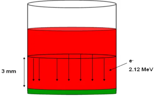
For the first check, 103electrons with energy of 2.12 MeV (maximum energy of beta
particle in188Re decay) are emitted in negative z-direction from a circular section (see
Fig. 1.11) at half of the cylindric well. The energy deposition is given by: ∆E = (−dE
dz)avg · ∆z (1.2)
where ∆z is the depth along z direction, and (−dE
dx)avg is the average Stopping Power,
function of energy and type of the particle considered and function of the material used. In this check, we have water (3 mm) and tissue (6 µm). The ratio (Rdep), by Eq.
1.2, between the energy deposited in the tissue and that deposited in water is given by: Rdep = ∆ztissue ∆zwater (1.3) By using the values of the depths simulated we have: Rtheor
dep = 2.0 · 10−3. The value
obtained by MC is an energy deposition (1.3 ± 0.1) MeV in tissue and (606.1 ± 0.6) MeV in water; therefore is RM C
dep = (2.2 ± 0.2) · 10−3, in a good agreement with the
theoretical value.
Figure 1.11: First check of simulation setup.
For the second check, we use methods for the decay of 188Re, with its specific
life-time and spectra of decay products, included in GEANT4 (see Section 1.3). Figure 1.12 shows a decay visualization obtained by GEANT4. The average value and the maximum value obtained are in good agreement with literature data [12]. 188Re
simulated material. In Fig. 1.12, 188Re decays β− into 188Os∗
2,3 that decays promptly
into the first excited state 188Os∗
2,5 and a 931 keV photon. 188Os∗2,5 decays into 188Os
and a 155 keV photon.
Figure 1.12: Example of a decay simulated with GEANT4.
Figure 1.13 shows the 188Re β- spectrum from the GEANT4 simulation. Over
the typical β− spectrum it is possible to see the internal conversion picks. In fact,
the gamma decay rays, typically 155 keV, can be absorbed by electron shells. These electrons are emitted with energy gives by:
Ee− = Eγ− Eb (1.4)
where Eb is the binding energy of the atomic shell (K,L,M). Figure 1.14 shows with
more precision the 152 keV (shell M), the 142 and 144 keV (different levels of L shell) and finally the 81 keV (K shell) peaks.
hst1beta Entries 1125024 Mean 0.697 RMS 0.4717 E (MeV) 0 0.2 0.4 0.6 0.8 1 1.2 1.4 1.6 1.8 2 2.2 Counts 0 20 40 60 80 100 3 10 × hst1beta Entries 1125024 Mean 0.697 RMS 0.4717 Re188 beta spectrum
Figure 1.13: 188Re β− spectrum. E (MeV) 0 0.02 0.04 0.06 0.08 0.1 0.12 0.14 0.16 Counts 0 10000 20000 30000 40000 50000
Re188 beta (I.C)
Figure 1.14:
For the last check, to understand the effect of the medium surrounding the cells, we have first simulated two layers of cells at equal distance from the source, one close to a plexiglas layer and the other without it (Fig. 1.15a). The inner volume of the cylindric well is filled with a solution containing188Re (red color in the Fig. 1.15). The
result of simulation is a much lower energy deposition (30% less) in the cell without the plexiglas layer. To restore the symmetry we added a plexiglas layer as show in Fig 1.15b. We have obtained respectively (297.8 ± 0.3) MeV and (298.3 ± 0.3) MeV for the top and bottom tissue layers.
Figure 1.15: Third check of simulation setup.
We can conclude that all the results of the cross-checks show a good agreement with the expected values.
1.4.3
Results
To calculate the total dose absorbed by the cells, a computation of the average dose per 188Re decay has been carried out using 106 simulated events. At this point, the
dose corresponding to a given initial activity inside the active wells can be inferred by a simple rescaling.
Considering that the lifetime (τ ) of 188Re is 24.5 hours, and indicating with A 0 the
initial activity, by using the formula:
A(t) = A0· e−
t
τ = dN
dt (1.5)
we obtain that the total number of decays (Ntot) inside the solution containing 188Re
in 48 h (72 h) is: Ntot = A0· Z 48h 0 ·e −t τ = A0 · (1 − e−48hτ ) (1.6)
An initial activity in the solution of 50µCi/cc corresponds about to 1.4×10¹¹Bq/cc
(1.6 × 10¹¹Bq/cc) in 48h (72h). Being the volume of the radioactive solution contained
within each well 0.23 cc, we obtain 3.2 × 10¹⁰ Bq (3.6 × 10¹⁰ Bq).
The GEANT4 simulation estimates an average energy deposition in the biological sample of about 280 eV per event. Therefore, the dose absorbed in 48 h (72 h) by each of the cell cultures deposited in the wells when the activity of the radioactive solution is 50 µCi/cc can be estimated as being approximately 6.3 Gy (6.9 Gy). Doses two and three times that large correspond, respectively, to the wells in the experimental setup filled with an initial activity of 100µCi/cc and 150µCi/cc.
It has been verified with the same GEANT4 simulation that, having the wells filled with the absorbing medium interleaved with the activated ones, it is possible to reduce the dose received from the nearby active cells to a negligible level. This is shown in Fig. 1.16 where the average dose deposited per event in the nearby wells, when only one of them is activated, is calculated using 108 simulated events.
Figure 1.16: Average dose, in eV, deposited in the nearby cells when only one of them in the setup is activated.
Values below 10 meV, in nearby wells, are obtained with this setup, to be compared to the average energy deposition of 280 eV for a 188Re decay inside the same well.
1.5
Experimental biodistribution
To study the effect of metabolic radiotherapy in small animals (mice), a small high-sensitivity γ-camera [32] has been built, following the experience of yttrium aluminum perovskite (YAP) camera [33][34] which is routinely used to image mice with 99mTc
HA at the Laboratori Nazionali di Legnaro, Italy (e.g. [6]).
Figure 1.17 shows the experimental apparatus, as it is used in the laboratory. The γ-camera is based on a matrix of 66 × 66 Cerium doped YAP (YAP:Ce or YAlO3:Ce)
crystals [35], each measuring 0.6 × 0.6 × 10 mm3, with 5 µmm thick optical insulation
between them. A Field Of View (FOV) of 40 × 40 mm2 is thus achievable. The
with a 3 in. diameter photocathode. The anode consists of 16 plus 16 wires, crossing at 90◦ and connected by two resistive chains, defining the x and y directions. A 40 mm
thick lead parallel hexagonal holes collimator [37], with hole diameter 1.5 and 0.18 mm septa, is placed in front of the YAP matrix. The detector is triggered using the last dynode and the ends of the x and y resistive chains. Its signals are amplified, stretched and read out by a NI 6023E card [38] connected to a Personal Computer (PC). All collected data are saved event by event in files stored on a hard disk for the offline analysis.
Figure 1.17: The experimental apparatus which is taking data at INFN in Legnaro (Padua - Italy). On the right one can see the mechanical structure and source positioning system, which contains the scintillator, the PM and the collimator inside the cylinder. The rack containing the readout electronics is visible on the left.
1.5.1
Energy resolution of the YAP camera
The energy response of the camera is calibrated as a function of the source position. For the calibration, a flat field of a solution containing 99mTc is taken, and the measured
energies of the 140 keV photon are all equalized to the same value, everywhere in the FOV of the camera. The energy resolution (ER) of the setup, is thus determined by using a 6.8 mm diameter and 10 mm height plastic well filled with a solution with ∼0.3 GBq of188Re activity. This well is put under the YAP camera setup and data are
acquired during 3 h. The total energy spectrum obtained from all the points originating from within the position of the well Region Of Interest (ROI) is shown in Fig. 1.18.
Figure 1.18: The total energy of a cylindrical188Re source measured in the YAP-camera.
In the horizontal axis, the photon energy is expressed in arbitrary units, while in the vertical axis the corresponding counts are listed.
For the 155 keV 188Re line, the energy resolution obtained in that way is 40% Full
Width Half Maximum (FWHM).
1.5.2
Spatial resolution of the YAP camera
The digital-to-length conversion factor is determined using a set of three parallel cap-illaries, 0.7 mm wide and spaced 1.0 and 1.5 cm apart, filled with a solution of 99mTc.
The image obtained from them is visible in Fig. 1.19. The Spatial Resolution (SR) obtainable in the present YAP camera setup with 188Re, at 10 mm distance from the
collimator is then determined by acquiring an image (as in Fig. 1.20) by using the same well described in Section 1.5.1. The SR is measured separately in the horizontal and in the vertical directions by deconvoluting a Gaussian shape from the known geometrical shape of the well in thin horizontal and vertical slices [39]. The results give a FWHM of (2.76 ± 0.10) mm in x and (2.72 ± 0.10) mm in y.
To increase the SR without losing sensitivity, and to obtain different projections simultaneously, we are building two new cameras to be positioned at 90◦ around a
small animal. To obtain the biodistribution and tomographic information, they use as scintillators two planar crystals of LaBr3:Ce, 50 × 50 mm2 wide and 4 mm thick, read
out by one H8500 Hamamatsu Flat panel PM each, with a glass window 3.0 mm thick protecting the crystal. The front-end electronics for the 64 channels of the H8500 has been designed using MPX-08 [40] chips. The system will be mounted on a rotating support, in order to produce tomographic images.
The different emission properties of 188Re, compared to 99mTc, which emits just
one single γ-ray at a fixed energy of 140 keV, imply a different design of the imaging camera. The higher image background is due to both β-rays and higher energies γ-rays interactions.
detec-tors based on scintillation arrays of pixellated crystals [41].
Figure 1.19: Image obtained with three capillaries filled with a solution containing99mTc.
(0.7 mm inner diameter, at a distance of 10 and 15 mm from each other)
Figure 1.20: Image obtained with a plastic well of cylindrical shape, with a base diameter of 6.8 mm and a height of 10 mm, filled with a solution of 188Re. The activity of the liquid
The better ER is expected to ease the separation of the 155 keV line of 188Re
with respect to the background photons produced in a large fraction of that isotope decay. Ongoing developments of the studies aimed at optimizing the imaging of 188Re
in vivo are presented in next Chapter, including the characterization of the PM and the scintillator.
1.5.3
First measurements with
188Re
The labelling reaction of HA using 188Re is carried out with good yields (65 - 70%)
[42]. The radiolabelled compound was purified with a size exclusion chromatographic method before being used for biodistribution studies. Stability studies in rat serum confirmed the maintaining of the188Re linked to the polymer and there was no evidence
of radio-decomposition after a few hours [42].
To test the full chain, from the radiolabelling to the imaging “in vivo”, a C57 black mouse (healthy, female) has been injected with188Re-HA [4]. After general anesthesia,
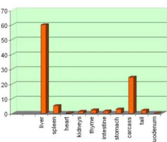
the solution with an activity of about 250 µCi is injected in the caudal vein. The mouse is positioned along the diagonal of the FOV, with the locus of injection outside it, and is monitored for about three hours. The image collected in the first five minutes shows a large spot close to the locus of injection in the tail (Fig. 1.21).
After 5 minutes, the activity concentrates roughly in the centre of the body, in a volume which contains the liver (Fig. 1.22). The activity is slowly decreasing during the 3 h of the measurement. After 3 h the mouse is sacrificed, and the organs are extracted and measured with a microcurimeter (Fig. 1.23). The liver contains 60% of the residual activity and close by organs another 20%, in agreement with the scintigrafic image (Fig. 1.22), where individual organs are not resolved.
Figure 1.21: The image of the C57 mouse integrated for the first 5 minutes after the injection of188Re- HA in the caudal vein.
Figure 1.22: The image of the C57 mouse integrated between 5 and 185 minutes after the injection of 188Re-HA in the caudal vein. The volume of large activity corresponds to the
Figure 1.23: Activity of various organs “post mortem”.
Even with limited resolution the test shows that it is possible to monitor the biodis-tribution of188Re in mice, with a potential saving in the number of animals needed for
Chapter 2
Lanthanum Bromide Crystals
2.1
Introduction
Over the last few years scintillation crystal machining has greatly improved. At the same time new scintillating crystals suitable for Medical Imaging have appeared on the market. It is possible to built Sodium Iodide doped with Thallium (NaI:Tl) arrays with about 1.0 - 1.1 mm pixel size and good light output, or Cesium Iodide doped with Thallium (CsI:Tl) scintillation arrays with sub-millimeter pixel size. The main limitation offered by scintillation arrays is the SR as limited by pixel size and the ER response limited by dead zones between crystals pixels. In continuous and pixellated crystals, the scintillation event position is usually calculated by the Anger algorithm [43], which determines the location of each scintillation event, as it occurs, using the weighted average of signals coming from the photodetectors that operate the sampling of the scintillation light distribution. The possible limitation to the use of continuous crystal is the bad linearity (L) response, and as a consequence the poor SR, which arises in small FOV gamma cameras assembled with planar crystals [44].
A LaBr3:Ce scintillation crystal cannot be machined in small pixel size, since it
is fragile. It has a light yield (LY) almost twice higher than NaI:Tl (see Table 2.2) and it has very similar absorption radiation properties and refraction index as NaI:Tl (see Table 2.1). To understand better the potentials of this scintillation crystal in gamma ray imaging, a more complete study of different continuous LaBr3:Ce crystals,
performed by GEANT4 simulations, is described in the following. In particular the work is focused on the scintillation light distribution and how they affect L.
2.2
Lanthanum Bromide features
The scintillation properties of LaBr3 doped with 0.5% Ce3+ have been presented for
the first time in 2001 by Delft and Bern Universities. The peculiar features of LaBr3:Ce,
vs other crystals, are shown in Tab.2.1 and 2.2 (see also [45]).
In Fig. 2.1 the absorption curves are shown as a function of LaBr3:Ce crystal
thickness and of γ-photon energies. Intrinsic efficiency (@ 140 keV) is 80% and 70% respectively for 5 mm and for 4 mm thick crystals. The 137Cs spectrum, published by
Saint Gobain [46], shows ER of 3% at 662 keV (Fig. 2.2).
Table 2.1: LaBr3:Ce and NaI:Tl properties: attenuation @ 140 KeV
Decay Time (ns) Att. Len. (mm) λ Max (nm)
Labr3:Ce 16 (97%) 3.6 380
NaI:Tl 230 4.9 410
BGO 300 0.8 480
CsI:Tl 1000 2.4 550
Table 2.2: LaBr3:Ce and NaI:Tl properties, refractive @ λ Max
Density (g/cm3) LY (ph/MeV) Refractive Index
LaBr3:Ce 5.3 63000 1.90
NaI:Tl 3.7 38000 1.85
BGO 7.1 9000 2.15
CsI:Tl 4.5 52000 1.79
LSO 7.4 28500 1.82
Figure 2.1: Absorption curves (%) in a LaBr3:Ce as a function of gamma-ray energy and
Figure 2.2: 60Co spectrum (Saint Gobain) measured with a LaBr3:Ce crystal.
2.3
Experimental setup
Preliminary tests are performed on a crystal (48 × 48 × 4 mm3). The crystal (Fig. 2.3)
is covered on the front and lateral side with an aluminium case (0.5 mm thick), while on the back side it is coupled to a single Flat Panel Position Sensitive PM through an optical glass window 3 mm thick.
Figure 2.3: Side view of the LaBr3:Ce planar crystal assembly.
The front surface is covered with white diffusive reflector (Teflon 0.3 mm thick) in order to reflect the light output emitted opposite to the PM and increase the light
output. A black light absorber is placed on the lateral surfaces of the crystal and of the glass proctecting the crystal (CG) lateral surfaces to avoid light reflections which will cause Point Spread Function (PSF) distortions. The Hamamatsu H8500 Flat Panel PM [36] has an external size of 52 × 52 × 27.4 mm3. A bialkali photocathode and 12
stages metal channel dynode are used as electron multiplier. A 8×8 matrix anode (64 channels), with pixel size of 5.8 × 5.8 mm2, is used for a position sensitive function in
which each individual pixel has a 6.08 mm pitch. The overall active area is 49.0 mm squared. The PM is characterized by a glass window thickness (PMG) of 1.5 mm, an anode dark current of 1 nA and by an anode gain variation range of about 45:100. The PM gain is about 1.5 · 106 at -1100V and the quantum efficiency (QE) of the PM is
27% at the peak of the emission spectrum of LaBr3:Ce, according to the manifacturer’s
design specifications (see Fig. 2.4).
2.4
Photodetection principle
The 8 × 8 anodic array of the H8500 (MA-PMT) is shown schematically in Fig. 2.5, where nk
j represents the charge signal readout on the k-th row and j-th column of
the anodic array. SR depends on the the statistical uncertainty of the scintillation position measurement. Such a position is determined by using the MA-PMT and a centroid algorithm ( “linear”) elaborated by Anger in 1958 that it is, still now, the basic principle of imaging reconstruction in modern scintillation gamma cameras [43]. The centroid algorithm calculates the position (X,Y ) of the scintillation event by the average values of the measured charge distributions, which represents a point in the imaging plane. Many γ-ray interactions then give rise to the image of the emitting source.
Figure 2.5: Schematic drawing of the anodic structure of the H8500.
The “linear” algorithm applied on a charge distribution can be written as follows: XC = P jnjxj P jnj (2.1)
where nj =
P
knkj is the “projection” of the charge collected along the j-th column, xj
is the anode coordinate and Xc is the centroid coordinate along the x-direction. The
same applies along the y direction: YC = P knkyk P knk (2.2) here nk = P
jnkj is the “projection” of the charge collected along the k-th row, yk is
the anode coordinate and Yc is the centroid coordinate along the y-direction.
SR relates to the ability of the imaging system to distinguish between two closely spaced objects on an image; in particular SR is the minimum distance between two point sources that are reproduced as distinct by the detection system and it is related to the statistic uncertainty of the scintillation event position σ2
XC (σ
2
YC) of the Xc (Yc)
coordinate of the scintillation event. By applying the statistical definition of standard deviation σ2 XC (σ 2 YC) we can write: σXC = σcharge √ nphe (2.3) Where σcharge represents the standard deviation of the charge distribution as projected
along x direction ( y direction for σYC), and nphethe average number of photoelectrons.
So the SR of the detector measured as FWHM, is: SR = F W HMP SFimage =
F W HMcd
√n
phe
(2.4) where F W HMcd = 2.35 · σcharge is the full width at half maximum of the projected
charge distribution.
A “quadratic” algorithm [47] has been used applying a squaring procedure to the charge distribution collected from MA-PMT. The “linear” algorithm is modified by the following: XC = P jn0jxj P jn0j (2.5)
with n0 j = X k (nk j)2 (2.6)
Experimental values are influenced by a light background into the crystal, which affect σcharge and consequently also SR. For all reconstruction algorithms, it is possible to set
a threshold (t) useful to remove the light background. Eq. 2.6 becomes: n00 j = X k (nk j − t)2 (2.7)
and the “quadratic” algorithm:
XC = P jn00jxj P jn00j (2.8)
In Fig. 2.6, we show the PSF of light (PSFlight) coming from an ideal (without
fluc-tuations) scintillation event and the image (PSFimage) obtained from many scintillation
events.
Figure 2.6: The PSF of an ideal scintillation event (left) and a PSF image as due to the many scintillation (right).
In Fig. 2.7 is shown the reconstruction technique from an ideal scintillation event made of three principal steps needed to obtain the X and Y position of each scintillation
event. In in Fig. 2.7a. the light scintillation spread. In Fig. 2.7b the MA-PMT operates a sampling of the PSFlight obtaining the charge distribution shown. In Fig. 2.7c the
charge projection along one direction.
Figure 2.7: Reconstruction technique from an ideal scintillation event a) Light scintillation spread. b) Charge distribution as sampled by the anode array. c) Charge projection along one direction, ready to apply the centroid algorithm.
2.4.1
Linearity and Spatial Resolution
L relates to the ability of an imaging device to reproduce linearly the displacements of a radioactive source across the face of the detector. It can be visualized by plotting real (or mechanical) position versus measured position (Fig. 2.8).
L is defined as:
L = ∆Xmeasured ∆Xmechanical
(2.9) which represents the angular coefficient of L curve at each measured point. L is then useful to describe the deviation from a perfectly linear behaviour (L=1) and represents
a calibration to convert distances reproduced in the image to the “real” distances of the object [48].
Figure 2.8: Light edge effect.
In the Anger Camera, L is affected by the edge effect, since when gamma-rays interacts at a point in the crystal near the boundary, the charge distribution shape is altered and the mean position estimated by the centroid algorithm is no more equal to the maximum of the light distribution (Fig. 2.8). A good L means then that the centroid algorithm reproduces correctly the real (mechanical) position. A bad L causes image compression and worsen the SR. In fact, assuming a poissonian distribution for nk j, we define SR by: SR = 1 L· F W HMcd √n phe (2.10) In Section 2.6 we will calculate FWHM of the charge spread distribution, L and SR by applying “linear” and “quadratic” algorithms on a photoelectrons distribution,
using simulated and experimental data.
2.4.2
Energy Resolution
The ER is defined as the full width (∆E) of the peak in the pulse height spectrum at half the maximum intensity, divided by the central energy value:
ER = ∆E
E (2.11)
ER is an important parameter for imaging devices since image contrast mainly relates to the ability of the detector of discriminating between photopeak events and Compton-diffused photons. When spectrometry measurements are performed with scintillators optically coupled to photomultiplier tubes, ER is proportional to the standard deviation of the charge that reaches the anode in each scintillation event. Charge production consists of five sequential processes each dependent on the previous one that can be described as follows:
• Production of scintillation photons in the crystal due to gamma-ray interaction; • Collection of scintillation photons at the PM photocathode;
• Production of photoelectrons in the photocathode due to incident scintillation photons;
• Collection of photoelectrons at the first dynode in the PM; • Multiplication of electrons by the dynodic chain.
ER can be parameterized [49][50] as:
where ERint is an additional intrinsic resolution which has been interpolated from
experimental data in [50] for LaBr3:Ce and yields (4.5 ± 0.5)% for 140 keV photons.
ERsta represents the Poissonian component of ER given by the square root of the
number of collected photoelectrons. The variance of the electron multiplier gain [50] is not taken into account in the calculation of the total energy resolution.
The intrinsic component of ER was first observed in 1956 (Kelly et al.). Since then onwards a lot of studies [51][52], recently [53], have investigated the origin of this non poissonian contribution which still represents the main limitation to the overall ER. The exact mechanism has not been fully explained yet, nevertheless some conclusions are to date widely accepted :
• differences in light production at different crystal locations, probably due to crys-tal lattice defects;
• crystal growth methods used by the manufacturer for production of “large crystal size”.
In addition to the intrinsic energy resolution, the scintillation light yield is affected by a non proportionality of the emitted light with energy of gamma ray released to the crystal. This effect is main related to the type of interaction.
2.5
Simulation setup
For the modeling of the electromagnetic interactions, the “Penelope” [54] model avail-able with GEANT4 (4.9.0 version) is used. Atomic relaxations following photoelectric effect, Compton scattering, ionization interactions, Rayleigh scattering, fluorescence photons and Auger electrons are simulated. GEANT4 allows also the transport and boundary effects for the optical photons (see appendix A) generated by the
scintillat-ing crystal to be simulated. Figure 2.9 shows the simulated set up by GEANT4. The simulated scintillation camera reproduces the geometry of the experimental setup (see Section 2.3). The CG and PMG, respectively 3.0 mm and 1.5 mm, are composed of the same glass material (same optical proprieties). Initially, to emulate the black light absorber wrapping the experimental crystal and the CG, the ref lectivity (R) of the lateral surface of the simulated crystal has been set equal to zero. As explained in the following (see Section 2.6), it is found, comparing with the experimental data, that a certain amount of light is reflected in fact, and a different value of R is used for the final simulation setup.
Figure 2.9: The set up used in the simulation.
photons reaching the readout surface in a grid of 8×8 squares. The QE of the PM is em-ulated by setting the surface between PMG and PM (active area) as dielectric − metal with an ef f iciency of 0.27. In the simulation, the boundary processes of all crystal sur-faces follow the rules of the UNIFIED model, developed for the DETECT project [55]. The optical properties of the materials involved in the simulations (refractive index, absorption and scattering lengths) are gathered from literature [56]. A scintillation light yield equal to 63000 photons/MeV is assumed for LaBr3:Ce. The scintillation
photons are generated as a pure Poisson process (resolutionscale = 1, see Appendix A). In Fig. 2.10 we show the scintillation photons produced by an interaction of an 140 keV energy photon into a LaBr3:Ce crystal1.
Figure 2.10: The set up used in the simulation including a sketch of optical photons.
In the UNIFIED model some combinations of surface properties, such as Polished
1For a correct and clear visualization of the optical photons, a scintillation light yield equal to 60
or Ground, enumerate the different situations which can be simulated. In all cases, the surfaces are made up of micro facets with normal vectors that follow a given distribution (see Fig. 2.11). The angle between a micro-facet normal and the average surface normal, α, is assumed to follow a gaussian distribution of standard deviation σα and n1, n2are respectively the indexes of refraction of the incident and transmission
medium.
Figure 2.11: Micro-facets and average surface.
The Polished model is meant to account for a perfectly polished surface. Photons incident on the surface are assumed to have random polarization, and are first tested for the possibility of Fresnel reflection if a change in refractive index occurs at the surface. If reflection does not occur, the optical photon is transmitted with the complementary probability given by:
T = 1 − R (2.13)
If reflection occurs, the angle of reflection is set equal to the angle of incidence (Fig. 2.12 on the left).
The Ground option is available to simulate a rough or ground optical surface. It is treated in the same way as the polished surface described above, except that the reflection (refraction) follows a Lambertian distribution. (Fig. 2.12 on the right).
Figure 2.12: Modelization of the reflection on the surface of the scintillating crystal: Polished (left) and Ground (right).
In the simulation to emulate a completely white diffusive experimental surface, the LaBr3:Ce front surface has these (optical) parameters:
• dielectric − metal; • ground; • R = 0.95; • σα = 0.0; • Cdl = 1; • Csl = Css = Cbs = 0;
where Cdl is the diffuse lobe constant for the probability of internal Lambertian and
about the normal of a micro facet, the Css is the specular spike constant illustrates
the probability of reflection about the average surface normal and finally Cbs is the
back-scatter spike constant for the case of several reflections within a deep groove with the ultimate result of exact back-scattering.
We apply the Snell’s Law for the surface between crystal and CG. For the lateral surfaces of the PMG we set R = 0.0 2.
For more details about the simulation of optical photons, see Appendix A.
2.6
Results
First of all, using GEANT4 we have simulated a pencil beam of 140 keV photons3
impinging the crystal (at the centre), and we have calculated the average depth of interaction within the LaBr3:Ce crystal (located at about 2.33 mm from the crystal
back surface as shown in Fig. 2.13).
The gamma generates some optical photons as shown in Fig. 2.10. Some of them travel directly through the CG and PMG windows towards the PM. Some others are reflected by the lateral surfaces or by the front side of the crystal. In this first test, all the surfaces of the setup are supposed complectly black (total absorption of the optical photons, using R = 0). The fraction of optical photons (starting from the interaction point) moving towards the CG resulted to be (44.9 ± 0.4)% in the simulation. In the theoretical expectation, based on purely geometric arguments (see Fig. 2.13), considering the angle θcry = arctg(24.02.33), it is possible to obtain the fraction of optical
2When R = 0.0, it is not necessary to specify all other optical proprieties.
3The energy of the γ-ray produced in the99mTc decay. This energy value is the same used for the
Figure 2.13: Simulated average interaction point in the LaBr3:Ce crystal.
(fopt) using the formula:
fopt(%) = 100.0 ·
∆Ω
4π (2.14)
where ∆Ω is given by:
∆Ω = 2.0 ·
Z θcry
0
Z 2π
0 sin(θ)dθdϕ (2.15)
Considering the limit angle given by:
θlim = arcsin(
nglass
ncry
) (2.16)
the expected fraction of optical photons moving towards the PM is 19.0%, to be compared with an MC value of (18.8 ± 0.2)%.
As we have seen in Section 2.4, by MC it is possible to show the effects on the charge distribution using “linear” or “quadratic” algorithms with or without threshold level. Figure. 2.14 and Fig. 2.15 show respectively the charge distribution spread for a single gamma central and lateral interaction. In particulary, Fig. 2.14b and 2.15b show the effect of a threshold level (5% of the maximum) on the charge distribution
and in Fig. 2.14c and Fig. 2.15c the squared charge distribution (with threshold) are shown.
Figure 2.14: Simulated charge distributions (central interaction).
Figure 2.15: Simulated charge distributions (lateral interaction).
The better reconstruction of interaction point by “quadratic” algorithm (with a threshold) is clearly evident mainly for a lateral interaction (in the Fig. 2.15c with
respect to Fig. 2.15a).
In the second test, we have calculated (Figure 2.16) the number of detected optical photons in correspondence of different R values of the crystal and CG lateral surfaces, using dielectric − metal and the polished model4. Photons interact at the centre and
at the border of the crystal. In our experimental setup, the light collected when the source is near the edges is about 80 − 85% of that collected when the source is at the center. This experimental result can be possible only if the considered lateral walls are not perfectly black. In fact, in case of total absorption, one should expect instead that the light collected when the source is located near the edges of the crystal is roughly half of that collected when the source is at the center of the crystal (as visible in Fig. 2.16).
Figure 2.16: Number of detected photons with the gamma impinging at the centre and at the border of the crystal, as a function of the reflectivity of the crystal and CG lateral surfaces.
Considering the optical parameters just set in the simulation setup, described in Section 2.5, we found a (preliminary) agreement between experimental and simulated
4In this case: C
data using (for the crystal and CG surfaces next to aluminum wrapping):
• dielectric − metal • Polished model; • σα = 0.05
• R = 0.6;
As a consequence of the preliminary results, we have to assume that the considered lateral surfaces are indeed not perfectly black, and they could reflect back some amount of light. To verify this statement, we have decided to use a comparison with the experimental data by using the sigma (σpcd) [47] of the projection (on one of two read
out coordinates) of the collected charge distribution, event by event. We have simulated the LaBr3:Ce crystal (and CG) with lateral walls reflection coefficients varying from
0.5 to 0.8. The results obtained are shown in Fig. 2.17 where the sigma values of the simulations, done with R = 0.5, 0.6, 0.7 and 0.8, are compared with the experimental data.
These sigma values are evaluated from the charge distributions obtained using a pencil beam impinging both at the center and at the border of the crystal. For every step of R, 4·104photons of 140 keV are used6. We observe again that the experimental
and simulated data agree well, with one another, for a value of R = 0.6 (see also Fig. 2.18).
We can conclude that the crystal and the CG used for our experimental measure-ments has not the ideal optical properties we expected, but we can suppose instead that the lateral surfaces reflect scintillation light back into the crystal.
5We have supposed that polished surface are perfect. 6Optical photons simulations need a lot of CPU time.
Figure 2.17: σpcd comparison for simulated and experimental data at the center and at the
boundary of the crystal. The simulation is performed with different reflectivity values.
Figure 2.18: Monte Carlo (Polished model, R = 0.6) vs experimental data: charge distribuition spread @ 140 keV.
To study other possible crystal configurations, in view of looking for the most performant gamma camera based on LaBr3:Ce crystals, three different crystal assembly
are simulated: “Ground”, “Polished” and “Air Gap”. “Ground” and “Polished” refer to the status of the lateral surfaces of the crystal and of the CG, as already discussed, while “Air Gap” is the “Ground” model with a thin air interface (0.1 mm) between the CG and the PMG. For every model, the front surface is the same just described in Section 2.5. For the “Ground” model, we have used for crystal and CG lateral surfaces:
• dielectric − metal and ground model; • σα = 0.0;
• Cdl = 1 and Csl = Css = Cbs = 0.;
Figures 2.19 2.20 and 2.21 show the energy spectra obtained by a central interac-tion in the crystal, respectively for “Polished”, “Ground” and “Air Gap” model, with superimposed a gaussian fit.
Figure 2.19: “Polished” model: energy spectrum with superimposed a gaussian fit (continuous line).
Figure 2.20: “Ground” model: energy spectrum with superimposed a gaussian fit (continuous line).
Figure 2.21: “Air Gap” model: energy spectrum with superimposed a gaussian fit (continuous line).
The crystal is scanned using a pencil beam impinging different positions with 2 mm step. For every step, 2 · 104 photons of 140 keV are used. Figures7 2.22, 2.23 and
2.24 show the profiles of the scanning performed by “linear” (left) and the “quadratic”
(right) algorithms, respectively for “Polished”, “Ground” and “Air Gap” models. The better “visibility” of the profiles, obtained by weighting the central anode position with the quadratic algorithm (right) is evident.
Figure 2.22: “Polished” model: the profiles of the scansion performed with a pencil beam impinging different positions with 2 mm step, using “linear” (left) and the “quadratic” (right) algorithms.
Figure 2.23: “Ground” model: the profiles of the scansion performed with a pencil beam impinging different positions with 2 mm step, using “linear” (left) and the “quadratic” (right) algorithms.
Figure 2.24: “Air Gap” model: the profiles of the scansion performed with a pencil beam impinging different positions with 2 mm step, using “linear” (left) and the “quadratic” (right) algorithms.
Experimentally, the crystal is scanned with 0.4 mm collimated 99mTc spot source
with 2 mm step. Fig. 2.25 compares the determination of the position as obtained, in the three optical models, with the “linear” and the “quadratic” algorithms. The better L value obtained by weighting the central anode position with the “quadratic” algorithm is clear, even if the non-linearity at the edges is still present. The SR analysis, comparing MC and experimental data, is shown in Fig. 2.26 that shows three different interaction points (step 2 mm) at the centre of the crystal.
Finally, the ER values, the average number of photoelectrons gained by anode, SR and L are respectively summarized in Table 2.3, Table 2.4 and Table 2.5. The statistical values (ERstat) of ER, obtained by MC simulation, are affected by a negligible error
with respect to the intrinsic one. For this reason, these errors are omitted and the error on ERM C is calculated only from the intrisic ER, (4.5 ± 0.5)%. The SR and ER
values obtained correspond to the source position in the center area of the crystal. In the tables, SRlin, SRqua Llin and Lqua represent the SR and the L obtained by applying
linear/quadratic (with threshold) algorithm.
Figure 2.25: L values for the three setup described in the text. These values are obtained using either the “quadratic” or the “linear” algorithm.
Table 2.3: Photoelectrons and Energy Resolution
Setup < Nphe > ERsta % ER %
Exp. - - 9.0 ± 0.3
Polished 1047 ± 1 7.2 8.6 ± 0.3 Ground 1603 ± 1 5.9 7.4 ± 0.3 Air Gap 1137 ± 1 7.0 8.3 ± 0.3
Table 2.4: Spatial Resolution (central interaction)
Setup SRlin (mm) SRqua (mm)
Exp. 1.6 ± 0.1 1.1 ± 0.1 Polished 1.2 ± 0.1 0.77 ± 0.04
Ground 1.0 ± 0.1 0.75 ± 0.04 Air Gap 1.5 ± 0.1 0.8 ± 0.1
Table 2.5: Position Linearity
Setup Llin (mm/mm) Lqua (mm/mm)
Exp. 0.65 ± 0.05 1.00 ± 0.05 Polished 0.67 ± 0.05 1.02 ± 0.05 Ground 0.70 ± 0.05 1.01 ± 0.05 Air Gap 0.55 ± 0.05 0.99 ± 0.05
The L coefficients (Table 2.5) are calculated not considering the last three values near the crystal border (Fig. 2.25). As we can see in the tables, the simulation results for “Polished” model, which corresponds to the crystal surface treatment made by St.