Experimental Characterization of Full Field Creep Deformation in Adhesively Bonded Joints

(1)

UNIVERSITÀ DI PISA

DIPARTIMENTO DI INGEGNERIA CIVILE E

INDUSTRIALE

Tesi di Laurea Magistrale in Ingegneria Aerospaziale

EXPERIMENTAL CHARACTERIZATION OF FULL

FIELD CREEP DEFORMATION IN ADHESIVELY

BONDED JOINTS

Relatori:

Prof. Ing. Giorgio Cavallini

Ing. Roberta Lazzeri

Prof. Satchi Venkataraman

Candidato:

Jacopo Casini

ANNO ACCADEMICO 2012/2013

(2)

ii

ABSTRACT

Structural adhesives employed in bonded joints are polymers, whose deformation and stress exhibit time and temperature rate dependence. Creep is the tendency of a solid material to slowly move or deform permanently under the influence of stress. Understanding creep behavior of adhesive materials is critical to establish the life and the durability of adhesively bonded structures.

This research aims at the experimental characterization of adhesively bonded joints creep deformation through the application of a full field measurement system.

The project can be divided in 3 parts:

1) design and manufacturing of test facilities and specimens,

2) preliminary tests to assess specimen, fixture and measurement method tests repeatability and consistency,

3) carrying out of creep tests on adhesive materials: creep properties are obtained by subjecting adhesively bonded aluminum butterfly shaped specimens to biaxial loads using an Arcan fixture and a heat chamber.

The objective is to characterize adhesive creep response in a joint configuration which is tested under a controlled stress state and at the same time is close to real joints behavior. Such data could be used for validating the analytical predictions on single lap bonded joint behavior, showing at the same time the possibility for a computational model to be comparable to the tests results. On the other hand the use of full field measurements will guarantee a deep analysis of the whole joint adhesive section, which could not have been possible with traditional mechanical measurement systems.

(3)

iii

List of Tables

Table 4-1: Aramis properties, ... 24

Table 4-2: Noise data at room temperature ... 30

Table 4-3: Glass door noise check results ... 31

Table 4-4: Spatial resolution parameters... 34

Table 4-5: Noise check and filter summary. ... 36

Table 5-1: List of devices and materials for chromic acid etching ... 45

Table 5-2: Nominal dimensions of bonded butterflies, mm ... 48

Table 5-3: Static test & bond area dimensions resume. ... 49

Table 5-4: Hysol® EA 9394 adhesive and butterfly specimen properties ... 50

Table 6-1: Bonded butterflies creep test summary. ... 60

Table 6-2: Creep parameters fit summary ... 62

List of Figures

Figure 1-1: All composite wingbox structure ... 1

Figure 1-2: Adhesive section analytical stress distribution... 2

Figure 1-3: The Arcan fixture designed and manufactured for this project. ... 3

Figure 1-4: Non-uniform stress state on ASTM D3165 ... 4

Figure 1-5: Bonded butterfly under 24 MPa in a pure shear load static test. ... 4

Figure 2-1: Creep strain vs time typical curve ... 6

Figure 2-2: ASTM E1640 dynamic mechanical Tg test. ... 7

Figure 2-3: a) Maxwell and b) Kelvin-Voigt models ... 8

Figure 2-4: Four element Burger’s model. ... 9

Figure 3-1: ASTM D1002 dimensions. ... 12

Figure 3-2: ASTM D3165 dimensions, mm. ... 12

Figure 3-3: Volkersen shear lag model for SLJ. ... 13

(6)

vi

Figure 3-5: ASTM specimen deformation under tension loads. ... 16

Figure 3-6: D3165 Shear (top) and normal (bottom) DIC strain state at 1350 N ... 17

Figure 3-7: Shear and normal strain measurements along bondline central section. .. 17

Figure 3-8: Failure modes for adhesive join design. ... 18

Figure 3-9: The original Arcan fixture showing the uniformity of shear stress ... 19

Figure 3-10: The modified Arcan fixture design. ... 19

Figure 3-11: Popelar & Leichti modified Arcan fixture and specimen with LVDT configuration. ... 20

Figure 3-12: Possible mold configuration for bonded butterflies specimens. ... 21

Figure 3-13: Bulk Aluminum 6061 butterfly check for strain uniformity ... 22

Figure 4-1: ARAMIS DIC set up on Arcan fixture ... 23

Figure 4-2: Calibration measuring parameters. ... 25

Figure 4-3: Linear shape function behavior ... 27

Figure 4-4: Aramis report of a pure shear test ... 27

Figure 4-5: Examples of spray patterns ... 28

Figure 4-6: Speckled pattern on D3165 ... 29

Figure 4-7: Room temperature noise check ... 30

Figure 4-8: DIC creep glass door set-up. ... 31

Figure 4-9: Random stage points ... 31

Figure 4-10: Normal strain εx noise level for glass door... 32

Figure 4-11: Aramis noise test on glass door report ... 32

Figure 4-12: Heat chamber noise for εx and Ux ... 33

Figure 4-13: εx and Ux noise measurements through glass door after no door calibration. ... 33

Figure 4-14: Batch 2-5, stage 50, debond region ... 36

Figure 4-15: Batch 3-2, stage 172, constant shear strain ... 36

Figure 5-1: Creep test set up ... 38

Figure 5-2: Instron vibration ... 39

Figure 5-3: Arcan fixture ... 40

(7)

vii

Figure 5-5: Arcan and clevises, connected to the Instron through the rod. ... 42

Figure 5-6: Steel clevis design sheet, mm. ... 42

Figure 5-7: Steel rod design sheet, in. ... 43

Figure 5-8: Aluminum bonded butterfly nominal dimensions, mm. ... 44

Figure 5-9: Sand-papered butterflies ... 46

Figure 5-10: Bonded butterfly curing mold ... 47

Figure 5-11: Pure shear load test with strain gage on Al region ... 48

Figure 5-12: Adhesive failures for pure shear tests. ... 50

Figure 5-13: Cohesive failures ... 50

Figure 5-14: Failure shear tests summary. ... 51

Figure 5-15: Static failure stress levels along with test scatter. ... 51

Figure 5-16: Instron load vs time, specimen 5_2, pure shear. ... 52

Figure 5-17: εxy DIC data fit, with fitting 10th degree equation, pexy. ... 53

Figure 5-18: εxy vs Load, interpolated fit. ... 53

Figure 5-19: Batch 5, failure tests under shear loads on bonded butterflies. ... 54

Figure 5-22: Normal component for failure tests under mixed mode loads. ... 55

Figure 5-23: Batch 6, failure tests under normal loads. ... 56

Figure 5-24: Batch 7, failure test under normal loads. ... 56

Figure 5-25: Tension stress average response summary for batch 5,6,7. ... 57

Figure 5-26: Shear stress average response summary for batch 5,6,7. ... 57

Figure 5-27: Measurement point position. (specimen 7-6, 20 hours at 5.8 MPa)... 58

Figure 5-28: Strain phases of different points along the section ... 59

Figure 6-1: Shear creep strain versus time ... 61

Figure 6-2: Norton-Bailey power-law coefficient fit. ... 63

Figure 6-3: Mixed mode shear creep strain vs time ... 64

Figure 6-4: Mixed mode shear strain after 21 hr at 5.8 MPa (5_11). ... 64

Figure 6-5: Shear strain showing debond... 65

(8)

viii

Figure 6-7: Bondline central section after 12 hours at 3.7 MPa ... 66

Figure 6-8: Normal creep strain evolution (Figure 6-6) after debonding ... 66

Figure 6-9: Normal strain creep evolution at 30% ϭf ... 67

Figure 6-10: Normal and shear strain after 6 hours creep at 8.5 MPa ... 68

Figure 6-11: Instron crosshead displacement increase over time ... 68

Figure 6-12: DIC normal strain for 20 and 25 % ϭf. ... 69

Figure 6-13: Creep strain for debonded spec. at 25% ϭf.. ... 69

(9)

ix

List of Symbols

= Adhesive Young’s modulus, GPa = Adhesive shear modulus, GPa = Poisson’s ratio

= Tension failure stress, MPa

= Shear failure stress, MPa

= Engineering shear strain at static failure = Normal strain at static failure

= Engineering shear creep strain

₌ _{Normal creep strain, %}

̇ ₌ _{Creep strain rate}

= Glass transition temperature, °C

= Glass transition temperature in dry conditions, °C

(10)

1

1. INTRODUCTION

Structural adhesives have become increasingly important in the last 30 years both in military and civil aviation. Bonded joints are an efficient joining method for composite structures, as they are able to distribute load over a wide area without the local stress concentrations that are typical of other mechanical fastening methods. Use of bonded joints results in (1) increase in specific strength (with respect to weight, three times that of riveted joints), (2) increase in resistance to cracks and fatigue, and (3) reduction in time and cost necessary for machining and assembly procedures, [1].

Figure 1-1: All composite wingbox structure with an adhesively bonded joint between the skin and spar beam flanges (with inset showing details of the bonded joint between wing spar and skin).

Adhesives mechanical behavior, as with many polymers, is strongly time and temperature dependent. The creep behavior is of particular concern in the durability of bonded joints in aerospace structures, when the adhesive joints are cured at room temperature. Room temperature cure is chosen over high temperature cure to

(11)

2

minimize tooling requirements and/or also to mitigate against thermal stresses that may arise in these joints due to a thermal expansion mismatch between bonded parts, [2].

Figure 1-1 shows an all-composite wingbox structure from an actual aircraft in service that has adhesively bonded wing and spars cured at room temperature. The room temperature cure of epoxy adhesives results in lower stiffness (elastic and shear modulus), ultimate strength and glass transition temperature (Tgdry) properties. As explained in Chapter 2, Tgdry is a reference temperature for polymer transition from glassy to rubberlike behavior, beyond which the material loses its mechanical properties. A representative example of an adhesive used in aerospace applications is the modified two-part epoxy adhesive Hysol® EA 9394. The Tg of Hysol® EA 9394, in dry conditions, is 78 °C. For aircraft operating at tropical latitudes, the wing surface temperature can reach 66 °C (150 °F) or higher, therefore there is concern of creep response in structural adhesive used for configuration like the one in Figure 1-1.

Figure 1-2: Adhesive section analytical stress distribution (shear and peel) for aluminum adherend and an epoxy structural adhesive.

(12)

3

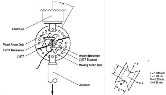
The purpose of the present work is to characterize and quantify the creep deformation of epoxy adhesive Hysol® EA 9394 to develop constitutive models that can be used to more accurately assess the integrity and durability of bonded joints. Figure 1-2 shows the stress distribution along the bondline of a single lap joint (calculated using the Goland-Reissner model, [3]), which description will be carried out in Chapter 3.1. It can be observed that the peak stresses occur at the edge of the adhesive joint and exhibit a combination of high normal and shear stress. This requires that the creep characterization of the adhesive should be performed in a biaxial (combined shear and normal) stress state. In this study, adhesive creep properties characterization was performed on adhesively bonded joints under biaxial loads using an Arcan fixture, [4] (Figure 1-3, Chapter 3.1).

Figure 1-3: The Arcan fixture designed and manufactured for this project.

Strength of adhesively bonded joints is typically characterized by using bonded lap joint specimens (e.g., ASTM 1002, ASTM D3165). These specimens, while effective for strength characterization, are not ideal for creep property characterization, due to the non-uniform shear and/or normal stresses they exhibit along the bondline and at their extremities (Figure 1-4). The butterfly shaped specimen with the adhesive joint

(13)

4

on the symmetry plane, used in an Arcan fixture, provides, along with a controlled stress state, almost uniform shear and normal stresses that are needed for the material property characterization (Figure 1-5).

Unlike dogbone or coupon specimens used for creep characterization of bulk material, adhesive bonded joints have very small material volume. Measuring global creep deformation with strain gages or LVDT’s is not ideal. Moreover, using displacement measurement gauges with Arcan fixture poses certain difficulties. In this study, the strains during creep evolution are characterized using optical methods, particularly photogrammetric methods, combined with digital image correlation (DIC), [5]: such technique is deeply explained in Chapter 4. The full field strain analysis allows the investigator to monitor the evolution of creep strain during the test in different regions of the bondline. DIC full field displacement and strain measurements provide more extensive information on the strain evolution along the adhesive joint and can be used to track the failure evolution.

Figure 1-4: Non-uniform stress state on ASTM D3165 (normal direction) composite adhesive joint specimen under 1350 N

Figure 1-5: Bonded butterfly under 24 MPa in a pure shear load static test.

Although room temperature cure results in lower strength and a more evident creep response, the latter is acknowledged for relieving edge stress peaks, which would lead to a higher durability of the joint (Chapter 3.1). Such analytical prediction, supported

(14)

5

by computational models, [6], could be confirmed by testing single lap joints specimen (Figure 1-4) under creep: DIC would register strain evolution at the edges and track down whether such relaxation is present.

The strength of adhesive joints is greatly affected by the manufacturing process, and this often leads to a large variability in measured values. Inherent to the scatter are small manufacturing defects (e.g., bondline voids), non-ideal bonding between the adhesive and adherend, due to surface preparation problems and fixture or test specimen misalignments (Chapter 5.2). In this study it is demonstrated how Digital Image Correlation based strain measurements helped identify and eliminate such problems, leading to more accurate measurements that decrease the uncertainty of material parameters identified from such measurements.

Before reaching a full creep testing capability, it was necessary a preliminary static test series (Chapter 5.3) to assess consistency in failure stress levels along with cohesive failure mode: the latter would have guaranteed the measured properties to belong to the adhesive and not to the interface with the adherend.

Creep tests were run under 40% of previously found failure stress levels for bonded butterfly configuration in pure shear, pure tension and mixed mode. Results, illustrated in Chapter 6, showed how creep response of Hysol® EA 9394 under pure shear loads is nonlinear viscoelastic, exhibiting an increased creep rate with stress. On pure tension tests side, no creep rate was tracked by DIC system: the hypothesis is that polymer chains are much smaller in thickness direction with respect to the bondline; this prevents the free volume mechanisms to activate, [7].

(15)

6

2. VISCOELASTICITY & CREEP BEHAVIOR

Creep is the tendency of a material to deform under a constant applied stress held for a period of time at chosen temperature. Such deformation is activated by energetic contribution. Metallic materials under static loads at high temperature ( Tf, fusion temperature) experience almost constant and very slow deformation rate ( ̇ _{/hr). Indeed high temperature and loads allow for dislocation} movements (even from one slip plane to another) which would have been forbidden at lower temperatures, while at reduced stresses creep is driven by diffusion phenomena, [8].

Polymeric materials creep deformation, instead, is due to weak bonds between macromolecules, [7]. Indeed the Doolitle “free volume” approach, [9], [10], relates the time scale of the material to the mobility of polymer molecules.

A typical creep curve, [11], [12], can be divided into three stages: primary, secondary, and tertiary, as shown in Figure 2-1. The secondary region is a steady-state regime at ̇ _{, where is the constant creep rate. Except at very high loads,} this phase lasts much longer than primary and tertiary (i.e., fracture) regions.

Figure 2-1: Creep strain vs time typical curve: different phases along with initial strain are plotted, [13].

(16)

7

2.1. Glass transition temperature, Tg

Adhesive properties, like with many polymers, are time and temperature dependent, [14], particularly at temperature close to their glass transition temperature (Tg). The Tg is defined as the temperature at which material storage modulus decreases sensitively (with corresponding peak in loss modulus), representing a net change in the viscoelastic response (Figure 2-2, [15]).

Figure 2-2: ASTM E1640 dynamic mechanical Tg test.

Two other Tg characterization methods are available in ASTM: one is thermomechanical (ASTM E1545) and one measures differences in heat flow (ASTM D3418). This is the reason why sometimes different laboratories measure slightly different Tg for the same adhesive.

This change from glassy to rubberlike behavior also results in decrease of mechanical properties such as Young’s modulus and shear strength. Even being close to such temperature could affect the creep response of the polymer, therefore affecting the durability of the joint, thus justifying this investigation. The two-part epoxy structural adhesive studied is Hysol EA9394, which Tgdry is 78°C. Creep tests temperature chosen was 66°C, as the highest possible temperature reached by an operating joint (wing surface at tropical latitudes).

(17)

8

2.2. Linear viscoelasticity

Experimental creep data fitting models are used in extrapolating data for engineering design. Viscoelastic response can indeed be represented with elastic and viscous components modeled as linear combinations of springs (elastic response) and dashpots (viscous response). Different arrangement of these two elements lead to different rheological models: the most important of them are listed below [16].

Maxwell: ̇ ̇ ( 1 )

which provides the following creep equation,

[ { }] ( 2 )

where is the instantaneus stress.

Kelvin-Voigt: ̇ ( 3 )

with their creep equation:

[ ( )] ( 4 )

Figure 2-3: a) Maxwell and b) Kelvin-Voigt models

The most common constitutive one is the Burger four-element model (Eq. ( 5 ) - Figure 2-4) which puts together Kelvin-Voigt and Maxwell’s models, [17]:

(18)

9

where ( ) is the time dependent strain, is the applied stress, and are the elastic modulus and viscosity of Maxwell model, and and are the elastic modulus and viscosity of Kelvin-Voigt model. The four fractions are the model parameters to be fit in the experimental data.

Figure 2-4: Four element Burger’s model.

One analytical model used to describe the behavior of viscoelastic materials employs integral constitutive relations called hereditary integrals. This approach can be used for linear materials where a superposition principle is valid. The stress-time curve can be replaced with a number of step loads: if the time interval between each subsequent load is becoming infinitesimal, the constitutive equation can be written as, [18]

( ) ( ) ∫ ( )

( )

( 6 )

∑ [ ( )]

( 7 )

where ( ) is the creep function compliance and ⁄ is the retardation time. α =1 or 2 stay for the volumetric (dilatational) and the deviatoric behavior. This means that in order to completely characterize the viscoelastic behavior of a isotropic material two kind of test are needed: one in tension and one in shear.

The hereditary name depends on the dependence of the strain on the entire stress history. Linear viscoelastic problems can be often solved using the correspondence

(19)

10

based in the similarity between the governing equations of the theory of elasticity and the Laplace transforms with respect to time of the governing viscoelastic equations [19]. Let denote any shear stress component and its corresponding shear strain

( ) ( ) ( ) ∫ ( ) ( ) _{( 8 )}

( ) ( ) ( ) ∫ ( ) ( )

( 9 )

where μ(t) is identified as the relaxation modulus in shear and J(t) is called the shear

creep compliance, which represents the creep response of the material in shear under

application of a step shear stress of unit magnitude.

μ(t) and J(t) are the viscoelastic material functions, the viscoelastic properties for which is looked for a material model, and have the common characteristic that vary monotonically with time: relaxation functions decreasing and creep functions increasing monotonically, [18].

2.3. Non-linear Viscoelasticity

The well-developed linear-viscoelastic theory can be applied to the characterization of a polymeric material only when the stresses (or strains) are sufficiently low: this comprises only a small loading range compared to the total range available prior to yielding or fracture of polymers. Out of this range is required a non-linear viscoelastic analysis where strains are not proportional to the stresses.

All models agree on a “softening” of the material at high stress levels, resulting in an increase in creep rate.

A non-linear viscoelastic formulation can be mathematically associated with a power-law compliance, D(t) that replaces an elastic compliance, J(t), in the constitutive relations as Weitsman suggests, [20]:

(20)

11

where is the instantaneous and the transient (“net”) creep compliance, and material constants. The representation of the transient compliance on a log-log graph would be a straight line whose slope is equal to its exponent. The non-linearity of the viscoelastic response is represented by the “reduced time” _⁄ ( )_, which consider the stress-enhanced creep.

By applying ( ) into the constitutive relation between shear strain ( ) and stress ( ):

( ) [ _] ( 11 ) where . For epoxy resins typical values of the constants were _, _{, ,} _.

Weitsman model, even though not supplied by a FEM analysis, showed the diminishing of the peak shear stresses at the edges of the joint with progressing of time, and an increasing of the latter with decrease in joint stiffness.

Another fit option can be given by the Bailey-Norton power-law model, [21]:

̇ _̃ _{( 12 )}

where ̇ _{is the equivalent creep strain rate, ̃} _{is the effective stress and t is the total} time. A, m, n are constants which are function of the temperature.

Norton-Bailey’s power law model can be used to model creep behavior over a wider stress range. The time integrated version of Eq. ( 12 ) relates creep strain to elapsed time as shown below (for a given stress):

_{( 13 )}

The model parameters exhibit a power law stress variation with stress given by and . The limitation of using such a model is given by the state of stress which has to remain constant during the analysis. Bailey-Norton model is also the power-law time-hardening creep form available in ABAQUSTM software. Several FE models of single lap joints, [6], [22], [23], predict that creep deformation would reduce peak stress, in particular normal one, redistributing stress more uniformly along joint with time. This would be beneficial for the durability of a joint.

(21)

12

3. BONDED JOINT LITERATURE REVIEW

3.1. Single Lap Adhesively Bonded Joint (SLJ)

Adhesively bonded joint load carrying efficiency, fatigue strength and manufacturing reduced costs make them a true competitor with respect to fastened joints. For composite structures parts adhesive joints provide further advantages as they drastically reduce fiber interruption (i.e. stress concentration) and paths for leaking. Adhesive joints are meant to transfer load from one adherend to another through shear mechanisms, [24]. The most common and simple way to compare SLJ structural configurations strength is through ASTM D1002, [25], (Figure 3-1): the failure mode of such specimen is mostly determined by joint rotation and induced peel stresses, rather than adhesive shear strength.

Figure 3-1: ASTM D1002 dimensions.

Figure 3-2: ASTM D3165 dimensions, mm.

Starting from early Volkersen’s studies, [26], analytical models of SLJ have been developed for a better comprehension of joint stress state behavior.

(22)

13

Volkersen introduced in his analysis the concept of “shear lag” (Figure 3-3), which assumed the adhesive deformable only in shear and the adherends in tension.

Figure 3-3: Volkersen shear lag model for SLJ. P is the applied load and l the initial overlap length

The resulting parabolic shear stress distribution (τ) is described by Eq. ( 14 ), [27].

Where P is the applied load, b the joint width, l the overlap, t1 and t2 the adherend thicknesses, ( with the origin of the longitudinal coordinate x in the middle of the overlap) ,while ω and θ are defined as:

with Ea the adherend modulus, G the adhesive shear modulus and t the adhesive thickness. If the equation ( 14 ) is written for the edges and assuming that the joint is sufficientely long such that ( ) ( ), the result is:

This shows that the lowest stress peak is obtained when the adherents have the same dimensions ( ): ( ) (₎ ( ) ( ) (₎ ( 14 ) ( ⁄ ) ( 15 ) ( ) ( 16 ) [ ( )] ( 17 )

(23)

14

Goland and Reissner conducted further analytical work in the field in 1944, [28], [3]. Their analysis provided important insight into the effect of peel stresses on the strength of adhesive joints and the consequences of bending deflections of the joint due to load path eccentricity. They used a bending moment factor (k) and a transverse force factor (k’) that related the applied tensile load per unit width (P/b) to the bending moment(M) and the transverse force (V).

Figure 3-4: Goland Reissner model considering bending as result of load path misalignments.

The expression for such model adhesive shear and peel stresses are:

where √ ( 18 ) { ( ) (( ) ( ₎₎ ( ) ( ) } ( 19 ) [( ( ) ( )) ( ) ( ) ( ( ) ( )) ( ) ( )] ( 20 )

(24)

15

Peel and shear stresses illustrated in equation ( 19 ) and ( 20 ) are plotted in Figure 1-2. As it can be noticed, the modulus of peel stress peak is considerably high in proximity of the edges of the joint: therefore adhesive joint design and characterization is strictly connected with biaxial stress state considerations.

Other studies have been performed during the years following the same approach, that is using a moment factor and then solving the linear elastic problem in the overlap region, with an increasing grade of accuracy. Hart-Smith model (1973, [29]) considered a different moment factor k:

( 21 ) ( ) ( _{) √ (} ₎ ( 22 ) √ ( ) √ ( 23 ) √ ( 24 ) √ ( 25 ) ( ) ( ) ( ) ( ) ( 26 ) ( ) ( ) ( ) ( ) ( 27 ) [ ( ) ( )] ( 28 )

(25)

16 where √ .

In this way the effect of large adherend deformation would have been taken into account. Further models from Renton and Vinson’s (1977, [30]) analyzed the effect of through thickness deformations in the adherends, which have particularly to be accounted for when composite adherends are present. Finally, in 1998, Tsai, Oplinger et al., [31], took into account the “free edge” effect: indeed without considering the stress free condition at the edges, the stresses would be overestimated and such analysis would tend to give conservative predictions.

From described models it is clear that presence of load eccentricities due to lack of joint symmetry leads to the arise of peel stresses which could be the leading failure reason in composite adherends with low interlaminar strength. Besides D1002, ASTM provides two other SLJ configurations for adhesive strength comparison: D3165, [32] and D5656, [33]. D3165, as can be seen in Figure 3-7, still suffers from bending effects. Nonetheless is the closest to real structures behavior SLJ specimen. To avoid such bending, thicker adherends have to be used (D5656, Figure 3-5), but this case is less representative of the reality of the joint. Therefore close-to-edge stress peak characterization is crucial to understand the effective resistance of the specimen itself.

Figure 3-5: ASTM specimen deformation under tension loads.

( )

(26)

17

Figure 3-6: D3165 Shear (top) and normal (bottom) DIC strain state at 1350 N (4.2 MPa).

(27)

18 3.1.1. Failure modes in adhesive joints

In adhesive properties characterization it is crucial for specimens to experience cohesive failure: if not, such properties could lead to excessive scatter in data and misleading results. In adhesive joints there are three possible ways of joint failure (Figure 3-8):

 Cohesive failure: It consists in failure of the adhesive itself.

 Adhesive failure: This one is characterized by a failure of the joint at the adhesive/adherend interface. This is typically caused by inadequate chemical and/or mechanical surface preparation. Specimens that fail adhesively tend to have excessive peel stresses that lead to failure and often do not yield a strength value for the adhesive joint, but rather indicate unsuitable surface qualities of the adherend.

 Substrate Failure: A substrate failure occurs when the adherend fails instead of the adhesive. In metals, this occurs when the adherend yields. In composites, the laminate typically fails by way of interlaminar failure, i.e., the matrix in between plies fails. A substrate failure indicates that the adhesive is stronger than the adherend in the joint being tested. This is a desirable situation in practical design, but not when determination of adhesive behavior is being studied.

(28)

19 3.2. Arcan Fixture

As it was seen in the previous chapter, none of the current standard SLJ specimen can guarantee a controlled and uniform stress state along bond section. Moreover, adhesively bonded structures experience mixed mode stress state, which behavior knowledge is crucial to understand the durability of the joint. In a material characterization it is therefore needed a test type which can provide an uniform biaxial stress state on the bondline.

The answer to such problem has been given by the Arcan fixture: this was designed in 1978 by Arcan and Daniel (Figure 3-9). Its purpose was to “test fiber-composite material properties under uniform plane-stress conditions”. As from the original article “results presented were encouraging”, [34].

Figure 3-9: The original Arcan fixture showing the uniformity of shear stress along central section, [34].

Figure 3-10: The modified Arcan fixture design. It is shown the main feature of variable load always acting across specimen central section.

(29)

20

Later Arcan and Daniel modified such fixture to study Mode II and mixed mode fracture [35] (Figure 3-10). However, the Arcan fixture has also been used to measure stiffness and failure strength properties, [36], [37], [38], and investigate polymer creep response, [39]. Popelar and Leichti (1997, [10]) developed a modified Arcan configuration for the non-linear viscoelastic response evaluation of a structural epoxy (Figure 3-11).

The compact V-notched plate specimen is often referred to as “butterfly” specimen because of its shape. Sharp notches have been inserted to study mixed mode fracture, but the shape became suitable also for composite and polymer (adhesive, plastics) characterization: indeed the same test system could be used for both bulk and bonded specimens.

The schematics of an Arcan fixture can be seen in Figure 3-11, [4]. The semicircular metal supports have a central array of holes for attaching the specimen into the fixture and an outer array of holes to connect the fixture to a testing machine. In the configuration shown, the applied load P, generates a mixed mode stress state in the central gauge region of the specimen. The fixture can be rotated and connected to the test machine through any opposite pairs of holes to generate different

(30)

21

combinations of shear and tensile stress. Although the exact thickness of the specimens is not critical for the test, it is important for it to be flat and provide thickness consistency to avoid bending or twisting during the tests.

A technique to bond specimen together is provided in Figure 3-12. The specimens are bolted, through the pre-drilled holes used for mounting the specimen in the fixture, onto the frame during the cure. This ensures that the holes are correctly positioned in the final specimen and that the sample is secured to a flat even surface to align the adherends relatively to each other to create a uniformly thick bondline and maintain the flatness of the specimen. Such bonding fixture does not enable the application of pressure during cure and, if that would be critical in achieving a good bond, may produce weak joints. In Chapter 5.2.2 it is deeply described the butterflies bonding and curing process.

Figure 3-12: Possible mold configuration for bonded butterflies specimens.

In summary, Arcan fixture main features are:

 To allow for mixed mode load conditions.

 Load direction going through specimen middle section.

 Uniformity of the stress state along the bond section.

 Reduced space for mechanical measurement systems.

 Different TCE

Butterfly shaped specimen made of bulk material or bonded together were the most suitable solution to guarantee uniform stress along the central region.

(31)

22

As a demonstration of butterfly configuration uniform strain under load, a bulk Al 6061 T651 butterfly was loaded up to 16 kN (64 MPa). As it can be seen from Figure 3-13, both results consistency and uniformity of the load across specimen central were achieved by Arcan fixture.

Figure 3-13: Bulk Aluminum 6061 butterfly check for strain uniformity along central region.

Yet there is no standard for such fixture, therefore the design had to base on previous modified versions (Figure 3-11).

(32)

23

4. DIGITAL IMAGE CORRELATION (DIC)

4.1. Introduction

DIC is a powerful non-contact optical method for detecting full field displacement and deformation on the surface of a material or component subjected to a driving force, [40]. It applies the principles of photogrammetry, digital image processing and of stereo imaging, to track features in space and assign their position to a predetermined coordinate system. The measurements are made by comparing an image series to a reference undeformed one, and can be both in (2D) and out of plane (3D). The applications range goes from material testing and characterization to static/dynamic measurements of strain or motion, covering a timescale from fractions of a second to several days.

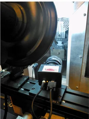
Figure 4-1: ARAMIS DIC set up on Arcan fixture tests inside heat chamber using an Instron 3382 tension machine.

The DIC apparatus which has been used for these series of experiments is the ARAMIS model 2M. ARAMIS is equipped with two 2 megapixel cameras which are able to capture 3D picture of the specimen. The system was developed by GOM mbH

(33)

24

of Braunschweig, in Germany, and is distributed by Trillion Systems in North America.

4.2. Features

The main features that put DIC towards traditional strain gauges or LVDT, [41], are:

 Full field measurements,

 No contact with the specimen,

 No limits in strain dimensions (105 µε),

 Wide range of data in one measurement: o Ux, Uy, Uz,

o

ε

x

,

ε

y

,

ε

xy(engineering strain),

 Fast test repeatability,

 Different materials TCE do not affect adhesive measurements,

 Camera calibration does not have to be carried out on site. Other relevant properties are summarized in Table 4-1.

Table 4-1: Aramis properties, [42]

ARAMIS 2 M Test campaign Camera resolution [px] 1600x1200

Standard measuring volume [mm] 10 x 7.5 to 2000x1500 30 x 24

Shutter time [ms] _{0.1 - 2000} ₁₅ Strain measuring range [%] _{0.01 up to >100} _{0.02 - 3} Strain accuracy1 [%] _0.02 _0.01 Displacement accuracy [] _{1/25 pixel} _0.7 Facet width [px] _{10 to 100} _13-15 Facet overlap [px] _{2 less than facet width} _11-13

1_{Accuracy measured for Room Temperature tests. In the ones involving heat chamber at 150 ºF strain}

(34)

25

4.3. Theoretical process, [43]

The DIC method can be resumed in 5 steps, [44]:

1) Calibration and image acquisition, 2) Subset shape function, 3) Grey level interpolation, 4) Subset correlation, 5) Post processing.

While only the first includes the whole measuring time, the other are all computational work run by the software ARAMIS.

Calibration: This is the process by which the software orients and scales the camera images to ensure the dimensional consistency of the measuring system. A 2D calibration (1 camera) is computationally easier than 3D (2 cameras), because misses the step of relating the cameras one to each other. During this phase some parameters like sensor center point, lens focal length, lens distortions and camera skew are defined.

(35)

26

Subset (facets) shape function: The DIC software divides the masked region of interest of Field Of View into many facets, the center point of each of them will give a measurement point. From the reference image to the deformed n stage, the subset shape will deform, so a mathematical function is needed to adapt this change in shape: the shape function. Most of the applications will require a rigid body movement or a warping in order to superpose the facet to its deformed region: the linear affine shape function fits the task and is computationally efficient (Figure 4-3). When linearity does not fit the deformation, a solution can be the reduction in facet size increasing as well as possible the contrast. It is then clear the affinity between it and meshing concepts in Finite Element Analysis.

Facets interpolation and matching: Interpolation is the step required to pass from a raw image data to a smoother one, which grey levels are the interpolated values of the first. It is also the (post processing) process for completing missing facets in the data. It has been found the neither linear, nor cubic-polynomial schemes work: a cubic B-spline looks the only one that can get rid acceptably of interpolation bias and noise bias along a pixel.

Once image data have been processed, facets need to be matched in subsequent images. This will involve both shape function’s deformation and interpolation information. Matching is done by minimizing a function that includes pixel intensity information, finding the best match possible for that facet. Some methods involve normalized sum-squared difference (NSSD) and normalized cross correlation (NCC).

Post processing: The commercial codes calculate the strain as a derived value, by taking the derivative of the calculated displacements which are the primary measurements. Therefore the strain data will be always noisier than the displacements. As the strain is the average in the region of the virtual strain gage, the more data points (strain length) creating the gage, the smoother the strain results.

(36)

27

Figure 4-3: Linear shape function behavior

Figure 4-4: Aramis report of a pure shear test on bonded butterfly: post processing involved filtering, interesting points and section evaluation. The strain values are in [in/in]. From the image is clear the localization and behavior of the bonded region. At this stage the load was around 4900 N (1100 lbf) and the stress on the adhesive was 18 MPa (2600 psi).

On the other hand, smoothing removes local strain gradients, then a compromise is necessary. In paragraph 4.5 are discussed the parameters that can be changed in a post processing phase for more readable results (Figure 4-4).

4.4. Experimental Process

Spraying specimen surface: In order to perform the full field measurements the system requires the specimen’s surface to have recognizable object characteristic: this means a high optical contrast needs to be achieved, and one possible way is to spray the specimen with a speckled black/white pattern (Figure 4-6). Dots size depends on field of view as pixel dimensions change: nonetheless facets are measured in pixels, that is why dots should stay around 4-7 pixels to ensure enough contrast along the gauge region (Figure 4-6). A low contrast region leads infact to higher noise data.

(37)

28

Figure 4-5: Examples of spray patterns: poor contrast (left), high contrast but not consistent (center) perfect resolution (right).

Calibration of the measuring volume: The measuring volume is the three-dimensional region where the measurement will take place and depends on the size of the measuring object or on the size of the area to be analyzed. It determines which set of lens shall be used, the measuring distance, the camera angle and base distance (3D): all of these have to be set up according to the ARAMIS setting tables provided by Trilion.

The calibration of the measuring volume provides for the use of a calibration object (panel) which is a target with a particular patter on it (Figure 4-6b). Each dot on the panel occupies more than 100 pixels, so dot centers can be interpolated up to an accuracy of 1/30 of a pixel: since the resolution is 1600x1280 the overall displacement accuracy can be conservatively stated as 1/30’000 the field of view. The pattern is memorized in the ARAMIS software and by moving manually the calibration object in the measuring space the ARAMIS software can compare the data collected with the memorized ones and determine the accuracy of the calculation itself that is expressed by the calibration deviation. For a correct calibration, the calibration deviation must be between 0.01 and 0.07 pixels.

(38)

29

Figure 4-6: Speckled pattern on D3165 (above left) and butterfly specimen (below); (b) 15x13 facets (above right) and calibration panel for small volumes ,30x24 mm2 (below right).

Illumination: Adjusting the illumination condition and consequently the shutter time is required in order to have a small camera aperture. To obtain good quality images the specimen must be illuminated with a bright light and the shutter time of the cameras must be regulated manually in relation to the quality and quantity of the illumination. The limits in this manual adjustment are a too low contrast image and, on the other hand, an overexposed one.

Noise check: After calibrating, it is a very good habit to perform a pattern check and noise floor measurements on a regular basis. This does not need to be done before every test, but it should be done before every test series. For DIC, as TRILION Systems suggests, these values are:

Displacement: Displacement noise has to be under the stated displacement accuracy2,which for this project case is 0.6 µm

2

(39)

30

Strain: Strain sensitivity does not depend on field of view.

Rule of thumb with a 1280 px is 50-100 µε (0.005-0.01 %)

A low contrast pattern, as long as a low enlightened specimen, can lead to noisy measurements. Speaking of facets, a low size facet has higher possibility to get higher noise because it includes less information on the pattern, while a wider strain length gets less noise because of the bigger averaging area (less sensibility to local effects). To check the noise, 15 images at 1/s rate were taken without moving the specimen: then three random points are picked on the surface and their values are plotted through the stages. In Figure 4-7 are showed the results coming from the room temperature noise check.

Table 4-2: Noise data at room temperature

tests recommended εx εy Ux Uy Negligible Figure 4-7: Room temperature noise check showing (a) εX, (b) Shear angle and (c) Displacement

(40)

31

Figure 4-9: Random stage points Figure 4-8: DIC creep glass door set-up.

Furthermore, before starting the creep test campaign, a check on the glass door closing the heat chamber was needed. Images were going to be taken through the door with a light on the back of the camera (to allow a smaller opening of camera aperture): even though it was made of optical glass, increase in noise could have been significant.

Taking the same allowable limits of strain and displacements given by Trylion, the results in Table 4-3 were shown by the noise check (three stage points were randomly picked, Figure

4-9). While the εx and εyare still in a good range, the displacements shown in Figure 4-11 are significantly bigger than the stated sensitivity. Nevertheless one can notice that all the 3 points undergo the same displacements which could come for possible vibrations either in the testing machine or in the door basement and result in rigid body movement. Data rearranged deleting this possible vibration show the true noise in Ux.

Table 4-3: Glass door noise check results

test recommended εx

εy

(41)

32

Figure 4-10: Normal strain εx noise level for glass door.

Figure 4-11: Aramis noise test on glass door report for displacement Ux (top). Ux data after rigid body movements correction (bottom).

(42)

33

Once having seen that the glass door did not affect measurements, a control have also been done with the functioning heat chamber. As from Figure 4-12, it can be noticed that deformation noise is consistently higher (around at least double): this is due to the hot air stream that flows from the bottom back across the chamber. Still all the positive aspects of DIC, but a lesser precision, remain intact. Nonetheless it has to be reminded that deformations are in the range of 15-20’000 µε: 300 µε represents therefore a ±2% error.

Figure 4-12: Heat chamber noise for εx and Ux. It is clear the effect of the air stream flow on the

noise measurements

After this noise measurement campaign, it was decided for a calibration with optic glass door open for measurements using the heat chamber: indeed the closing of the glass door after calibration did not give any particular change in noise as stated in Figure 4-13.

(43)

34

Initial stage: it is very important to be aware of which stage is being used as the reference stage. This will be considered having 0 strain and 0 deformation and all the measurements are differential to this reference zero condition. That is why was chosen to start taking images after having applied a preload of 133 N (30 lbf) on the specimen, that granted minimization of specimen movements due to slacks in the fixture.

4.5. Parameters, [45]

Here are listed some parameters which can be varied in order to fit the strain calculation for the particular case under investigation. This project most important boundary condition were the small dimensions of the specimen, particularly the 1 mm bond line thickness.

Spatial resolution: It is defined as the distance between independent measurement points. Increasing this value leads to a better coverage of the region of interest: this can be done decreasing facet size (typical range is 13-19 px) or decreasing facet step, which is the distance in px between left edges of adjacent facets. With facets size smaller than 11 px the accuracy decreases due to limited information for the subpixel shape fitting while a facet step smaller than half the facet size is not suitable because the measurement points are no more independent to each other.

Table 4-4: Spatial resolution parameters

Formula Current project

Pixel width [ ] _⁄ ₂₀ Data pt spacing [ ] ₂₂₀ Virtual gage length [px] _{( )}_⁄ ₂₂ Virtual gage size [ ] ₄₄₀

Maximizing this value is important for the strain calculation because it defines (decrease) the size of the virtual strain gage: the minimum strain length setting is 3 facets. It has also to be stated that a high spatial resolution leads to a higher

(44)

35

sensitivity to local strain in the data, but also to noise peaks: these can be suppressed with a median filter.

Filter: Filtering function is usually used to suppress possible noise or to emphasize local effects. When considering local strains however, engineering judgment has to be used to define if a too high spatial averaging or a filter is masking a local effect. The general rule of thumb is to filter as light as possible, however light median filtering will eliminate certain unwanted peaks. Filters parameters are runs and size (facets) of the area filtered.

It is possible to choose between 3 types of filter: 1) Average, where the statistic average of the grid is calculated; 2) Median, where the grid points values are sorted by size and the value in the middle is picked; 3) Gradient, where the gradient value set determines the max admissible slope between two grid points at which filtering is still allowed.

Displacements are always less noisy than strains, so the latter should be filtered more: for a test with relatively low strain a 2x5 and a 3x7 median, for displacement and strain respectively, can be applied. A 5x5 median filter was applied for the strain, due to the reduced spatial resolution across the bondline: infact with a 15x11 facets density there could have been 5 facets in the region of interest. Comparison between an increased run- small size (7x3) and the 5x5 median filter (Table 4-5) is showed in the images below for both a debonded stage and a pure shear stage. The differences are as expected: the small size filter worked as a smaller strain length, enhancing local effects and showing values less averaged with the neighbor facets.

Although the bonding behavior looks better enhanced with a smaller filter size, this leads to higher noise, so for more consistency in the data a 5x5 filter was chosen. To evaluate local behaviors in critical moments of load history (failure, debonding) was instead necessary to use a 7x3 one.

(45)

36

Figure 4-14: Batch 2-5, stage 50, debond region is clear in both filtered images (5x5 left, 7x3 right), but in the right one is enhanced a different load path.

Figure 4-15: Batch 3-2, stage 172, constant shear strain is more uniform with a 5x5 median filter (left).

Table 4-5: Noise check and filter summary.

Median filter type, runs x size RT, ±με Glass door, ±με 66°C, ±με

7x3 150 150 300

2x5 120 150 250

5x5 75 100 200

(46)

37

Coordinate System: As strains

ε

_x,

ε

_y,

ε

_xystrictly depend on the coordinate system, it is sometimes necessary to define a new one respect to which calculate the deformations. Indeed the specimen is not always aligned with the camera axis, leading to a misalignment of the bonded line with the y axis: this comes of particular interest for the mixed mode loading, directly giving the strain in a system orientated as the specimen. To identify a new one, only 3 points defined on the specimen (plane) surface are required.

Rigid body movement: As DIC tracks speckled pattern displacement, it is possible to get rid of the specimen rigid body movement (translation and rotation). This can be done without affecting the strain or the coordinate system, and is useful for a better visual understanding of the deformation.

(47)

38

5. EXPERIMENTAL TEST CHARACTERIZATION

5.1. Test set-up

Figure 5-1: Creep test set up: 1) Instron tension machine, 2) ARAMIS® system, 3) DIC apparatus, 4) Heat chamber with glass door, 5) Thermal controller.

All tests, both static and creep, were run using an Instron 3382 machine, equipped with load cell n° 2525-173 with a static load capacity of 100 kN (25 kip). Although the maximum load capacity exceeded by at least 30 times the maximum load applied, this did not affect at all load precision. The latter was found to oscillate about ±1 N on a held creep load of 2200 N (less than 0.1% scatter), as shown in Figure 5-2.

Thermal chamber was an ATS (Applied Test Systems) 3710, with a range of -70°C to +500°C. Its thermal controller (ATS 3000, type “T”T/C) was capable of holding 66°C with less than 0.5°C error. The chamber was equipped with an optical glass door to guarantee for correct specimen visualization.

2 1 1 5 4 3

(48)

39

Figure 5-2: Instron vibration for a held creep load of 2200 N (1/50th of maximum load).

DIC apparatus, provided by GOM and distributed by Trilion, was composed by two 50 mm lenses cameras mounted on a tripod with a led light on the back; computational post processing was completed with ARAMIS software.

5.2. Design and manufacturing

All parts involved in the testing were manufactured, treated and pre-tested at San Diego State University Department of Engineering laboratories. For Arcan fixture and butterflies are not available any standard (ASTM, ISO, DIN), therefore design was based on previous researches, which unfortunately do not provide full description of quotation and manufacturing procedure/criteria.

5.2.1. Arcan fixture

An A36 steel Arcan fixture, [4], (Figure 5-3) was fabricated for biaxial testing of Al 6061 T-651 bonded butterfly specimens, having dimensions listed in Table 5-2. There are no standards for Arcan material and shape, therefore a model was designed basing on the existing literature, [46], [47],(Figure 5-4).

(49)

40

The Arcan fixture allows changing orientation of the specimen under an uniaxial test that results in desired mixed mode loading with normal (tension/compression) and shear loading through the test region. Designed orientation allowed testing from pure shear (0) to pure tension (90) and intermediate mixed mode load conditions (22.5 and 45, Figure 5-3). The parts were machined with a water-jet cut from a steel plate.

Figure 5-3: Arcan fixture and mounted bonded butterfly.

Small dimensions of the specimen and reduced area between Arcan disks made difficult the use of traditional LVDT applied to ASTM D5656 Thick Adherend Standard Test, [33]. Also a strain gage would have been hard to handle, since it should have been as small as adhesive thickness. Non-contact full field measurements using DIC overcomes these limitations and provides accurate in-plane and out-of-plane measurements. In addition the Arcan fixture has multiple connected parts, each

(50)

41

of them having their own thermal expansions. While traditional measurement systems have to account for that to obtain true adhesive strain, by using DIC the strain was directly measured on the adhesive layer and therefore there were no issues about extraneous sources of deformation.

In Arcan fixture design, as the dimensions of the adhesive joint are quite small, particular attention has been paid to load direction misalignment, which could affect linearity of the tests.

Figure 5-4: Arcan fixture bottom side quotation, mm.

Pinned clevises were designed (Figure 5-5, Figure 5-6) to connect the Arcan fixture to the rod ends (Figure 5-7) of the load cell and so to the test platform. This minimized any additional loading on the joint due to misalignments.

(51)

42

Figure 5-5: Arcan and clevises, connected to the Instron through the rod.

(52)

43

A36 rods were designed to fit the Arcan through the height of the environmental chamber. The design concept followed the one used for the clevis, with an additional safety ring at the top for more accurate load transfer.

Figure 5-7: Steel rod design sheet, in.

5.2.2. Aluminum butterflies

Half butterflies were cut with a water-jet machine from an Aluminum 6061 T-651 plate (one of the most common aluminum alloys), and later polished to the desired dimensions. Material choice was done for its isotropic behavior (with respect to composite specimen) and material availability: indeed what mattered was to reproduce the reality of a joint (interface interactions) and not the adherend state of stress.

Butterfly specimen bonding process followed four steps: (1) Butterflies water-jet cut from Al 6061 T651 plate,

(53)

44 (2) chromic acid surface etching,

(3) two-part epoxy EA 9394 adhesive mixing and application,

(4) 3-5 days curing on a mold plate at room temperature (24°C) to fix bondline geometry.

Figure 5-8: Aluminum bonded butterfly nominal dimensions, mm. Quotations are a bit odd due to desing in imperial units.

5.2.2.1. Aluminum butterflies surface preparation

Chromic acid etching, along with phosphoric acid anodizing, are the suggested metal surface treatments in the adhesive producer guide, [48], [49]. The first creates an aluminum oxide layer (Al2O3) which is really good for its nanoscale irregular surface and hardly reacts with any other substances. Surface treating is a fundamental and very delicate step for correct adhesive/adherend interface bond, [50], as emphasized

(54)

45

by the tests: wrong surface polishing prior etching or touching etched surface could indeed lead to adhesive failure.

Table 5-1: List of devices and materials for chromic acid etching of aluminum surface

LABORATORY DEVICES CHEMICALS Glass stir rod

2 Glass beakers (1500 mL) Plastic spoon and knives Scale (0.1 g precision) Stainless steel Tong Hot plate and Oven gloves Spray bottle for DI water

D.I. water 1 lt

H2SO4 (Sulfuric Acid) 300 g Na2Cr2O7·2H2O (Sodium Dichromate) 60g 2024 Bare Aluminum (0.02 in) 1.5 g Aluminum degreaser (Trichloroethane - C2H3Cl3)

Process:

1) Degrease metal surface:

1.1. Immerse the surface inside a container with Trichloroethane 1.2. Soak for 30 sec

1.3. Rub surface with a cotton ball and let it dry 2) Set all devices in the fume hood

3) Prepare solution in a glass bowl:

3.1. Heat up to 150-160 °F ( The plate temperature has to be higher than that, as the glass container is thermally insulating)

3.2. Weigh Sodium Dichromate and solubilize in DI water 3.3. Weigh Sulfuric Acid and add to the solution

3.4. Add Aluminum to seed the bath

3.5. Mix until Al is dissolved or solution has become black

4) Use tongs to put butterflies inside solution and etch metal in bath for 12-15 min 5) For each butterfly: take out of solution, spray surface with DI water and put inside

(55)

46

6) Pour solution inside disposal container and rinse butterflies in tap water for 5 min, followed by another DI water spray

7) Display butterflies on another container to dry on the hot plate at 120-140 °F 8) Prepare two part epoxy EA9394 adhesive

8.1. Weight Part A (17-100 ratio to part B) and add the rest in part B 8.2. Mix for 3-5 min with a plastic utensil

9) Prime and bond within 16 Hr, putting adhesive on both butterfly surface before joining them on the mold

10) Remove extra epoxy on the bonding line, but not too much, better leave a bit which can always be removed through sanding than taking too much off

The curing mold was designed basing on an example found in Testing Adhesive

Joints: Best Practices, [4]. It was shaped so that 12 bonded butterflies at a time were

kept at fixed distance for the duration of the cure (Figure 5-10): mold machining provided for a precision of ±50µm in bolt hole distances, guaranteeing an adhesive thickness variation of ±5%. Excess adhesive that squeezed out was removed using a sand paper (Figure 5-9).

(56)

47

5.2.2.2. Bondline cure

Figure 5-10: Bonded butterfly curing mold, with inset showing solution used for specimen correct detaching (back of the plate).

5.3. Preliminary static tests

5.3.1. Fixture and measurement checks

During pre-test phase there was the doubt on whether to choose between 2D (one camera) and 3D (two camera) measurements. The latter were indeed considered redundant, as Arcan should have provided no out of plane displacements. Moreover using one camera would have been easier to calibrate. Unfortunately, using only one camera, measurements were really sensitive to the small (units of µm) out of plane displacements during fixture tightening under load. This led to completely wrong normal strain measurements, especially during tests under pure shear loads. The reasons of such unexpected strains were found thanks to a check, which involved using two strain gages applied to the Al region of the butterflies (one on the front and one on the back). Such test confirmed the absence of bending (which could have been

(57)

48

a possible reason for the normal strains) and emphasized the critical sensitivity of 2D measurements. Therefore all creep tests run were done using two cameras.

Figure 5-11: Pure shear load test with strain gage on Al region, positioned normal to the bond region. The specimen failed at 7120 N (26 MPa)

5.3.2. Bond area dimensions

After having being polished with sand paper every specimen bondline was measured with a digital caliper in thickness and length (Table 5-2), to assess the variation of such measures. From Table 5-3, it is clear the consistency in bond area dimensions through the different batches.

Table 5-2: Nominal dimensions of bonded butterflies, mm

Butterfly thickness

Bondline

length Bond area

Bondline thickness Bondline thickness variation Butterfly base width 12.7 20.6 260 1 ±0.1 50.8

Still from the same table, it can be noticed a slight increase in specimen bond length and a 30% increase in thickness: this was due to the re-use of previously bonded

(58)

49

butterflied for latter batches. Mechanical polishing operation, indeed, removed the very first aluminum oxide/ adhesive layer from tested specimens to create new bondable surfaces.

Table 5-3: Static test & bond area dimensions resume.

Batch 1 2 3 4 5 6 7 Number of specimen 5 8 4 4 12 11 9 Static tests 5 8 4 4 7 4 3 Creep tests3 - - - - 5 6 5 Bond Area, mm2 Average length 20.7 20.4 20.82 20.9 20.58 21.0 21.5 Avg thickness 0.9 1 1 1.1 1.4 1.5 1.45 Average width 13.0 13.2 13.05 13.1 12.9 13.18 13.0 Failure strength (avg, N) Pure shear ₆₂₀₀ _{3900 3800 3200 6200} _{4800 6300} Normal _- _- _- _{2220 5450} _{8300 5380} Mixed mode _- _- _- _- ₆₂₅₀ _- _-

Failure mode4 A A/C A A C C C

5.3.3. Static failure tests

Prior to starting creep tests, 35 bonded butterflies were tested to failure (Table 5-3) at room temperature to verify manufacturing reliability, paying particular attention to repeatability of the process and to cohesive failure. Adhesive properties obtained from such failure tests are summarized in Table 5-4 while average failure stress along with test scatter is plotted for pure shear in Figure 5-14. Summary of the static tests results can be found in Table 5-3.

3_{Sum of static and creep tests does not give batch total because of unwanted failures during handling.} 4