Optical Techniques for Experimental Tests in Microfluidics

(1)

ALMA MATER STUDIORUM – UNIVERSITÀ DI BOLOGNA

DOTTORATO DI RICERCA IN

Ingegneria Energetica, Nucleare e del Controllo

Ambientale

Ciclo XXVIII

Settore Concorsuale di afferenza: 09/C2 Settore Scientifico disciplinare: ING-IND/10

Optical techniques for experimental tests

in microfluidics

Presentata da: Giacomo Puccetti

Coordinatore Dottorato:

Chiar.mo Prof. Vincenzo Parenti Castelli

Relatore:

Chiar.mo Prof. Gian Luca Morini

Correlatore:

Dott.ssa Beatrice Pulvirenti

(2)

(3)

A tutti quelli che credono nei loro sogni. A mio padre e mia madre.

(4)

(5)

Acknowlegements

First of all, I would to express my gratitude to my supervisor Profes-sor Gian Luca Morini, who guided me during the doctoral course giving me fundamental suggestions. Thank you also for the revision of this dissertation. I am very thankful also to Dr. Beatrice Pulvirenti for all her helps, suggestions and discussions. Many thanks to Prof. Christian Kähler for the opportunity of the visiting period as a PhD student at the LRT-7 department of Fluid Mechanics and Aerodynam-ics of Universität der Bundeswehr München, Germany. I enjoyed to work on the fascinating field of Thermochromic Liquid Crystals. Special thanks to Dr. Massimiliano Rossi for his constant presence and teachings during my period in Munich and his help after it. My gratitude goes also to Dr. Pamela Vocale for all her efforts in our joined works and publications. I should like to extend my warm thanks to all the people who directly or indirectly have contributed in the achievement of the results here reported, starting from Dr. Roberta Randi and Dr. Fabrizio Tarterini for SEM images, Prof. Laura Calzà for the images with microscopy confocal fluorescence and Mr. Maurizio Chendi and Dr. Stefania Falcioni for the technical support in laboratory. I am thankful to Prof. David Newport from the Depart-ment of Mechanical, Aeronautical and Biomedical Engineering of the University of Limerick, Ireland and to Prof. Marcos Rojas-Cárdenas from the Institut Clement Ader of the University of Toulouse, France, who accepted to review this dissertation. Last but not least, I am grateful to all the people who stayed at my side during my doctoral studies, especially to my parents and my girlfriend who shared with me beautiful and difficult moments along these three years of study and research.

(6)

(7)

Abstract

This PhD dissertation deals with the use of optical, non-invasive measurement techniques for the investigation of single and two-phase flows in microchannels. Different experimental techniques are presented and the achieved results are critically discussed.

Firstly, the inverse use of the micro Particle Image Velocimetry technique for the detection of the real shape of the inner cross-section of an optical accessible microchannel is shown by putting in evidence the capability of this technique to individuate the pres-ence of singularities along the wetted perimeter of the microchan-nel. Then, the experimental measurement of the local fluid tem-perature using non-encapsulated Thermochromic Liquid Crystal particles is discussed. A deep analysis of the stability of the color of these particles when exposed to different levels of shear stress has been conducted by demonstrating that these particles can be used for simultaneous measurements of velocity and temperature in water laminar flows characterized by low Reynolds numbers (Re < 10). A preliminary experiment where the TLC thermography is coupled to the APTV method for the simultaneous measurement of the three-dimensional velocity and temperature distribution in a microchannel is shown. Finally, an experimental analysis of the different flow patterns observed for an adiabatic air-water mixture generated by means of a micro T-junction is discussed. The main air-water mixture features have been deeply observed in 195 differ-ent experimdiffer-ental conditions in which values of superficial velocity ranging between 0.01 m/s and 0.15 m/s for both the inlet flows (air and water) are imposed. The flow patterns of the air-water mixture are strongly influenced by the value of the water superficial velocity; on the contrary, the air superficial velocity plays a secondary role for the determination of the characteristics of the bubbles (i.e. length).

(8)

(9)

Sommario

La presente tesi di Dottorato è volta all’utilizzo di tecniche ottiche sperimentali non invasive per lo studio di flussi monofase e bifa-se all’interno di microcanali. Diverbifa-se tecniche sperimentali sono presentate ed i risultati ottenuti vengono discussi in maniera critica.

Inizialmente, viene mostrato l’utilizzo inverso della tecnicaµPIV per il rilevamento della reale forma della sezione di passaggio di un microcanale avente accesso ottico, mettendo inoltre in evidenza come tramite questa tecnica sia possibile individuare la presenza di singolarità geometriche lungo il perimetro bagnato della sezione. L’attenzione viene quindi rivolta all’utilizzo di particelle di Cristalli Liquidi Termocromici non incapsulati per la misura della tempe-ratura locale di un flusso liquido all’interno di un microcanale. In particolare viene analizzata la stabilità del colore riflesso da parte di queste particelle quando sottoposte a diversi valori di sforzo di taglio, dimostrandone il loro corretto impiego come tracciante per la misura contemporanea del campo di temperatura e velocità per un flusso d’acqua avente un numero di Reynolds inferiore a 10. Un espe-rimento preliminare in cui la termografia tramite TLC è accoppiata al metodo APTV per la misura simultanea del campo tridimensio-nale di temperatura e velocità viene quindi mostrato. In fine, viene presentata un’analisi sperimentale sui diversi modelli di flusso os-servati per una miscela adiabatica di aria ed acqua all’interno di una micro giunzione a T. Le principali caratteristiche della miscela bifase sono state osservate per 195 differenti condizioni sperimentali in cui la velocità superficiale delle correnti di acqua ed aria in ingresso è stata fatta variare tra 0.01 m/s e 0.15 m/s. Le caratteristiche delle bolle ed i modelli di flusso della miscela aria-acqua sono fortemente influenzati dal valore della velocità superficiale dell’acqua mentre la velocità superficiale dell’aria assume un ruolo secondario.

(10)

(11)

List of Figures

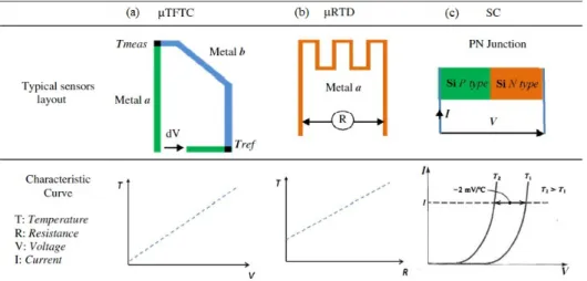
1.1 Schematic sketch of the working principle of one-dimensional MTV. 15

1.2 Simplified description of the working principle of Thin Film Ther-mocouples (a), Thin Film Resistances (b) and Semiconducting

Tem-perature sensors (c) (Morini et al.,2011). . . 21

1.3 Schematic representation of the radiative contributions recorded by the IR camera. Image adapted fromLiu and Pan(2016). . . 22

2.1 Layout of the experimental apparatus: 1) Microchannel 2) Inverted microscope 3) Laser 4) Beam-forming optics 5) Dichroic mirror 6) Objective lens 7) CCD Camera 8) Syringe containing the working fluid seeded with fluorescent particles 9) Syringe pump 10) Synchro-nization unit 11) Software unit 12) Remote laser control.(dimensions not in scale).. . . 32

2.2 Picture of the straight microchannel under investigation. . . 33

2.3 Drawing of the involved beam-forming lenses. . . 33

2.4 Picture of the involved beam-forming lenses. . . 34

2.5 The experimental apparatus. . . 35

2.6 The experimental apparatus. . . 35

2.7 Schematic sketch of the depth of correlation due to the volume illumination. . . 39

2.8 Picture of the fluorescent particles, dispersed in the working fluid, acquired in gray-scale. . . 46

2.9 Black and white picture resulting from the subtraction of the gray-scale image by the mean obtained image. . . 46

2.10 Grid made up by the interrogation cells. . . 47

(16)

2.12 Sketch of the trapezoidal cross-section of the microchannel. In the picture Nprepresents the horizontal planes and Nvthe vectors on

each row of each plane. Figure A refers to the preliminary experi-mental campaign in which 11 horizontal planes were considered. Figure B refers to the refined research in which the number of hori-zontal planes is increased up to 19. The central plane is highlighted in red for both the cases. For image clarity, the number of vectors nvis reduced in both the figures.Φ are the angles under investigation. 50

2.13 Schematic representation of the three indexes associated to the vector map. . . 51

2.14 Schematic representation of the methodology adopted. . . 52

2.15 Results for the squared straight channel forΦ angles of 90° (A,B,C), 88 (D,E,F)° and 86° (G,H,I). . . 53

2.16 Enlargement of fig.2.15E. . . 54

2.17 Picture of the microchannel under investigation: the two horizontal shaded lines are the lateral boundaries of the channel. . . 57

2.18 Results for the squared straight channel forΦ angles of 88° over 15 of 19 planes. . . 58

2.19 Reconstruction of the three-dimensional velocity distribution real-ized by collecting together all the bi-dimensional velocity data in each plane. . . 59

2.20 Error map obtained from the comparison between experimental velocity points and ones obtained with a numerical simulation in which a trapezoidal shape withΦ angles of 88° is assumed as the geometry of the microchannel cross-section. . . 60

2.21 SEM image with a magnification of 800 ×. . . 61

2.22 SEM image with references. . . 62

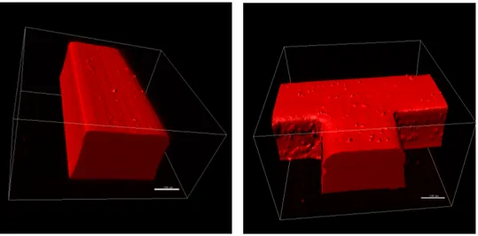
2.23 Reconstruction of the three-dimensional shape of the fluorescent fluid. . . 64

2.24 Reconstruction of the three-dimensional shape of the fluorescent fluid with references . . . 65

2.25 Sketch of the trapezoidal section with references. . . 66

2.26 Different configurations utilized for theµPIV measurements inside the micro T-junction. . . 67

2.27 Vector map of the experimental velocity distribution for the config-uration 1 with references. . . 68

2.28 Vector map of the experimental velocity distribution for the config-uration 2 with references. . . 68

2.29 Comparison between experimental and numerical data for the configuration 1. The different positions refer to the image depicted in fig.2.27. . . 69

2.30 Comparison between experimental and numerical data for the configuration 2. The different positions refer to the image depicted in fig.2.28. . . 70

(17)

LIST OF FIGURES xiii

3.1 Schematic representation of phase transitions typical of thermochromic liquid crystals (Image adapted fromHallcrest LCR(2014)). . . 77

3.2 TLC in a smectic phase. . . 78

3.3 TLC in the nematic phase. . . 78

3.4 Thermochromic liquid crystal structure in the cholesteric phase. p is the pitch of the helical path. . . 79

3.5 Example of the color play shined from non-encapsulated TLCs particles (made with Hallcrest bulk material "R20C10W"). . . 80

3.6 Non-encapsulated TLC particles at a fixed temperature (20.2 °C) inside a microchannel: the suspended flowing particles are marked by the circles with an arrow while stuck particles are marked from the gray dotted circles. The top right box shows a zoom of a TLC particle in which both the real edge of the particle and its central core are visible. As it is shown from the inset, only the central core of the particle reflects light depending on its temperature, while the peripheral area is almost transparent. . . 85

3.7 Experimental test rig layout.(dimensions not in scale). . . 87

3.8 Bottom view (A) and top view (B) of the microchannel carved into the copper substrate and sealed to a microscope slide. In the picture B is visible the hole carved into the copper substrate for housing the mini Pt1000. . . 88

3.9 Picture of the coupling between the microchannel and the Peltier heating device. . . 89

3.10 Front picture of the experimental apparatus. . . 90

3.11 Rear picture of the experimental apparatus. . . 90

3.12 Non-encapsulated TLC particles (Hallcrest UNR25C5W ) at 20.6 °C. 91

3.13 Non-encapsulated TLC particles (Hallcrest UNR25C5W ) at 22.2 °C. 91

3.14 Relative velocity between a spherical particle and an unperturbed shear flow, (A) for a particle that follows faithfully the flow and (B) for a particle stuck to a surface. . . 93

3.15 On the left: Sketch of a longitudinal section of the microchannel. In the blue box a sketch of a TLC particle stuck to the bottom wall exposed to the flow. On the right: Distribution of shear rate at the bottom wall for an unperturbed flow at Re=7.5. . . 95

3.16 Color shined by non-encapsulated TLC particles at different tem-perature when no shear flow is imposed on them. In the row A) particles with a color range of 5 K (Hallcrest R20C5W ) while in row B) particles with a color range of 10 K (Hallcrest R20C10W ). . . . 96

3.17 Image of a single non-encapsulated TLC particle (∆T=10K) exposed to different wall shear rate for different values of imposed tempera-ture. . . 97

(18)

3.18 Temperature response as a function of the average wall shear rate for TLCs with∆T = 10 K (A),∆T=5K (B) and∆T=1K (C). The con-tinuous line represent the average temperature imposed by the Peltier element and the dashed lines represent the uncertainty of the thermal control. . . 98

3.19 Difference between the mean measured temperatures (dots) and the temperature imposed by the Peltier device normalized with the temperature working range of 10 K. . . 99

3.20 Difference between the mean measured temperatures (dots) and the temperature imposed by the Peltier device normalized with the temperature working range of 5 K. . . .100

3.21 Difference between the mean measured temperatures (dots) and the temperature imposed by the Peltier device normalized with the temperature working range of 1 K. . . .100

3.22 Pictures of particles stuck to the glass bottom wall of the microchan-nel under different flow rate conditions of the working fluid: specifi-cally, in the picture B the flow rate is higher than in picture A. In the figure are shown all the effects related to the flowing of the working fluid on the particles stuck to the wall. The destruction of a particle is highlighted inside the yellow circle, while the red arrow marks the spreading of the TLC material on the glass wall. In the green box is possible to see the particles’ detachment when the flow rate of the working fluid is increased. . . .102

3.23 Destroyed non-encapsulated TLC particles (%) depending on the wall shear rate. The dotted line corresponds to wall shear rate of 400 s-1. . . .103

3.24 Layout of the experimental apparatus for the TLC temperature measurements with the addition of the cylindrical lens. . . .104

3.25 Schematic sketch of the working principle of particles’ defocusing in the APTV method. Image adapted fromSegura(2014). . . .105

3.26 Astigmatic images of the non-encapsulated TLC particles used for the simultaneous measurement of 3D temperature and velocity field in the microchannel. . . .107

3.27 Trend of the bulk temperature Tb(x) in the streamwise direction for

a microchannel with three wall heated at a constant temperature. .108

3.28 Simultaneous three-dimensional measurement of the temperature and velocity field for a flow in microchannel with a three walls heated at a constant temperature. . . .109

3.29 Picture of the new channel under study: the heating zone represents the zone where the flexible heater will be placed (Puccetti et al.,2015).111

3.30 Trend of the temperature in the central point of the channel cross-section, for devices realized in aluminum and copper, in steady state conditions. . . .115

(19)

LIST OF FIGURES xv

3.31 Trend of the temperature in the central point of the channel cross-section, for a device realized PMMA, for different values of flexible heater power, in steady state condition. . . .116

3.32 Trend of the temperature in the central point of the channel cross-section as function of time, for a device realized PMMA and a ther-mal power of the flexible heater equal to 0.08 W. . . .118

3.33 Flexible electrical heater. . . .119

4.1 Classification of typical two-phase flow patterns observed in mi-crochannels. The image is adapted from (Shao et al.,2009). . . .125

4.2 Example of air/water flow patterns observed in literature for an air-water mixture inside a micro mixer: in orange are drawn the flow pattern transitions found byHassan et al.(2005), with dotted green lines the transitions observed byChung and Kawaji(2004). The highlighted area represents the region under investigation in this work. The image is adapted fromShao et al.(2009). . . .127

4.3 Layout of the experimental apparatus: 1) Microchannel 2) Inverted microscope 3) Mercury lamp 4) Objective lens 5) High-speed Cam-era 6) Software unit 7) Supplementary LCD monitor 8) Water system supply 9) Air system supply 10) Shut-off valve 11) Differential gauge pressure 12) Signal amplifier 13) Multimeter 14) Analog Input Mod-ule 15) Software unit.(dimensions not in scale) . . . .128

4.4 Picture of the microchannel mounted on the inverted microscope. In the picture are reported the inlet flows of water and air, as well as, the outlet branch. . . .129

4.5 Picture of the differential pressure gauge connected to the air inlet branch. In the picture are also highlighted the shut-off valve con-nected to the pressure measurement system and the outlet reservoir.130

4.6 Picture of the entire experimental apparatus. . . .131

4.7 Detailed view of the experimental apparatus. . . .131

4.8 Pressure trend during the phase of air charge for UW= 0.13 m/s and

UA= 0.12 m/s. . . .133

4.9 Mixing zone of the T-junction at different frames: the air flow (white flow) enters from the top vertical branch while the water flow enters from the left horizontal branch (water flow is transparent). The right branch is the branch of the outlet flow. . . .134

4.10 Bubble along the outlet branch detected in more than one frame. .136

4.11 Bubble along the outlet branch detected in one frame. . . .136

4.12 Raw images of the detected front and back sides of a bubble belong-ing to the "Middle Taylor" flow pattern. . . .137

(20)

4.13 Conversion of the images from a grayscale into a black and white images. A) A threshold filter was applied in order to convert light gray pixels into white pixels and dark gray pixels into black pixels. B) A segmentation filter was later applied in order to fill the white area through the conversion of the black pixels into white pixels. . .139

4.14 Final image of a bubble with lines drawn in correspondence of its contours: in red is detected the inner core of the bubble, while in yellow the outer shape. . . .140

4.15 Experimental flow pattern map observed. In light green the area of superficial flow velocities in which the Short Taylor regime has been observed, in light yellow the one belonging to Middle Taylor regimes, in orange is outlined the Long Taylor regimes and finally in light purple the Taylor-Annular regime. . . .143

4.16 Example of bubbles belonging to the four different flow patterns ob-served, obtained by merging different frames. For clarity of image, some frames are skipped in the reconstruction of "Long Taylor" and Taylor-Annular bubbles. . . .144

4.17 Velocity of the bubbles for the different flow patterns as a function of the sum of superficial velocities of air and water. . . .146

4.18 Relationship between the length of the bubbles and the superficial velocity of the water for some points belonging to each flow pattern condition. (0.02 m/s ≤ UA≤ 0.15 m/s) In blue is drawn the fitting. .146

4.19 Void fraction determined experimentally as a function of the super-ficial velocity of water. . . .147

4.20 Time-averaged volumetric void fraction as a function of the homo-geneous void fraction. . . .147

4.21 Relationship between the static pressure along the branch of the inlet air supply and the sum of the superficial velocities of the wa-ter and air flows for some points belonging to different flow rate conditions. In blue is drawn the fitting line of the same. . . .148

4.22 Water droplet in silicone oil during the instant of break up. . . .151

4.23 Complete detection of a water droplet in silicone oil. . . .151

A.1 Picture of threads of fluorescent particles diluted into the working fluid after a long resting time. . . .159

A.2 Objectives used in chapter2and4. . . .159

A.3 Picture of the thermochromic liquid crystals stored inside a syringe. From this picture is clearly visible the turbidity of the liquid crystals’ material when it is in its smectic phase. . . .160

(21)

LIST OF FIGURES xvii

A.4 On the left Picture of the microchannel realized in a copper sub-strate and coupled with a Peltier device. The microchannel is housed in a raised mounting plate due to the insertion of the filter under the objective lens. The objective lens (M = 20× NA = 0.4) cou-pled with the filtering system (linear glass polarizer and achromatic quarter wave plate) is shown on the right. . . .160

(22)

(23)

List of Tables

1.1 Summary of the experimental techniques for geometry detection. . 9

1.2 Summary of the experimental techniques for velocity detection. . . 17

1.3 Summary of the experimental techniques for the fluid temperature detection. . . 26

2.1 Characteristics of the main components of the experimental test-rig. 36

2.2 Diffraction size of a point-wise light source in relation to the optical characteristics, in the last column are reported the results for the objective lens employed in the present experimental apparatus for aλ= 560 nm. . . 37

2.3 Actual diameter dimension (de/M ) of the image of a fluorescent

particle with a diameter of dpin relation to the optical

characteris-tics, in the last column are reported the results for the objective lens employed in the present experimental apparatus. The dimensions are inµm. . . 38

2.4 Depth of correlation as a function of different diameters of fluores-cent particles and optical characteristics of the objective lens. The wavelength of the light emitted from the particles is set equal to 560 nm, the objective lenses with magnification of 10 × and 20 × are supposed to be immersed in air, while the lens with M = 60 × is taken as an oil immersion lens (n0= 1.51). In the last column are

reported the results for the objective lens employed in the present experimental apparatus. The dimensions are inµm. . . 41

2.5 Characteristics of fluorescent particles and seeding concentration used in tests. . . 44

2.6 NRMS error²npfor each plane under investigation and resulting ¯²

error as a function of the inner geometry of the microchannel. . . . 55

2.7 NRMS error²np between the experimental results and a theoretical

trapezoidal shape withΦ angels of 88°, over 19 different planes along the depth of the channel. . . 57

2.8 Comparison between nominal, predicted and real values of the microchannel cross-section. . . 62

(24)

2.10 Measurements of the actual depth of the three branches at the junction. . . 65

2.11 Results for the three branches of the micro T-junction. . . 66

2.12 Calculation of theΦ angles of the straight branch. . . 67

2.13 Calculation of theΦ angles of the branches close to the junction. . . 67

3.1 Summary table of the principal components of the experimental setup. . . 92

3.2 Main properties of the PMMA used during the simulations. . . .116

3.3 Maximum Temperature of fluid flow as function of different values of the imposed heat flux Q at the wall both for a non-uniform distri-bution and for uniform distridistri-butions of the convective heat transfer coefficient h on the external surface of the device. . . .117

4.1 Summary table of the principal components of the experimental setup. . . .132

4.2 Range of superficial velocity of air and water for which the different flow patterns are established and average values of bubbles velocity for the different flow patterns in the reported range of superficial velocities and measured void fractionα. . . .145

4.3 Averaged values of the length of the bubbles and dimensionless length of the bubbles over the range of superficial velocity of water and air analyzed for each flow regime. . . .145

(25)

Nomenclature

Roman Letters

A Area (m2)

c Volume (_µl)

C Concentration (ppm)

cp Specific heat at constant pressure (J/kgK)

Ca Capillary number (-)

d Thickness / Diameter (m)

Dh Hydraulic diameter (m)

F Focal plane (-)

h Depth (m)

Convective heat transfer coefficient (W/m2K )

k Thermal Conductivity (W/mK)

L, l Length (m)

˙

m Mass flow rate (kg/s)

N Number of (-) n Refractive index (-) Particles number (-/ml) Nu Nusselt number (-) P, p Pressure (Pa) P Heated perimeter (m) p Helical pitch (m) Pr Prandtl number (-)

Q Volumetric flow rate (m3/s)

Heat power (W) Ra Rayleigh number (-) Re Reynolds number (-) S, s Displacement (m) T Temperature (K) t Time (s) u, v Velocity components (m/s) V Dimensionless velocity (-) W Average velocity (m/s) w Width (m)

(26)

Greek Letters

α Volumetric void fraction (-)

β Aspect ratio (-)

Homogeneous void fraction (-) Thermal expansion coefficient (1/K) ˙ γ Shear rate (s−1) δ Differential length (m) ε Threshold parameter (-) Uncertainty value (-) Error (-) λ Wavelength (µm, nm) µ Dynamic viscosity (kg/ms) ν Kinematic viscosity (m2/s) ρ Density (kg/m3) σ Surface tension (N/m) τ Time (s)

Shear stress (Pa)

Φ Angle (°)

Subscripts

* dimensionless

¯ average

Subscripts

0 concerning the medium in which the lens is immersed orthogonal to molecular long axis

at x = 0 A air Al aluminum B bubble b bulk c back Cu copper

e parallel to molecular long axis

em emission

ex excitation

ext external

f front

(27)

xxiii Subscripts G gas g glass in inner L liquid max maximum p particle horizontal plane pix pixel s solid surface sol solution tot total v vector

x,y,z Cartesian coordinate

W,w water w wall Acronyms 2D Two-dimensional 3D Three-dimensional µ micro

µPIV Micro Particle Image Velocimetry

APTV Astigmatism Particle Tracking Velocimetry CCD Charged-Coupled Device

CG Cover Glass (thickness)

CMOS Complementary Metal-Oxide Semiconductor DeLIF Dual emission Laser Induced Fluorescence DOC Depth Of Correlation

HSI Hue, Saturation, Intensity

IR Infra Red

LC Liquid Crystal

LDV Laser Doppler Velocimetry LIF Laser Induced Fluorescence

LIFPA Laser Induced Fluorescence Photobleaching Anemometry

M Magnification

MTT Molecular Tagging Thermometry MTV Molecular Tagging Velocimetry

NA Numerical Aperture

(28)

PIV Particle Image Velocimetry PMMA Poly(Methyl Methacrylate)

POD Proper Orthogonal Decomposition PSV Particle Streak Velocimetry

PTV Particle Tracking Velocimetry RGB Red Green Blue

RTD Resistance Temperature Detector SC Semi-Conductive Sensor

SEM Scanning Electron Microscopy SIV Scalar Image Velocimetry TFTC Thin Film Thermocouple TLC Thermochromic Liquid Crystal UV Ultra Violet

(29)

Introduction

Microfluidics is an interdisciplinary field devoted to the study of the manipulation and control of small amount of fluids (from milliliters to pico-liters) flowing in systems having dimensions ranging from tens to hundreds of micrometers for single phase flows (Kandlikar and Grande,2003;Tabeling,2005;Whitesides,

2006;Kandlikar,2012) and up to millimeters for two-phase flows (Serizawa et al.,

2002;Mehendale et al.,2000;Kandlikar et al.,2013). In these microsystems the

features of convective flows can deviate from the well known behavior observed for flows in conventional systems. In fact, when the system dimensions are reduced to the microscale, the surface forces become predominant over volume forces and this fact determines a change on the basic transport phenomena

(Tabeling,2005;Bruus,2008). The huge interest on the analysis of single phase

and two-phase convective flows through microchannels have determined an increasing number of microfluidics applications in many fields, spacing from biomedical applications to the technological field (Abgrall and Gué,2007;Kumar

et al.,2011).

Drug delivery (Saltzman and Olbricht,2002;Goettsche et al.,2005), DNA ma-nipulation (Wong et al.,2003), detection of antigens for immunological analysis

(Bessette et al.,2007;Chen et al.,2011) and detection of cancer cells with related

treatment (Chen et al.,2012;Khan et al.,2013) are just some examples of fields in which microfluidic devices found currently employment for bio-medical applica-tions. Additionally, direct applications of microfluidic systems on patients can be possible, as described in the work ofZiaie et al.(2004), in which, the authors present different techniques for the machining of bio-compatible micro devices. The authors, furthermore, draw the attention to the microfluidic hydrogel sys-tems for the detection of the glucose and to the application of these syssys-tems as integrated devices for the insulin delivery to patients affected by diabetes.

As described byYager et al.(2006), due to the overall dimensions of the mi-crofluidics devices coupled with their availability for specific diagnostics (the so called lab-on-a-chip) without an employment of heavy and bulky instrumenta-tion, lab-on-a-chip devices can be regarded as a personal points of care which anybody can hold in his own home, like glucose detectors, or, for more complex devices, can find also in small doctor’s offices rather than going in large special-ized clinics (Altieri and Camarca,2001;Jones and Meier,2004;Nichols,2007).

(30)

microfluidic devices will be affordable also for the countries historically poor, the lab-on-a-chip systems will have a large distribution with a greater impact all over the world.

Not only biomedical applications have been developed in these last decades. In microchannels, the surface-to-volume ratio between the channel surface in which the fluids flow and its volume, increases. Thus, all the forces that scale with the surface become more important than the volume forces. Therefore heat and mass transfer can be enhanced in microfluidic systems both in presence of two-phase and single phase flows because these devices are characterized by large exchange surfaces combined with limited volumes (ultra compact ex-changers) (Tabeling,2005;Kumar et al.,2011). As a consequence of these features microfluidic devices, such as, micro heads of inkjet printers (Meinhart and Zhang,

2000), micro pumps (Yoshida,2005), micro heat exchangers (Mehendale et al.,

2000;Morini,2004;Brandner et al.,2007), micro mixers (Lee et al.,2011), micro

reactors (Kumar et al.,2011) and micro systems for cooling of electronic devices

(Kandlikar et al.,2013) are currently applied in several industrial fields.

As always happens for all the new technologies, in order to further develop them and to enhance their effectiveness and reliability, the availability of sup-porting experimental data and numerical models become essentials. However, in microfluidics, due to the small dimensions of the devices, in order to limit the disturbance of the measurements on the flow, direct experimental measurements on flow characteristics (i.e. velocity and temperature distributions) can be only achieved using sensors placed on the surface of the microchannel or through the employment of a dispersion of particular tracers having micron and sub-micron dimensions. In this case the estimation of the flow features is then shifted to the evaluation of the properties and/or the motion of these tracers within the fluid. In many cases, nevertheless, the only experimental raw data are not sufficient to have accurate information about local characteristics of the transport phenom-ena, since the small dimensions of the devices inhibit the possibility to obtain a complete set of experimental data. In fact, direct observations are not everywhere possible due to the impossibility to access to some particular regions or due to shadowing effects linked to the presence of obstructions, fittings, walls and so on. Therefore the complete analysis of the flow behavior inside a microchannel can be regarded as an assimilation of gappy data. In these conditions, it becomes mandatory to couple numerical simulations to experimental tests in order to retrieve the desired information as observed byMorini and Yang(2013). In partic-ular in these cases, the set of measurement data are used as boundary conditions for the solution of the numerical problems in order to reconstruct the fluid fea-tures within the whole microdevice; in this sense, inverse techniques (Özisik and

Orlande,2000) can be efficiently employed with this aim in microfluidics.

Inverse techniques and data assimilation are concepts widely used from quite a long time for the analysis of the systems that are too broad to be accurately experimentally evaluated in each part of them. Assimilation data analysis were routinely employed in meteorology (Derber,1989;Stauffer and Seaman,1994;

(31)

3

Bouttier and Courtier,2002), oceanography (Robinson and Lermusiaux,2000)

and heart science (Reichle,2008). The idea to merge numerical models with experimental observations and to use their coupling to refine the set of data by deducing information related to the regions not directly monitored or erro-neously observed, has been applied also in fluid dynamics (Gunes et al.,2006;

Raben et al.,2012;de Baar et al.,2014) with the aim to demonstrate that

numeri-cal simulations can integrate the set of experimental measurements within the fluid region. As an example, specific gappy data methodologies based on the use of proper orthogonal decomposition (POD) (Venturi and Karniadakis,2004;

Venturi,2006) or Kriging interpolation (Gunes et al.,2006) have been proposed

in order to reconstruct the velocity field of a flow around and past a cylinder. In particular these methodologies were analyzed by the aforementioned authors for an increasing level of missing data. The missing data were artificially generated by the authors by removing simulated results in random positions within the flow region. For all the missing levels of data,Venturi and Karniadakis(2004) and

Gunes et al.(2006) demonstrated that the gappy data methodologies are able

to recover the erased data with excellent efficiency. More recently,Raben et al.

(2012), adopted an adaptive gappy POD in order to replace and reconstruct the erroneous data obtained via experimental PIV measurements of a water turbulent flow along a vertical channel. Also in this work, to demonstrate the reliability of the methodology, missing data in correspondence of erroneous measurements were obtained through a randomly removal of some experimental data. The authors showed in conclusion as the reconstructed velocity field was in good agreement with the original one.de Baar et al.(2014) used a Kriging interpola-tion of stereoscopic PIV observainterpola-tions in order to refine the data acquired over 12 planes in which the measurements of the three dimensional velocity field generated by a micro air vehicle were taken. Through the Kriging interpolation the authors were able to reconstruct the data over intermediate planes in way to decrease the space between the measurements. In order to evaluate the re-constructed data, the authors made PIV observations in correspondence to the fictitious planes and compared those experimental observations with the recon-structed data. A qualitative good agreement was found byde Baar et al.(2014) between the data generated through the Kriging interpolation and the observed data which confirms that assimilation data can be very useful in all the situations in which a complete set of experimental data becomes impossible to obtain due to big (or small) dimensions of the system: in this sense, microfluidics presents similar problems to extended systems like the oceans, atmospheric regions and so on. In addition, when the experimental data are used as starting point for the deduction of the behavior of the flow in regions not monitored directly, the accuracy of the experimental data becomes crucial in order to perform a cor-rect reconstruction of the trend of the physical quantities in the areas in which these quantities were not observed. Even though these considerations can be considered valid in general, for microfluidics applications the accuracy of the experimental data becomes more and more important.

(32)

In microfluidics, even very trivial boundary conditions, like the correct knowl-edge of the cross-section geometry of a channel can be problematic to be mea-sured and this can determine a non negligible influence on the interpretation of the measured quantities which can lead to a misunderstanding about achieved results (Shao et al.,2009;Kumar et al.,2011;Morini et al.,2011). For this reason, the proper understanding of the surrounding conditions, such as the shape and dimension of the microchannel coupled with the boundary conditions imposed to the flow, becomes an extremely important issue to keep under control in or-der to give to the experimental data the correct meaning. However, for some of these conditions there are cases in which it is not possible to perform a direct evaluation of them, as for the inner geometry of a commercial microchannel. Commercial microchannels have usually closed boundaries and therefore it is not possible to perform an accurate direct optical evaluation (i.e. SEM analysis) of their cross-section without destroying the microdevice. Hence, in order to avoid the destruction of the channel, the evaluation of the shape and dimensions of the inner geometry of the microchannel can be an example of application of inverse techniques in microfluidics in which, for example,µPIV measurements can be used in order to reconstruct the geometry of the channel as shown in the second Chapter of this dissertation.

Similarly, the direct experimental determination of the fluid temperature inside a microchannel is also a critical issue, since the dimensions of common temperature detectors are larger or at most comparable with the dimension of the inner cross-section of a microchannel. Hence, with these devices, reliable results are achievable only for temperature measurements on the channel sur-face. To overcome this problem, efforts have been made from several research groups in order to develop suitable techniques able to measure directly the fluid temperature. However, none of them can be actually considered better than others and their application is restricted to particular flow conditions, such as, a limited working temperature, or still present high uncertainties as in the case of IR thermography. One of the most promising temperature measurement tech-nique useful for microfluidics applications is the TLC thermography based on non-encapsulated TLC particles. Nevertheless, the employment of unsealed TLC particles as particle tracers in velocimetry technique like PIV, APTV and so on, has not been completely investigated up to now and in particular, no experimental results on their mechanical stability when exposed to large shear stress have been yet reported. For this reason, in the third Chapter of this dissertation, the experi-mental technique for temperature measurements based on TLCs thermography is presented and detailed information about the behavior of non-encapsulated TLCs exposed to increasing shear rates are provided.

More in detail, this dissertation is focused on the use of optical, non invasive measurement techniques for the investigation in microchannels of local velocity and temperature distribution of single phase flows and for the flow patterns obtained in presence of two-phase flows. First of all, in order to summarizes

(33)

5

the state of art of the different experimental techniques currently employed for measuring the microchannel dimensions, as well as the velocity and the temper-ature distribution of a flow inside a microchannel, a review on these techniques is presented in the first Chapter. Then, three different experimental techniques for optical investigations in microfluidics are presented and critically discussed. For each experimental technique the test rig utilized and the procedure involved are illustrated and the main results achieved are described.

In the second Chapter, the inner cross-section of a microchannel is reconstructed by using a series of velocity data observed experimentally for a liquid flow in laminar regime through a straight microchannel. The experimental velocity dis-tribution within the channel is observed by means of the technique named micro Particle Image Velocimetry (µPIV), that is nowadays one of the most reliable technique for velocity measurements in microfluidics. Firstly, the experimental data acquisition and how they can be employed for the inverse determination of the inner section of the microchannel is described. Specifically, the geometry of the cross-section is obtained by minimizing the difference existing between the velocity profiles experimentally measured and the theoretical profile obtained solving the Navier-Stokes equation for a fixed cross-section geometry. In this way, µPIV is applied as an inverse technique. The results obtained with this technique are compared with observations of destructive SEM tests which confirm the ac-curacy of the results obtained.

In the third Chapter, an experimental method for measuring the local tempera-ture of a liquid flow inside microchannels is presented. The methodology relies on the use of Thermochromic Liquid Crystals (TLCs) in their non-encapsulated form. The chapter begins with an introduction about the TLCs highlighting their working principles and how the color of those particles can be properly detected and linked to the fluid local temperature (calibration procedure). Then, the pro’s and con’s concerning the non-encapsulated TLC are underlined. One of the aspects investigated in this dissertation is the behavior of the non-encapsulated TLC when exposed to different levels of shear stress. In Section3.5the experi-mental results of the sensitivity of non-encapsulated TLC particles to shear stress are reported. Two main conclusions are reached: first, the non-encapsulated TLC particles can be subjected to certain shear stress levels before starting to break down, second, TLC particles maintain their color until the shear stress is lower of the limit value at which corresponds the TLC particle destruction. Finally, a pre-liminary experiment in which non-encapsulated TLC thermography is coupled to the Astigmatism Particle Tracking Velocimetry (APTV) for the simultaneous measurement of the three-dimensional velocity and temperature distribution in a microchannel is shown.

The fourth Chapter concerns the experimental evaluation of the air bubble gen-eration inside a water flow in a microchannel. The bubble generator is a micro

(34)

T-junction realized in fused silica in which the water flow (continuous phase) is driven in the same direction of the outlet flow while the air flow (dispersed phase) is injected orthogonally to the continuous phase. Firstly, the experimental appa-ratus is presented, then the procedure of the images’ post processing, acquired with a high speed camera, is described. The post-processed images enable the evaluation of the main physical quantities related to the air water mixture, such as the velocity and the length of the bubbles and the mixture void fraction. The experiments are repeated for 265 different conditions of flow rate imposed to the incoming liquid and gaseous flows, corresponding to superficial velocities ranging between 0.005 m/s and 0.15 m/s. Finally a flow pattern map composed by 195 experimental observations is proposed.

(35)

Chapter 1

State of the art of experimental

techniques for velocity and

temperature measurements

inside microchannels

1.1 Measurements of the dimensions of microchannel

in-ner geometry

The knowledge of the microchannel geometry has a huge impact for the determi-nation of the fluid dynamic characteristics of a microflow, like pressure drops, friction factors and so on. In fact, modifications of the channel geometry in the range of microns can induce not negligible modifications on the main flow parameters (velocity gradients and pressure drops). All the detection techniques available for the analysis of the surfaces with spatial resolution in the order of 0.1 -1µm require an optical access. The most reliable technique for geometrical inves-tigation with a resolution lower than 1µm is the Scanning Electron Microscope (SEM). Even if this investigation is undoubtedly accurate (Celata et al.,2007;Tang

et al.,2007) it presents some substantial limitations. A direct optical access is

required as well as a conductive substrate is needed. If the channel material is not conductive, such as the glass, the channel has to be previously treated with the deposition of a metallic layer (usually gold). Hence, SEM analysis allow only the investigation of an uncovered surface. For this reason, SEM investigation is a powerful tool during the channel realization, if this implies a first etching on a substrate with a subsequent bounding, while it is not at all useful for the investi-gation of already bonded microchannels, as for commercial microchannels or for a different manufacturing process, as for the cylindrical microchannels. In the latest cases, indeed, only the inlet and outlet cross-section geometry can be investigated, without destroying the devices, with this technique (Morini et al.,

(36)

2011).

In order to overcome the limitations presented by SEM investigations other techniques with a lower resolution have been proposed. As an example, the con-focal fluorescence microscopy can be used in order to detect the inner geometry of a channel with optical access. In this case the channel is completely filled with a fluorescent dye and illuminated through its whole volume. Then, through the scanning of the fluorescent region it is possible to reconstruct the shape of the filling fluid and consequently, if the fluid fills completely the channel, it is possible to reconstruct the shape of the channel cross-section. An application of this technique is shown in the Section2.5.3of this dissertation in which the con-focal fluorescence microscopy is used for the determination of the cross-section microchannel geometry of a micro T-junction. Another optical technique, able to identify the cross-section geometry of a microchannel, is presented in the second Chapter of this dissertation. The working principle of the original technique proposed bySilva et al.(2009) is to use the local velocity measurements of a flow inside a microchannel (i.e. by usingµPIV or µPTV) in order to reconstruct the cross-section geometry of the microchannel in which the fluid flows. However, the geometry reconstruction obtained by this technique has a degree of accuracy strongly linked to the accuracy of the local velocity measurements achieved by the selected velocimetry technique.

For microchannels without any optical access, the average inner diameter of the channel can be evaluated from a careful estimation of the fluid flow rate through the microchannel. More precisely,Asako et al.(2005) have proposed to use a mass flow rate measurement in order to determine the average value of the inner hydraulic diameter of microchannels. The method proposed by these authors relies on the assumptions of a Poiseuille flow inside a microchannel, a constant mass flow rate along the measurement period, constant fluid properties and a known length of the microchannel. Under these assumptions it is possible to obtain an indication of the average hydraulic diameter of a set of microchan-nels from the measurements of the mass flow rate through the microchanmicrochan-nels.

Asako et al.(2005) applied this principle in order to evaluate accurately the

inner diameter of fused silica microchannels having a declared nominal inner diameter of 150µm. The evaluation of the mass flow rate was carried out by weighing the total amount of water flowing through the channels for a time period of 10 minutes. The quantity of the water evaporated during the test was also considered from the authors. In order to give a reliable estimation of the channel diameter, the measurements were repeated for different lengths of the microchannels under investigation and the mean value of the estimated diameter was assumed to be the real diameter of the microchannels.Asako et al.(2005) demonstrate that the evaluation of the average inner diameter of a tube by using this technique is affected by an uncertainty of the order of ± 0.2 µm.

Even if, the procedure shown byAsako et al.(2005) is a smart method for the integral evaluation of the inner cross-section for microchannels without optical access, it presents some substantial limitations. First of all, the value of the inner

(37)

1.1 Measurements of the dimensions of microchannel inner geometry 9

diameter determined with this technique is an average value along the whole length of the tube. In fact, the geometry of the microchannel is assumed to be regular and constant along the axial direction, hence with this technique it is impossible to evaluate possible local imperfections of a microchannel along its axial direction. In addition, this method gives an information about the hydraulic diameter of the section, that for the cases in which the geometry is not circular, it can be obtained with different cross-section shapes. (i.e. for a rectangular channel the same hydraulic diameter can be obtained with many values of the aspect ratio). This means that this techniques cannot be useful when the goal is to reconstruct exactly the real geometry of a microchannel but only when the goal is to determine the "characteristic" dimension of the channel (i.e. its hydraulic diameter). However, even if the hydraulic diameter is extensively used as reference dimension for the evaluation of fluid-dynamic behavior of laminar flows through non-circular channels both in macro and micro systems, many authors have demonstrated that alternative definitions of the characteristic length of a channel (like the squared root of the cross-section area of a channel) could allow a more appropriate scaling of the flow characteristics when the dimensions are changed (Duan and Muzychka,2007).

TheAsako et al.(2005) technique can enable to obtain also the indication of

a different "characteristic length" (as the square root area of the channel cross-section) if there is an appropriate model which link mass flow rate to pressure drop for a fixed geometry (i.e. theDuan and Muzychka(2007) model). However, in this case the "shape" of the cross-section must be known.

A summary of the experimental techniques for the cross-section geometry detection of a microchannel is reported in Table1.1.

Table 1.1: Summary of the experimental techniques for geometry detection.

Technique Specification References

SEM

Typical resolution:

ZEISS EVO SEM

5-8 nm @ 3 kV 2-3 nm @ 30 kV

Confocal Nominal length: 300µm

(-) Fluorescence Microscopy Uncertainty: ± 3-5 %

Weighting of Nominal diameter: 150µm

Asako et al.(2005) accumulated liquid volume Uncertainty: ± 0.2 µm (± 0.16 %)

(38)

1.2 Local velocity measurements

To develop a microfluidic device, experimental techniques able to detect the flow motion inside microchannels have a relevant role in order to show the flow be-havior through the channel network. Different techniques have been proposed in order to track the local velocity distribution of microflows. Generally these meth-ods are based on optical techniques that require a transparent access to the fluid

(Sinton,2004), nevertheless, less common techniques can perform velocity and

flow patterns measurements inside micro- and mini- channels having opaque walls. Examples of these techniques are nuclear magnetic resonance or magnetic resonance imaging (Powell,2008), positron emission particle tracking (Fan et al.,

2006), radiographies with neutrons and x-rays (Sakai et al.,2003) and ultrasonic pulsed Doppler velocimetry (Peters et al.,2010). However these techniques are complex, expensive and with low spatial resolution, hence their employment is not widely widespreaded as for optical techniques. For a deepened analysis of those techniques the reader can refer to the review work ofvan Dinther et al.

(2012).

As described also bySinton(2004) the main feature of the optical techniques for flows visualization, is to slightly alter the fluid composition in order to be able to detect its movement (i.e. velocity distribution) avoiding disturbance on the behavior of the original flow. A brief description of the most used optical techniques for the measurement of local velocity inside microchannels is now summarized.

1.2.1 Micro Particle Image Velocimetry (µPIV).

The micro Particle Image Velocimetry (µPIV) technique is probably the most widely used technique for local velocity measurements of a flow inside microchan-nels, as it can be evidenced by the large number of papers in which this technique has been used for measuring the local velocity in microdevices (see reviews of

Lindken et al.(2009) andLee and Kim(2009)). This technique shares the same

working principle of the macro PIV technique, i.e. the detection of the motion of tracer particles dispersed inside the working fluid. The seeding particles are chosen in order to have the same density of the working fluid in order to obtain a complete correspondence between the motion of the working fluid and the seeding without to introduce significant disturbance on the fluid motion. In this way the detection of the particles’ displacement per unit time enables directly to calculate the related flow velocity. More precisely, theµPIV technique uses the Eulerian scheme to detect particles’ displacement, therefore, does not follow the displacement of each single particle but use the mean motion of a group of particles in a small detection area called interrogation cell. The interrogation cell must be small enough in order to give a local velocity information but also large enough to contain a minimum number of particles that give substantial information. A series of images (at least two) is required in order to associate to

(39)

1.2 Local velocity measurements 11

each interrogation cell the corresponding velocity vector. Indeed, the association of a velocity vector to each cell is obtained with a cross-correlation procedure of the particles’ displacement through the acquired series of images. In order to gain the information from sub-micron particles (this is the typical dimension of the seeding used inµPIV) a magnification of the recorded images is required, therefore the sample under investigation is visualized by using an epi-fluorescent microscope in which a magnification lens is present along the light path. This entails a volumetric illumination of the flow, hence, the focal plane in which the fluorescent particles are detected is determined from the focal plane of the objective lens rather than from a thin laser sheet as happens in conventional PIV observations. For this reason, inµPIV, not only the particles that are on the objec-tive focal plane give a useful signal but also the particles that are within a fixed layer centered on the focal plane and characterized by a thickness, called depth of correlation (DOC), give back an additional signal used in the cross-correlation procedure. A deeper analysis on theµPIV system is however postponed to the second Chapter of this dissertation, in which the main features of the experimen-tal technique and all the main developments obtained to nowadays after the first works ofSantiago et al.(1998) andMeinhart et al.(1999) are discussed.

1.2.2 Micro Particle Tracking Velocimetry (µPTV).

As for theµPIV technique, also the µPTV technique uses particles dispersed inside the working fluid in order to detect the motion of the flow. However in this case a Lagrangian approach is adopted: the displacement of each single particle is tracked, in all the field of view, from different images acquired with a constant time delay. Therefore, a velocity vector is associated to the single particle dis-placement. For this reason simplified tracking methods can also be used, even if, the related uncertainties associated to the velocity measurements are higher compared to employment of cross-correlation methods utilized in theµPIV tech-nique (Cierpka and Kähler,2012). However, theµPTV technique introduces some advantages with respect to the PIV technique as underlined bySato et al.(2003);

Cierpka and Kähler(2012) andCierpka et al.(2012). First of all, a lesser number of

particles is required. This gives a drastic advantage in order to reduce the bright noise induced by particles out of focus inside the depth of correlation and this fact decreases the effects of bias errors. In addition, for flows in steady state condi-tions the spatial resolution can be increased with respect toµPIV methods. In fact, through an acquisition of a higher number of images the distance between veloc-ity vectors is reduced, where forµPIV method this is not possible since the spatial resolution is determined by the size of the interrogation cell. In addition since commonµPIV methods employ a time-average cross-correlation of acquired data, temporal variations of the fluid velocity, such as pulsating flows, cannot be detected while through tracking methodologies this becomes possible (Sato et al.,

2003). In last instance, as shown bySato et al.(2003) through spatially-averaged methods of PTV the bias errors induced by the Brownian motion of the particles

(40)

can be eliminated also for velocity measurements with time resolution. TheµPTV has been successfully applied for velocity measurement of electrokinetic-driven flows inside microchannels (Devasenathipathy et al.,2002).

1.2.3 Astigmatism Particle Tracking Velocimetry (APTV)

Recently,Cierpka et al.(2010) have developed a PTV technique for the detection of the three-dimensional velocity field of a flow inside a microchannel, in which the information given by out-of-focus particles are used in order to obtain the dis-placement of the particles along the direction perpendicular to the observation plane. This technique is called Astigmatism Particle Tracking Velocimetry (APTV) and it is simply realized by adding a cylindrical lens along the light path between the classical spherical lens of the microscope and the CCD or CMOS sensor for image acquisition (Cierpka et al.,2012;Rossi and Kähler,2014). Three funda-mental advantages are related to the APTV method: first, this technique gives fundamental information about the three-dimensional characteristics of the flow, second, it reduces sensibly the bias error induced by out-of-focus particles and third, the measurement of the three-dimensional velocity field is possible with the employment of a single camera (Cierpka et al.,2010). About this last characteristic it is possible to highlight that the 3D velocity field can be also re-constructed through stereoscopicµPIV technique as proposed byLindken et al.

(2006). However, in this case two different cameras with a tilt angle between them are required in order to acquire simultaneously the images via a stereo lens with a magnification of 1 × or 2 ×. Nevertheless, the low numerical aperture of the stereo lenses entails a large depth of correlation (60 ± 10 µm for a lens of M = 1 × and 15 ± 5 µm for a lens of M = 2 ×) reducing consequently the spatial resolution in the direction normal to the fluid flow and therefore the reliability of this technique.

More recently,Segura et al.(2015) have demonstrated the viability of the APTV method using non-encapsulated thermochromic liquid crystal (TLC) particles, in such way to perform with the employment of a single camera, simultaneous measurements of 3D velocity and temperature distribution of a fluid in microflu-idic applications. Nevertheless, the discussion about the achieved uncertainties when the APTV method is coupled with the TLC thermography is let to Section

3.7, in which simultaneous measurements of three-dimensional velocity and temperature distribution are performed for a fluid flow inside a microchannel.

1.2.4 Micro Particle Streak Velocimetry (µPSV).

µPSV employs a dispersion of a fluorescent dye inside the working fluid which gives back a bright signal after being excited from a light source. The images of the particles are acquired from a CCD camera that integrate different frames recorded with a constant time delay in a single image. In this way it is possible to visualize the fluid motion inside the microfluidic device through the streaks

(41)

1.2 Local velocity measurements 13

obtained via the fluorescent dye. Even if quantitative velocity measurements are possible withµPSV, the accuracy of the results is strongly lower compared to the accuracy achieved throughµPIV and µPTV techniques (Sinton,2004). In the past, PSV technique has been used for tracing the fluid motion either for electrokinetic flows (Taylor and Yeung,1993;McKnight et al.,2001;Oddy et al.,

2001) than for pressure driven flows (Taylor and Yeung,1993;Brody et al.,1996) inside microchannels.

1.2.5 Laser Doppler Velocimetry (LDV).

Laser Doppler Velocimetry (LDV) or Laser Doppler Anemometry (LDA) is based on the counting of the Doppler signal gave back from reflective particles when illuminated by a laser beam. Two or more laser beam are required in order to de-tect flow velocity, since the velocity of the seeding particles is determined through the evaluation of distance of the interference fringes generated by reflective par-ticles in the unit time. As for the others techniques, LDV is born for velocity determinations in conventional channels. The application of LDV to microflows is described in the technical note ofTieu et al.(1995). More recently,Onofri(2006) published a work in which a slight modification of standard LDV technique was used in order to study the velocity distribution of a flow inside a microchannel having a depth of 80µm.Onofri(2006) used three laser beams formed by splitting the beam generated by a laser diode to illuminate titanium oxide nano particles with a diameter of 0.3 - 0.7µm. The accuracy of LDV system shown byOnofri

(2006) is in the order of 5 % with respect to the measured velocity.

1.2.6 Micro Molecular Tagging Velocimetry (µMTV) and other tech-niques.

Micro Molecular Tagging Velocimetry (µMTV), and more in general molecular based techniques use luminescent molecules, such as fluorescent or phospho-rescent dye artificially dispersed or created inside the working fluid, in order to detect the fluid velocity distribution. Hence, these luminescent molecules are ac-tivated in a fixed region by a light source (lasers, halogen lamps, UV light sources, etc...) and their velocity is evaluated by measuring the molecules’ displacement in a known time interval. To be eligible forµMTV, the molecular tracers have to respect two fundamental requirements: first, in order to furnish reliable informa-tion on the fluid moinforma-tion, the forces acting on the molecules of the dye must be the same forces acting on the molecules of the fluid (Sinton,2004) and second, the life time of the luminescent molecules must be long enough to be detected in the selected time delay (Hu and Koochesfahani,2006;Koochesfahani and Nocera,

2007). Generally, as stated also byKoochesfahani and Nocera(2007), fluorescent dye give a signal with strong intensity but for a short time (1 - 10 ns) since the non-radiative decay rate is usually negligible compared to the radiative decay rate, while phosphorescent dye give a signal with a weaker intensity but for longer

(42)

time (up to the second). Hence, the proper choice of the molecular fluorescent dye depends on the typology of application in which velocity measurements are carried out and in its turn determines the kind of light excitation.

The major advantage of the MTV technique, is that molecular tracers can be successfully employed in order to track situations in which the drift motion of the seeding micro particles induced from the shear forces of the flow could compromise the correct detection of the same fluid motion, like for gaseous flows.

Paul et al.(1998), applied for the first time a photoactivatable caged-fluorescent

dye for the visualization of pressure-driven and electrokinetically-driven flow in-side a microchannel. In the specific case, the experiments were carried out inin-side fused silica capillaries with polyimide cladding having inner diameters of 75µm and 100µm. The fluorescent caged dye was premixed into a water flow and then driven inside the capillary. The fluorescence was then induced using two lasers: a UV laser beam (λ= 355 nm) was focused inside the microchannel in order to realize a laser sheet of 20µm of thickness for uncaging the dye, then a double Nd:YVO4blue laser (λ= 473 nm) was used for exciting the dye. The light emitted

by the fluorescent dye was filtered and subsequently acquired by a CCD camera. The Scalar Image Velocimetry (SIV) method developed byDahm et al.(1992) was used in order to recover the velocity information of a pressure driven flow, while the motion of electrokinetically driven flow was directly observed through the mean displacement of the fluorescent dye. Finally the authors highlighted that the achieved spatial resolution achievable with this technique can be estimated in the order of 5µm for in-plane measurements while the depth of field was about 20µm.

Maynes and Webb(2002) used a phosphorescent dye in water solution to

mea-sure the velocity inside a fused silica microchannel with an inner diameter of 705 µm. The working principle of the technique shown byMaynes and Webb(2002) (fig. 1.1) is similar to the one adopted byPaul et al.(1998) with the difference of that the dye used byMaynes and Webb(2002) was phosphorescent and not caged, hence, a single UV laser (λ= 308 nm) was used in order to excite the dye. Also in this case the exciting light was focused inside the microchannel in order to have a laser beam with a radius of approximately 20µm. A spatial resolution of 10 µm was achieved by the authors. The technique proposed byMaynes and Webb

(2002) was applied in order to evaluate the fluid velocity inside a microchannel for Reynolds numbers ranging from 600 up 5000. The comparison with the ex-pected theoretical flow velocity, has shown a particular good agreement with the experimental data obtained for Reynolds numbers below 2000.

Wang(2005) proposed a technique called Laser Induced Fluorescence Pho-tobleaching Anemometry (LIFPA) in order to measure the fluid velocity in mi-crochannels. The key point of this technique is to correlate the fluorescence intensity of the dye with the velocity of the fluid. This principle is based on the consideration that the photobleaching effect is characterized by a fluorescence intensity which decreases exponentially in time (Wang,2005).