© 2013 ACEEE
Spiking Neural Networks As Continuous-Time
Dynamical Systems: Fundamentals, Elementary
Structures And Simple Applications
Mario Salerno, Gianluca Susi, Alessandro Cristini, Yari Sanfelice, and Andrea D’Annessa.
Institute of Electronics, Rome University at Tor Vergata E-mail: [email protected]
Abstract — In this article is presented a very simple and effective analog spiking neural network simulator, realized with an event-driven method, taking into account a basic biological neuron parameter: the spike latency. Also, other fundamentals biological parameters are considered, such as subthreshold decay and refractory period. This model allows to synthesize neural groups able to carry out some substantial functions. The proposed simulator is applied to elementary structures, in which some properties and interesting applications are discussed, such as the realization of a Spiking Neural Network Classifier.
Index Terms — Neuron, Spiking Neural Network (SNN), Latency, Event-Driven, Plasticity, Threshold, Neuronal Group Selection, SNN classifier.
I. INTRODUCTION
In Spiking Neural Networks (SNN), the neural activity consists of spiking events generated by firing neurons [1], [2], [3], [4]. A basic problem to realize realistic SNN concerns the apparently random times of arrival of the synaptic signals [5], [6], [7]. Many methods have been proposed in the technical literature in order to properly desynchronizing the spike sequences; some of these consider transit delay times along axons or synapses [8], [9]. A different approach introduces the spike latency as a neuron property depending on the inner dynamics [10]. Thus, the firing effect is not instantaneous, but it occurs after a proper delay time which is different in various cases. This kind of neural networks generates apparently random time spikes sequences, since continuous delay times are introduced by a number of desynchronizing effects in the spike generation. In this work, we will suppose this kind of desynchronization as the most effective for SNN simulation. Spike latency appears as intrinsic continuous time delay. Therefore, very short sampling times should be used to carry out accurate simulations. However, as sampling times grow down, simulation processes become more time consuming, and only short spike sequences can be emulated. The use of the event-driven approach can overcome this difficulty, since continuous time delays can be used and the simulation can easily proceed to large sequence of spikes [11], [12].
The class of dynamical neural networks represents an innovative simulation paradigm, which is not a digital system, since time is considered as a continuous variable. This property presents a number of advantages. It is quite easy to
simulate very large networks, with simple and fast simulation approach [13]. In the present work, exploiting the neural properties mentioned above, are introduced very simple logical elementary structures, which can represent useful application examples of the proposed method. With the purpose to show the structures capabilities as a processing block, a SNN classifier is presented. In this way, is possible to treat many problems, that involve the use of the classic artificial neural networks, by means of spiking neural networks.The paper is organized as follows: description of some basic properties of the neuron, such as threshold and latency; simulation of the simplified model and the network structure on the basis of the previous analysis. Then, with the aim to realize some simple applications, such as the SNN classifier, some elementary structures are analyzed and discussed.
II. ASYNCHRONOUS SPIKING NEURAL NETWORKS
Many properties of neural networks can be derived from the classical Hodgkin-Huxley Model, which represents a quite complete representation of the real case [14], [15]. In this model, a neuron is characterized by proper differential equations describing the behaviour of the membrane potential Vm. Starting from the resting value Vrest, the membrane potential can vary when external excitations are received. For a significant accumulation of excitations, the neuron can cross a threshold, called Firing Threshold (FT), so that an output spike can be generated. However, the output spike is not produced immediately, but after a proper delay time called latency. Thus, the latency is the delay time between exceeding th e membr an e poten tial FT an d th e actual spike generation.This phenomenon is affected by the amplitude and width of the input stimuli and thus rich dynamics of latency can be observed, making it very interesting for the global network evolution.
The latency concept depends on the definition of the threshold level. The neuron behaviour is very sensitive with respect to small variations of the excitation current [16]. Nevertheless, in the present work, an appreciable maximum value of latency will be accepted. This value was determined by simulation and applied to establish a reference threshold point [13]. When the membrane potential becomes greater than the threshold, the latency appears as a function of Vm.Th e laten cy times make th e n etwor k spikes desynchronized, in function of the dynamics of the whole 80
© 2013 ACEEE
network. As shown in the technical literature, some other solution s can be con sider ed to accoun tin g for desynchronization effects, as, for instance, the finite time spike transmission on the synapses [8], [9], [10].A simple neural network model will be considered in this paper, in which latency times represent the basic effect to characterize the whole net dynamics.
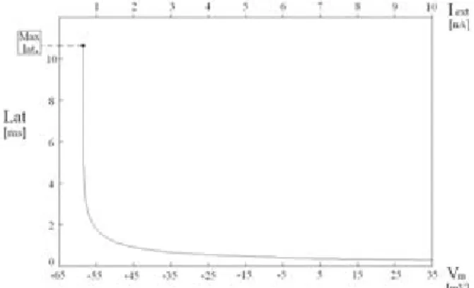
To this purpose, significant latency properties have been analysed using the NEURON Simulation Environment, a tool for quick development of realistic models for single neurons, on the basis of Hodgkin-Huxley equations [17]. Simulating a set of examples, the latency can be determined as a function of the pulse amplitude, or else of the membrane potential Vm. The latency behaviour is shown in Fig. 1, in which it appears decreasing, with an almost hyperbolic shape. These results will be used to introduce the simplified model, in the next section. Some other significant effects can easily be included in the model, as the subthreshold decay and the refractory period [10]. The consideration of these effects can be significant in the evolution of the whole network.
III. SIMPLIFIED NEURON MODEL IN VIEW OF NEURAL NETWORK
SIMULATION
In order to introduce the network simulator in which the latency effect is present, the neuron is modelled as a system characterized by a real non-negative inner state S. The state S is modified adding to it the input signals Pi (called burning signals), coming from the synaptic inputs. They consist of the product of the presynaptic weights (depending on the preceding firing neurons) and the postsynaptic weights, different for each burning neuron and for each input point [13]. Defining the normalized threshold S0 ( > 1), two different working modes are possible for each neuron (Fig. 2): a) S < S0, for the neuron in the passive mode; b) S > S0, for the neuron in the active mode.
In the passive mode, a neuron is a simple accumulator, as in the Integrate and Fire approach. Further significant effects can be considered in this case, as the subthreshold decay, by which the state S is not constant with time, but goes to zero in a linear way. To this purpose, the expression S = Sa –
Δt ld can be used, in which Sa is the previous state, Δt is the time interval and ld is the decay constant.
Fig. 1. Latency as a function of the membrane potential (or else of the current amplitude Iext , equivalently).
Fig. 2. Passive and active working modes.
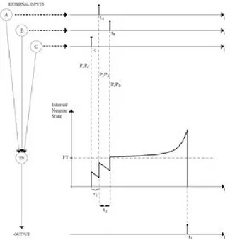
In the active mode, in order to introduce the latency effect, a real positive quantity, called time-to-fire tf, is considered. It represents the time interval in which an active neuron still remains active, before the firing event. After the time tf, the firing event occurs (Fig. 3).
Fig. 3. Proposed model for the neuron
The firing event is considered instantaneous and consists in the following steps:
a) Generation of the output signal Pr, called presynaptic weight, which is transmitted, through the output synapses, to the receiving neurons, said the burning neurons; b) Reset of the inner state S to 0, so that the neuron comes back to its passive mode.
In addition, in active mode, a bijective correspondence between the inner state S and tf is supposed, called the firing equation. In the model, a simple choice of the normalized firing equation is the following one:
tf = 1/(S - 1), for S > S0
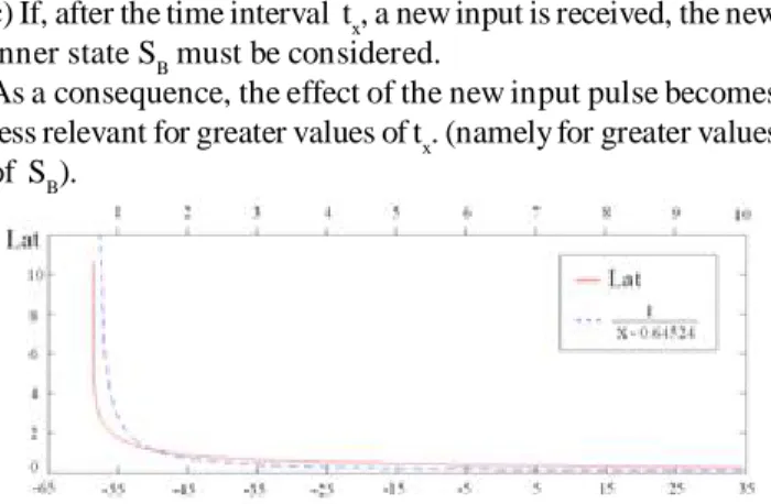
Time-to-fire tf is a measure of the latency, as it represents the time interval in which the neuron remains in the active state. If S0 = 1 + d (with d > 0), the maximum value of time-to-fire is equal to 1 / d. The above equation is a simplified model of the behaviour shown in Fig. 1. Indeed, as the latency is a function of the membrane potential, time-to-fire depends from the state S, with a similar shape, like a rectangular hyperbola. The simulated and the firing equation behaviours are compared in Fig. 4.
The following rules are then applied for the active neurons: a) If appropriate inputs are applied, the neuron can enter in its active mode, with a proper state SA and a corresponding time-to-fire: tfA = 1/(SA - 1).
b) According to the bijective firing equation, as the time increases of tx ( < tfA), the time-to-fire decreases to the value tfB = tfA – tx and the corresponding inner state SA increases to 81
© 2013 ACEEE
the new value SB = 1 + 1/ tfB.
c) If, after the time interval tx, a new input is received, the new inner state SB must be considered.
As a consequence, the effect of the new input pulse becomes less relevant for greater values of tx. (namely for greater values of SB).
Fig. 4. Comparison between the latency behaviour and that of the denormalized firing equation.The two behaviours are similar to
rectangular hyperbola.
The proposed model is similar to the original integrate-and-fire model, except for the introduction of a modulated delay for each firing event. This delay time strictly depends from the inner dynamics of the neuron. Time-to-fire and fir-ing equation are basic concepts to make asynchronous the whole neural network. Indeed, if no firing equation is intro-duced, time-to-fire is always equal to zero and any firing event is produced exactly when the state S becomes greater than S0. Thus, the network activity is not time modulated and the firing events are produced at the same time. On the other hand, if neuron activity is described on the basis of continu-ous differential equations, the simulation will be very com-plex and always based on discrete integration times.
The introduction of the continuous time-to-fire makes the evolution asynchronous and dependent on the way by which each neuron has reached its active mode.
In the classical neuromorphic models, neural networks are composed by excitatory and inhibitory neurons. The con-sideration of these two kinds of neurons is important since all the quantities involved in the process are always positive, in presence of only excitatory firing events. The inhibitory firing neurons generate negative presynaptic weights Pr, and the inner states S of the related burning neurons can become lower. For any burning neuron in the active mode, since dif-ferent values of the state S correspond to difdif-ferent tf, time-to-fire will decrease for excitatory, and increase for inhibitory events. In some particular case, it is also possible that some neuron modifies its state from active to passive mode, with-out any firing process, in the case of proper inner dynamics and proper inhibitory burning event. In conclusion, in pres-ence of both excitatory and inhibitory burning events, the following rules must be considered.
a. Passive Burning. A passive neuron still remains passive after the burning event, i.e. its inner state is always less than the threshold.
b. Passive to Active Burning. A passive neuron becomes active after the burning event, i.e. its inner state becomes greater than the threshold, and the proper time-to-fire can be evaluated. This is possible only in the case of excitatory firing events.
c.Active Burning. An active neuron affected by the burning event, still remains active, while the inner state can be increased or decreased and the time-to-fire is properly modified.
d. Active to Passive Burning. An active neuron comes back to the passive mode without firing. This is only possible in the case of inhibitory firing neurons. The inner state decreases and becomes less than the threshold. The related time-to-fire is cancelled.
The simulation program for continuous-time spiking neural networks is realized by the event driven method, in which time is a continuous quantity computed in the process. The program consists of the following steps:
1. Define the network topology, namely the burning neurons connected to each firing neuron and the related values of the postsynaptic weights.
2. Define the presynaptic weight for each excitatory and inhibitory neuron.
3. Choose the initial values for the inner states of the neurons. 4. If all the states are less than the threshold S0 no active neurons are present. Thus, the activity is not possible for all the network.
5. If this is not the case, evaluate the time-to-fire for all the active neurons. Apply the following cyclic simulation procedure:
5a. Find theneuron N0 with the minimum time-to-fire tf0. 5b. Apply a time increasing equal to tf0. According to this choice, update the inner states and the time-to-fire for all the active neurons.
5c. Firing of the neuron N0. According to this event, make N0 passive and update the states of all the directly connected burning neurons, according to the previous burning rules.
5d. Update the set of active neurons. If no active neurons are present the simulation is terminated. If this is not the case, repeat the procedure from step 5a.
In order to accounting for the presence of external sources, very simple modifications are applied to the above procedure. In particular, input signals are considered similar to firing spikes, though depending from external events. Input firing sequences are connected to some specific burning neurons through proper external synapses. Thus, the set of input burning neurons is fixed, and the external firing sequences are multiplied by proper postsynaptic weights. It is evident that the parameters of the external sources are never affected by the network evolution. Thus, in the previous procedure, when the list of active neurons and the time-to-fire are considered, this list is extended also to all the external sources. In previous works [13], the above method was applied to very large neural networks, with about 105 neurons. The set of postsyn aptic weigh ts was contin uously updated according to classical Plasticity Rules and a number of interesting global effects have been investigated, as the well known Neuronal Group Selection, introduced by Edelman [18], [19], [20], [21].In the present work, the model will be applied to small neural structures in order to realize useful logical behaviours. No plasticity rules are applied, thus the scheme and the values of presynaptic and postsynaptic 82
© 2013 ACEEE
weights will be considered as constant data. Because of the presence of the continuous time latency effect, the proposed structures seem very suitable to generate or detect continuous time spike sequences. The discussed neural structures are very simple and can easily be connected to get to more complex applications. All the proposed neural schemes have been tested by a proper MATLAB simulator.
IV. SOME BASIC DEFINITIONS AND CONFIGURATIONS
In this section, the previous theory will be applied to small group of neurons so that a number of SIMPLE continuous-time applications will be introduced. A very simple logic activity consists of the recognition of proper input spiking sequences by proper neural structures. The input sequences can differ from their spike time arrival, and the recognition consists on the firing of a proper output element, called the Target Neuron TN. A basic function called the dynamic addition will be introduced, by which many simple structures can be defined, in which the input spike time of arrival can be used.
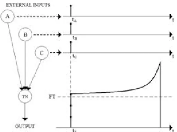
The basic function of a target neuron is to produce an output spike when the correct burning spikes are received in the proper time interval (Fig. 5). No output spike is generated if some of the inputs are not received, or else, if their arrival times are not properly correct. It is evident that the target neuron will become active under the following two conditions: 1. the sum of the burning input amplitudes is greater than the threshold.
2. the burning spikes are properly synchronized.
Fig. 5. Three input spikes are used to generate the output. The subthreshold decay effect is considered. The times τ1
and τ2 are the interspike intervals.
The subthreshold decay effect will be used as a design pa-rameter. Because of this effect, it is evident that greater input spike amplitudes are necessary, for less synchronized times of arrival (Fig. 6). In this way, the firing threshold will be reached.
Fig. 6. Comparison of different input amplitudes and arrival times, with reference to Fig. 5.
a) The inputs are quite synchronized and the output is generated.
b) The synchronization is not sufficient to output generation. c) The insufficient synchronization is compensated by proper amplitude increasing.
In order to produce the target neuron spike, the following relation must be satisfied:
Pr (Pa + Pb + Pc) – ld (τ1 + τ2) > S0
in which Pr is the presynaptic weight, Pa, Pb, Pc are the postsynaptic weights referred to the target neuron, ld is the subthreshold decay, S0 is the normalized threshold and τ1, τ2 are the interspike intervals.
The input spike time tolerance is strictly related to the subthreshold decay and to the presynaptic weight values, considered as external control parameters. On the basis of the proper choice of these parameters, a certain tolerance of the input synchronism could be obtained. Different target neuron tolerances could be achieved. Indeed, greater target neuron tolerance is observed in correspondence to greater presynaptic weights, as well as less ld values (Fig. 7). This kind of behaviour should be quite useful to synthesize higher complex structures and applications.
Fig. 7. Comparison of the target neuron behaviour as a function of different choices of ld and Pr, for a subthreshold single input spike.
a) original reference case. b) higher Pr value. c) higher ld value.
A new global useful parameter can be defined, namely the working mode activity level (WMAL). With reference to a target neuron, this parameter represents the number of equal amplitude synchronized input spikes necessary to let the target neuron over the threshold level (Fig. 8).In the previous discussion, the only considered effect was the target neuron threshold level overtaking. On the basis of the previous discussion, the actual output spike generation will occur after the proper time-to-fire, if of course other burnings will be not present in the meantime.
© 2013 ACEEE
Fig. 8. Case of WMAL equal to 3. Three equal and synchronized burning pulses are necessary. A less number of burning pulses as well
as proper desynchronization can make the output not present.
V. ELEMENTARY STRUCTURES
In this section, a number of elementary applications of the simplified neuron model will be presented. The purpose is to introduce some neural structures in order to generate or detect particular spike sequences. Since the considered neural networks can generate analog time sequences, time will be con sider ed as a con tin uous quan tity in all th e applications.Thus, very few neurons will be used and the properties of the simple networks will be very easy to describe. A. Analog Time Spike Sequence Generator
In this section, a neural structure, called neural chain, will be defined. It consists of m neurons, called N1, N2,… , Nm, connected in sequence, so that the synapses from the neuron Nk to the neuron Nk+1 is always present, with k = 1, 2, 3, … , m-1 (Fig. 9).
Fig. 9. Open neural chain.
In the figure, EI1 represents the external input, Nk the neuron k, and P(Nk, Nk-1) the product of the presynaptic and the postsynaptic weights, for the synapses from neurons N
k-1 to neuron Nk.
If all the quantities P(Nk, Nk-1) are greater than the threshold value S0 = 1 + d, any neuron will become active in presence of a single input spike from the preceding neuron in the chain. This kind of excitation mode will be called, level 1 working mode. It means that a single excitation spike is sufficient to make active the receiving neuron. If all the neurons 1, 2, .. m, are in the level 1 working mode, it is evident that the firing sequence of the neural chain can proceed from 1 to m if the external input EI1 is firing at a certain initial time. This of course is an open neural chain, but, if a further synaptic connection from neuron Nm to neuron is present, the firing sequence can repeat indefinitely and a closed neural chain is realized (Fig. 10).
The basic quantity present in the structure is the sequence of the spiking times generated in the chain. Indeed, since all the positive quantities P(Nk, Nk-1) - S0 can be chosen different with k, different latency times will be generated,
Fig. 10. Closed neural chain.
thus the spiking times can be modulated for each k with the proper choice of P(Nk, Nk-1).
In this way, a desired sequence of spiking times can be obtained. The sequence is limited for open neural chain, periodic for closed neural chain.The above elementary neural chain can be modified in many ways. A simple idea consists of substituting a neuron Nk in the chain with a proper set of neurons Nkh with h = 1, 2, … mk, (mk > 1) (Fig. 11).
Fig. 11. Extended neural chain element.
B. Spike Timing Sequence Detector
In this section, two elementary structures are discussed to detect input spike timing sequences. The properties of the structures depend on the proper choice of the values of postsynaptic weights, together with the basic effect called subthreshold decay. The idea is based on the network shown in Fig. 12. It consists of two branches connecting the External Inputs EI1 and EI2 to the output neuron TN10.
Fig. 12. Elementary Spike Timing Sequence Detector. The detection is called positive when the firing of the target neuron
is obtained, otherwise negative.
In the figure, P(10,1) is the product of the presynaptic and the postsynaptic weights for the synapses from EI1 to TN10, while P(10,2) refers to the synapses from EI2 to TN10. If the values are properly chosen, the system can work at level 2 working mode. This means that TN10 becomes active in presence of the two spikes from EI1 and EI2. As and example, if P(10,1) = P(10,2) = 0.6, and the spikes from EI1 and EI2 are produced at the same time, TN10 becomes active with the state S(TN10) = 1.2 ( > S0), so that an output spike is produced after a proper latency time. In this case, the output spike generated by TN10 stands for a positive detection. However, if the spiking times t1 and t2 of EI1 and EI2 are different (for instance t2 > t1), only the value of S(TN10) = 0.6 is present at 84
© 2013 ACEEE
the time t1. Taking into account the linear subthreshold decay, the state at the time t2 will grow down to S(TN10) = 0.6 - (t2 -t1 ) ld. Thus, the new spike from EI2 could not be able to make active the target neuron TN10; thus, the detection could be negative. This is true if the values of P(10, 1) and P(10,2), the time interval (t2 - t1) and the linear decay constant ld are properly related. In any case, the detection is still positive if the interval (t2 - t1) is properly limited. Indeed, for a fixed value of t1, the detection is positive if t2 is in the interval A, as shown in Fig. 13. Therefore, the proposed structure can be used to detect if the time t2 belong to the interval A.
Fig. 13.Symmetric interval A. When t2 belongs to interval A,the detection is positive.
The above elementary discussion can easily be extended. If the structure is modified as in Fig. 14, in which a Delay Neuron DN3 is added, the time interval A can be chosen around a time t1 +Dt, in which Dt is the delay time related to DN3
Fig. 14. Delayed Spike Timing sequence Detector.
The value of Dt can be obtained as the latency time of DN3, from a proper value of P(3,1). Of course the neuron DN3 must work at level 1 working mode.
C. Spike Timing Sequence Detector With Inhibitors In this section a structure able to detect significant input spike timing sequences will be introduced. The properties of the proposed neuron structure strictly depend on the presence of some inhibitors which make the network properties very sensitive.The proposed structure will be
described by a proper example. The scheme is shown in Fig. 15.The network consists of three branches connected to a Target Neuron. The structure can easily be extended to a greater number of branches. The neurons of Fig. 15 can be classified as follows:
TABLE I. TABLE II. TABLE III. TABLE IV.
Fig. 15. Spike timing sequence detector using inhibitors: an example. The detection is called positive when the firing of
the target neuron is obtained, otherwise negative
Table I. Firing Table For The Case A Simulation. The Detection Is Positive.
Table II. Firing Table For The Case B Simulation. No Firing For The Neuron Tn10. The Detection Is Negative.
Table III. Firing Table For The Case C Simulation. No Firing For The Neuron Tn10. The Detection Is Negative.
Table IV. Firing Table For The Case D Simulation. The Detection Is Positive.
External Inputs : neurons 35, 36, 37; Excitatory Neurons : neurons 1, 2, 3; Inhibitory Neurons : neurons 31, 32, 33; Target Neuron : neuron 10.
The network can work in different ways on the basis of the values P(k, h) of the products of the presynaptic and the postsynaptic weights.
Since the firing of the target neuron depends both on the excitators and the inhibitors, the detection can become very sensitive in function of the excitation times of the external inputs, with proper choices of the quantities P(k, h). Indeed, some target neuron excitations can make it active so that the firing can be obtained after a proper latency interval. However, if an inhibition spike is received in this interval, the target neuron can come back to the passive mode, without any output firing.
As an example, called Case A, the simulation program has been used with the following normalized values:
P(1,35) = P(2,36) = P(3,37) = 1.1; P(31,1) = P(32,2) = P(33,3) = 1.52; P(10,1) = P(10,2) = P(10,3) = 0.5; P(10,31) = P(10,32) = P(10,33) = - 4.
In this example, the three parallel branches of Fig. 15 are exactly equal and the latency time for the target neuron firing is such that the inhibition spikes are not able to stop it. In the simulation, equal firing times for the external inputs are chosen (equal to the arbitrary normalized value of 7.0000). The firing times (t) for the neurons (n) are obtained by the simulation program (Tab. I).It can be seen that the firing of target neuron 85
© 2013 ACEEE
10 occurs at normalized time t = 19.9231, so that the detection is positive.
This example is very sensitive, since very little changes of the values can make the detection negative. In the new Case B, the same values of the Case A are chosen, except the firing time for the external input 36. The new normalized value is equal to 7.0100 and differs from that of the other input times. The small time difference makes the detection negative. The new values for the firing times are shown in Tab. II.
In a further Case C, the firing times are chosen equal (as in the Case A), but the actions of external inputs are different so that different latency times are now present for the excitatory neurons 1, 2, 3. In particular, starting from the values of Tab. III, only the following data are modified:
P(1,35) = 1.5; P(2,36) = 1.1; P(3,37) = 1.7; As in previous example, the detection is negative.
In the Case C, all External Inputs generate the spikes at the time t = 7.0000. However, the different values of P(1,35), P(2,36) and P(3,37) make different the working times of the three branches of Fig. 15. Indeed, the firing times of excitatory neurons 1, 2 and 3 are the following ones:
t(1) = 9.0000, t(2 ) = 17.000, t(3) = 8.4286.
From these data, it can be seen that the branch of 2 is delayed of (17.0000 – 9.0000) = 8.0000 with respect to that of neuron 1, and of (17.0000 – 8.4286) = 8.5714 with respect to that of neuron 3. Thus, all the networks can be resynchronized, if the External Inputs generate the spikes at different times, namely (7.0000+8.0000) = 15.0000 for neuron 35 and (7.0000 + 8.5714) = 15.5714 for neuron 37.
Using these data, we present the final Case D, in which the detection is positive, since the differences present in the Case C are now compensated.
The network of Fig. 15 can detect input spikes generated at the times shown in the table. It can easily be seen that the detection is still positive for equal time intervals among the input spikes. However, different time intervals or different input spike order makes the detection negative.The synthesized structures can be easily interconnected each other, in a higher level, to perform specific tasks. This will allow us to realize useful applications.
VI. SIMPLE APPLICATIONS: SPIKE TIMING BASED CLASSIFIER
On the basis of the previous elementary structures, some pattern recognition problems can be easily afforded. Each object to be consider will be described in terms of its particular features, neglecting any preprocessing problem. Each feature will be represented in the reference domain. In this way, different objects belonging to different classes will be mapped in a specific n-dimensional space.Proper input pulses will be defined as input to the network, and the information will be coded as proper analog timings. The outputs will correspond to the activation of the related target neurons.
A. Reference Classes As Spike Timing Representation In a three dimensional space, a single object can be represented as a set of three reference features. Each axis is
referred to a time interval (τ) that permits to quantify a reference feature.To this purpose, each feature detection will be afforded by a proper sequence recognizer. Thus, any significant elementary structure will be synthesized in the proper interval detection, so that any feature will correspond to a specific action domain. Therefore, a proper set of recognizer will be necessary in order to indentify a specific class. The following examples will be considered.
Example 1. In this example, an object is described by a single feature (Fig. 16). Thus, a single sequence recognizer is necessary, to identify the class of the object. The time interval is centered on the instant t1, with a proper tolerance.
Fig. 16. Case of a single class, described by a single feature
If objects belonging to more different classes are of interest, a number of different sequence detectors will be used, centered on proper intervals of the same axis (Fig. 17). These sequence detectors can work in parallel, in order to activate different target neurons according to the particular class of the object.
Fig. 17. Case of M classes, described by a single feature
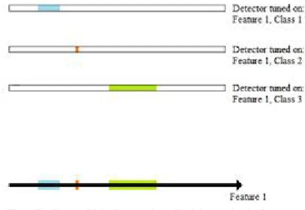
Example 2. In this example, an object is described by a set of N features (Fig. 18). The number of N = 3 will be used, for the sake of convenience. A set of a N sequence detectors will be necessary in this case, to identify any single class.In the
Figure 18. Case of three features, with three classes for everyone: a) Class 1 recognizer set.
b) Class 2 recognizer set. c) Class 3 recognizer set.
d) Single class domains, in the three dimensional feature space
© 2013 ACEEE
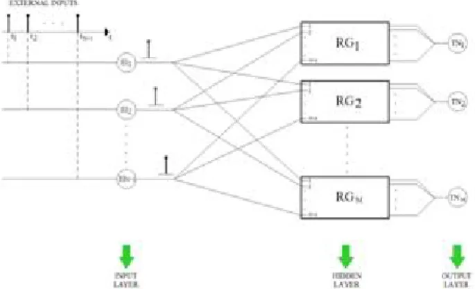
Fig. 19. The global architecture of the proposed SNN classifier.
A possible limitation of the previous procedure seems to be the shape of the class domains, which is always right-angled. In particular, a rectangle for a double feature, a paral-lelepiped for three feature, a hyper-paralparal-lelepiped in the gen-eral case. This limitation can easily be overcome using proper subclass groups implemented by different neural recognizers, linked to the same target. Structured Type RG could be ap-plied in this cases.A case of interest in the classification prob-lem is to grow up or down the action domains related to the identified classes (Fig. 20).
Fig. 20. Increase/Decrease of an action domain volume
As shown before, two external parameters can be used, in particular Pr and ld quantities. This possibility is very useful when different object could lie in adjacent zones in the feature space. In the case of multiple target activation, the proper change of the external parameters could get to the single target activation case. In similar way, if no target neurons are activated in correspondence to an input pattern, the corresponding class domain can be grow up, so that the interest point is included.
C. An Example: the “Art Paintings Classifier”
On the basis of the described structures, it could be possible
employ proper sequence detector sets for information recalling applications. The following example is an “art painting classifier” implemented. After a proper training, this “macro-structure” is able to recognize the art paintings. The training consists in the adjustment of the postsynaptic weights, with the aim of tuning the structures to the feature parameters; to do that statistical information are extracted from a reduced art painting data set to do that. For this purpose, the following five features (N=5) are considered: - Red Colour Dynamics
- Green Colour Dynamics - Blue Colour Dynamics - Edge Factor
- Size Factor
The feature selection is made so that the features were robust to rotations and resizing of the image in exam. For the feature extraction a MATLAB code is used.
Fig. 21. The detector group.
In Fig 21 the detector group relative to a single art painting is represented, in which each extracted feature is recognized by the related sequence detector. In this example, delayed spike timing sequence detector structures are used (see Fig 14). In this example are used the delayed spike timing sequence detectors. The detection of the features is possible only and if only the sequence detectors are tuned to the considered art painting. Then, an input features vector is provided to the detector group; this features are extracted by the test set. Moreover, is present an external target that fires only if at least 3 features are detected, then the art painting is correctly classified. Note that the external neuron is a simple combiner with a threshold, but without subthreshold decay. particular example shown , also the number of classes is 3.
B. Neural Architectures For Spike Timing Based Classifiers The design of the called timing based classifier consists of the following neural layers (Fig. 19).
An input neural layer able to receive the spike timing coded information. The external input number EI is equal to N + 1, in which N is the feature number related to each class. A hidden neural layer able to carry out the actual recognition of the interspike intervals. It consists of M recognizer group, where M is the class number.
An output neural layer consisting of the M target neurons. Each of these neurons will become active in correspondence to the related recognizer group (RG).
Fig. 22. The classifier.
The complete classifier structure (Fig. 22) consists of M-detector groups, where M is the number of considered art 87
© 2013 ACEEE
painting (that corresponds to the classes that the classifier have to recognize). The input features vector, of each considered art painting, is provided to all groups. The classification of a particular art painting occurs when the external target of the related group fires. As discussed above, the latter are sensitive to the specific art painting.
Below are shown the results obtained considering the following three art painting (M=3): Leonardo da Vinci’s “The Mona Lisa”, Edvard Munch’s “The Scream”, Vincent van Gogh’s “The Starry Night”.
The data set is consisted of 20 images, for each art painting, took from the internet. After the training, a test set, consisting of 8 images, for each art painting, not presented in the training, is presented to each tuned detector group. In the following table are illustrated the results, in terms of accuracy and precision of the classifier:
TABLE V. RESULTS OBTAINEDFROMTHE CLASSIFICATION
of sequence detectors could be used to solve complex classification problems, as the above example illustrated. In addition, the structures could be used to realize more complex systems to obtain analogic neural memories. In particular, proper neural chains could be useful as information memories, while proper sets of sequence detectors could be used for the information recalling.
REFERENCES
[1] W. Maass, “Networks of spiking neurons: The third generation of neural network models,” Neural Networks, vol. 10, no. 9, pp. 1659–1671, Dec. 1997.
[2] E. M. Izhikevich, “Which Model to Use for Cortical Spiking Neurons?,” IEEE Transactions on Neural Networks, vol. 15, no. 5, pp.1063–1070, Sep. 2004.
[3] E. M. Izhikevich, J. A. Gally, and G. M. Edelman, “Spike-timing dynamics of neuronal groups,” Cerebral Cortex, vol. 14, no. 8, pp. 933–944, Aug. 2004.
[4] A. Belatreche, L. P. Maguire, M. McGinnity, “Advances in design and application of spiking neural networks,” Soft Computing - A Fusion of Foundations, Methodologies and Applications, Vol. 11, pp. 239–248, 2007.
[5] G. L. Gerstein, B. Mandelbrot, “Random Walk Models for the Spike Activity of a single neuron,” Biophysical Journal, vol. 4, pp. 41–68, Jan. 1964.
[6] A. Burkitt, “A review of the integrate-and-fire neuron model: I. Homogeneous synaptic input,” Biological Cybernetics, vol. 95, no. 1, pp. 1–19, July 2006.
[7] A. Burkitt, “A review of the integrate-and-fire neuron model: II. Inhomogeneous synaptic input and network properties,” Biological Cybernetics, vol. 95, no. 2, pp. 97–112, Aug. 2006. [8] E. M. Izhikevich, “Polychronization: Computation with spikes,” Neural Computation, vol. 18, no. 2, pp. 245–282, 2006.
[9] S. Boudkkazi, E. Carlier, N. Ankri, et al., “Release-Dependent Variations in Synaptic Latency: A Putative Code for Short-and Long-Term Synaptic Dynamics,” Neuron, vol. 56, pp. 1048–1060, Dec. 2007.
[10] E. M. Izhikevich, Dynamical system in neuroscience: the geometry of excitability and bursting. Cambridge, MA: MIT Press, 2007.
[11] R. Brette, M. Rudolph, T. Carnevale, et al., “Simulation of networks of spiking neurons: A review of tools and strategies,” Journal of Computational Neuroscience, vol. 23, no. 3, pp. 349–398, Dec. 2007.
[12] M. D’Haene, B. Schrauwen, J. V. Campenhout and D. Stroobandt, “Accelerating Event-Driven Simulation of Spiking Neurons with Multiple Synaptic Time Constants,” Neural Computation, vol. 21, no. 4, pp. 1068–1099, April 2009. [13] M. Salern o, G. Su si, A. C ristini, “ Accu rate Latency
Characterization for Very Large Asynchronous Spiking Neural Networks,” in P roceedings of th e fourth Internation al C on ference on Bioin formatics Models, Meth ods an d Algorithms, 2011, pp. 116–124.
[14] A. L. Hodgkin, A. F. Huxley, “A quantitative description of membrane current and application to conduction and excitation in nerve,” Journal of Physiology, vol. 117, pp. 500–544, 1952. [15] J. H. Goldwyn, N. S. Imennov, M. Famulare, and Eric Shea-Brown. (2011, April). Stochastic differential equation models for ion channel noise in Hodgkin-Huxley neurons. Physical Review E. [online]. 83(4), 041908.
[16] R. FitzHugh, “Mathematical models of threshold phenomena
With the aim to determinate accuracy and precision, the following classical expressions are considered:
Accuracy = (TP+TN)/(TP+FP+FN+TN) Precision = TP/(TP+FP)
Where: TP is the number of true positives; TN is the number of true negatives; FP is the number of the false positives; FN is the number of the false negatives.
Note the good performance obtained by this simple classifier. Due to its low computational cost and the promising performance, this discussed structure could be useful for many other pattern recognition problems.
CONCLUSIONS
In this work a very simple and effective analog SNN model is presented, considering a basic biological neuron parameter: the spike latency. The firing activity, generated in the proposed network, appears fully asynchronous and the firing events consist of continuous time sequences. The simulation of the proposed network has been implemented by an event-driven method. The model has been applied to elementary structures to realize neural systems that generate or detect spike sequences in a continuous time domain.These neural structures, connected to a more high level, can realize a more complex structure able to process the information, operating a distributed and parallel input data processing. In this regard, the implementation of a SNN classifier is shown. An effective transformation of the input data domain into related spike timings domain is necessary, thus the temporal sequences obtained are processed by the classifier.In future works, sets
© 2013 ACEEE
in the nerve membrane,” Bull. Math. Biophys., vol. 17, pp. 257–278, 1955.
[17] NEURON simulator, available on: http://www.neuron.yale.edu/ neuron/
[18] L. F. Abbott, S. B. Nelson, “Synaptic plasticity: taming the beast,” Nature Neuroscience, vol. 3, pp. 1178–1183, 2000. [19] H. Z. Shouval, S. S. H. Wang, and G. M. Wittenberg, “Spike
timin g depen dent plasticity: a con sequ en ce of more
fundamental learning rules,” Frontiers in Computational Neuroscience, vol. 4, July 2010.
[20] T. P. Carvalho, D. V. Buonomano, “A novel learning rule for lon g-term plasticity of short-term syn aptic plasticity enhances temporal processing,” Frontiers in Computational Neuroscience, vol. 5, May 2011.
[21] G. M. Edelman, Neural Darwinism: The Theory of Neuronal Group Selection. New York, NY: Basic Book, Inc., 1987.