Investigation of synthetic strategies for enhancing the energy product of spinel ferrite nanoparticles

UNIVERSITA’ DEGLI STUDI DI SIENA

DIPARTIMENTO DI

BIOTECNOLOGIE, CHIMICA E

FARMACIA

DOTTORATO DI RICERCA IN SCIENZE

CHIMICHE E FARMACEUTICHE

XXXIII CICLO

COORDINATORE

Prof. Maurizio Taddei

Investigation of synthetic strategies for

enhancing the energy product of spinel ferrite

nanoparticles

SETTORE SCIENTIFICO-DISCIPLINARE CHIM/03

Dottoranda

Dott.ssa Beatrice Muzzi

_____________________________

Tutors

Dott. Claudio Sangregorio

_____________________________

Prof.ssa Fabrizia Fabrizi de

Biani

_____________________________

Contents

Chapter

1

Chapter

2

2.2 Magnetism in nanoscaled materials………...………....22

2.3 Interaction effects in nanostructures………..….………...26

2.4 Exchange-spring magnets…………...………...29

2.5 Exchange bias…………...……….34

2.6 Synthesis of magnetic nanoparticles……...………...40

2.7 The thermal decomposition technique……...…………...41

Chapter

3

3.2 Synthesis and characterization of NHS-2 and NHS-3……...………66

3.3 The key role of NaOL in the synthetic procedure……….76

3.4 Investigation of the reaction mechanism………..……….…80

Chapter

4

Tuning the Néel temperature of core|shell wüstite|magnetite

nanoparticles by doping with divalent metal ions_______________94 4.1 Morphological, structural and chemical composition analysis……..97 4.2 Magnetic properties of exchanged coupled CS nanoparticles…….113 4.3 Conclusions……….……….123

Chapter

5

Synthesis of FiM single phase NPs by mild oxidation process of AFM|FiM core|shell ______________________________________129 5.1 Morphological, structural and chemical composition analysis…....131 5.2 Magnetic characterization ……….…..149 5.3 Conclusions……….…….157

Chapter

6

Solvent mediated thermal annealing: a tool to enhance the coercivity of cobalt ferrite nanoparticles ______________________________160 6.1 Synthesis and characterization of CoyFe3-yO4 before and after solvent

mediated thermal annealing………....……….…………..162 6.2 Conclusions……….……….182

Chapter

7

Appendix_______________________________________________192

A.1 Instrumentation………....……….………..192

A.3.1 Starting materials and chemicals....……….194

A.3.2 Synthesis of Iron-Cobalt Oleate (x-FeCo(OL)) precursor…...…194

A.3.3 Synthesis of Co/CoyFe3-yO4 NPs: NHS-1, NHS-2 and NHS-3…195 A.3.4 The fundamental role of NaOL as reducing agent………...195

A.4.1 Starting materials and chemicals……….196

A.4.2 Oleate Precursors synthesis……….……….196

A.4.3 Synthesis of Fe1-xO|Fe3O4 (FeO) core|shell NPs……….196

A.4.4 Synthesis of CoxFe1-xO|CoyFe3-yO4 (CoFeO) and NizCoxFe 1-x-zO|NiwCoyFe3-w-yO4 (NiCoFeO) core|shell NPs…..………..……197

A.5.1 Synthesis of Fe3O4, CoFe2O4 and Ni0.4Co0.6Fe2O4 NPs...………197

A.6 Starting materials for Co0.4Fe2.6O4 NPs………..198

A.6.1 Synthesis of Co0.4Fe2.6O4 NPs……….….198

A.6.2 Solvent mediate thermal annealing of Co0.4Fe2.6O4 NPs….……199

Chapter

1

Introduction

In the last decades, the demand for new generation technology materials has pushed the research activity towards the development of nanomaterials. The nanosized materials reveal indeed excellent and unique optical, electrical, catalytic, medical, biological and magnetic properties, which arise from the finely tuned nanostructure (e.g. size, shape or by combining different nano-sized materials). In fact, below 100 nm several physical and chemical properties of the matter are strongly altered with respect to the bulk counterparts and novel phenomena are observed (see section 2.2 Magnetism in nanoscaled materials). In the last years, the increased capability of shaping matter at the nanoscale to create complex hybrid architectures has represented a major step forwards in the nanoscience to develop innovative and multifunctional materials. Combining components at the nanoscale endowed with different physical properties, either strongly interacting or not, can indeed largely expand and enhance the material functionalities, and, in some cases, enable the emergence of new properties. The resulting multifunctional nanomaterials are then promising candidates to address many of the challenges of the next future in a wealth of research areas, ranging from biomedicine to electronics (Table 1.1). In this regard, magnetic hybrid nanostructures are particularly promising.

Table 1.1 Schematic classification of main applications for nanomaterials.

Area of interest Application Examples

Biological Diagnosis ((fluorescence labelling, contrast agents

for magnetic resonance)1,2,3

Medical therapy (drug delivery, hyperthermia)4,5,6

Chemical Catalysis (fuel cells, photocatalytic devices and

production of chemicals)7,8,9

Electronic High performance delicate electronics10

High performance digital displays11,12

Energetic High performance batteries (longer-lasting and

higher energy density)13 High-efficiency fuel cells14

High-efficiency solar cells15

Magnetic High density storage media16

Magnetic separation17

Highly sensitive biosensing18 Permanent magnets19

Mechanical Mechanical devices with improved wear and tear

resistance, lightness and strength, anti-corrosion abilities10,20

Optical Anti-reflection coatings21

Specific refractive index for surfaces22 Light based sensors23

Coupling at the nanoscale materials with intrinsically different magnetic properties, indeed, allows the observation of novel magnetic phenomena, the most prominent being exchange bias and exchange spring coupling. The former originates from the exchange interactions between differently ordered magnetic phases, usually an antiferromagnet (AFM) and a ferro- or ferrimagnetic (F(i)M) one,24 while the second is obtained by combining at the nanoscale a high anisotropy hard magnetic phase with a high magnetization soft magnetic phase (for further information see section 2.4 and 2.5 in Chapter 2).25

These phenomena have been proposed in the recent past as efficient strategies to enhance the performances of permanent magnets (PM).26–28

PM are key elements in modern technology as they allow storing, delivering and converting energy. In particular, in generators, actuators and motors, they are able to transform electrical energy into mechanical and vice versa. The possibility of maintaining large magnetic flux both in the absence of an applied magnetizing field and upon modification of the environment (demagnetizing field, temperature, etc.) is a unique feature which allows permanent magnet to be used in a wide variety of applications (figure 1.1)

Figure 1.1 Image of magnetic nanoparticles (NPs) and a list of applications for

permanent magnets.

Magnets, are in fact used as constituents in low-carbon renewable energy application (wing turbines, wave parks generators, flywheels), future mobility technologies (electric vehicles) and of a broad range of high-tech products. Being ubiquitous components, PMs represent a worldwide market that is expected to amount to 33.65 billion € by 2025, which is the consequence of an 8.3% annual increase (CAGR) predicted for the next five years.29 The efficiency of a material to act as a permanent magnet relates to its ability of store magnetostatic energy, which is commonly quantified by the maximum energy product (BHmax). Figure 1.2 highlights

Figure 1.2 a) Typical magnetization (M) and b) magnetic induction (B)

dependence on the applied field (H) for a permanent magnet. The load line (dashed), working point, and the maximum energy product (BHmax, given by the

area of the shaded rectangle) all depend on the magnet shape. Modified by Ref (30_).

When a permanent magnet is placed in a magnetizing field (H) the magnetization/induction (M/B) increase with H until the material is fully magnetized (saturation point, MS). When H is gradually reduced to zero,

the magnetization of the material decreases from MS down to a value, MR,

known as remanence, (or residual magnetic density flux, BR). If H is then

increased in the negative direction, MR is reduced to zero at the so-called

coercive field, -HC. The area of the largest rectangle that can be inscribed

under the demagnetizing branch at negative fields (the second quadrant) in the B(H) loop, corresponds to the maximum energy product (BHmax).

The working point corresponds to the B,H values in the operating conditions of a permanent magnet and depends on the external field and on the B(H) curve (internal field, magnet shape, etc.).30,31

Large BHmax values are found in magnets characterized by high saturation

magnetization and large remanence values (which is proportional to the magnetic field they create in the absence of any external magnetizing

field). Moreover, to avoid demagnetization due to internal and external fields, it is important to have a large coercivity and thus large magnetic anisotropy and high Curie temperature, TC, are required. In nature, it is

hard to come across a material that unites these requisites, so that often one of them is gained at the expense of the others. Indeed, materials characterized by large saturation magnetization, such as the transition metals (TM) Fe, Co and Ni and their alloys, normally show low magnetic anisotropy. The largest magnetic performance is obtained for materials composed of rare earths (RE) and TM, like Nd2Fe14B and SmCo5, that

have huge magnetic anisotropy, high average magnetization and large TC.

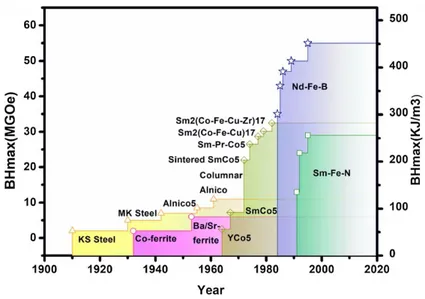
The energy product of RE-based permanent magnets is between 200 and 450 kJm-3. Permanent magnets made of ferrites and alnicos, the other two main families of magnetic materials, barely grasp 50-100 kJm-3 (figure 1.3)32,33.

Figure 1.3 Plots of BHmax values of different permanent magnets developed over

the years32_.

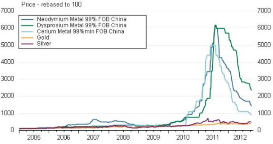
From these considerations, RE-based magnets are required for high performance applications or micro-scalable devices of high technological impact due to their performance-to-size ratio. However, with China accounting for 77% of the world RE production in 2019, the production of devices containing RE elements is potentially subject to price fluctuations which may arise from restrictive export politics. Actually, the possibility of sudden price oscillations come into reality in 2011 during the so-called “RE-crisis” when, as reported in Figure 1.4, the cost increase of RE exceeded 600% in few months, after some restrictions imposed to the exportation in RE-based raw-materials towards Japan.

Figure 1.4 Rare earths vs. gold and silver price increases from 2005 to 2012:

2011 “RE-crisis” is delineated by peaks in Nd, Dy and Ce price rise.31

The criticality of RE, associated not only to their supply risk and price volatility, but to their harmful environmental impact as well, has brought forward the realization that it is of great sustainable, strategic, geographic and socio-economic importance to reduce their use in high-tech sectors which drive the permanent magnet market. The trade disputes between China and the United States can lead to supply disruptions, in a landscape where already in 2018, the mining of RE did not cover the worldwide demand and material had to be supplied from stockpiles. Demand and supply problems have been forecast from 2021 onwards. The problem will be worsened by the projected increased use of RE in wind power generators and electric cars in the next 10 years. The situation pressingly demands innovations that lead to a substitution of RE by non-critical materials in these devices, as the impact of a supply disruption on the associated European industries may reach billions of euros and affect jobs.29

It is important to stress that a number of key technologies rely on magnets with moderate energy products within the range 50-200 kJm-3_{. This “no}

man's land” application area includes fundamental fields such as diverse components for transport (mainly automotive industry) and energy (with new generation of friendly environmental platforms such as wind turbines or photovoltaics, and more classical ones such as refrigeration motors). Nowadays this gap is filled by low performing RE magnets, but it is important to consider alternative magnets RE-free. It is crucial to keep in mind that the ultimate success of these alternatives, in terms of socioeconomic impact, is of course intimately related to the cost-efficiency and the sustainability of the associated fabrication processes. It has been shown for “already effective” RE-based permanent magnets that their performance can be significantly improved through their microstructure and the composition optimization34,35. Therefore, it can be argued that the same approach would result in similar improvements on the magnetic properties of transition metal-based nanostructures. The research on nanostructured ferrites and transitions metal alloys thus has grown exponentially, with the purpose to understand the correlation between properties and material nanostructure and achieving enhanced performances for permanent magnet applications19,36,33,27,26,37,38,39,40_.

The aim of this work is the synthesis and study of new materials to develop permanent magnets which do not completely replace those including rare earths, but, despite of a lower BHmax value than that of NdFeB, have

however higher performances than commercial ferrites currently available in the market (i.e. strontium ferrites). Even if some transition metals, like cobalt, are critical elements, it is important to underline that since this is

an exploratory work, we chose materials and synthetic methods that privileges the fine control on the chemical and physical properties of the final product, at the expenses of large scale production. The present work is in fact focused on the study of quasi-zero-dimensional magnetic material and the different possible strategies (i.e. exchange coupling between two materials and solvent mediated thermal annealing) for improving the performance of spinel ferrites. In particular, novel nanosized hybrid permanent magnets based on the interaction of magnetic materials with complementary properties to achieve outstanding magnetic performances, are investigated. As a first step, the hybrid nanocomposite magnets are designed on the basis of an effective exchange-coupling through the interface of hard and soft magnetic constituents (exchange spring effect) or AFM and F(i)M phases (exchange bias effect). The exchange coupling effects, despite still under investigation, have been already proposed as a viable strategy for increasing the performance of permanent magnets. In fact, the coupling of hard magnetic phase with a soft one leads to an increase of the saturation magnetization (MS), of the remanence (MR) and

to a moderate decrease of the coercive field of the hard phase (exchange spring effect). Instead, the coupling of AFM and F(i)M phases is followed by an increase of the coercive field of the final coupled system (exchange bias effect). The effectiveness of the exchange-coupling depends on the intergrain exchange interaction between neighbouring grains which causes the spontaneous magnetization of each individual grain to deviate from its particular easy axis towards the direction of the polarization of the nearest ones. This phenomenon can be important for permanent magnet: a theoretical model has predicted an increase of BHmax for materials

In the second step, we investigated the possibility of improving the magnetic performances of the prepared nanomaterials by post-synthesis processing. To this aim we explored two different synthetic approaches which were applied to core|shell AFM|F(i)M hybrid NPs and standard ferrites, respectively. The first one relies on the mild oxidation of the core|shell NPs realized by solvent mediated annealing in the presence of air. It is expected that the mild oxidation of the NPs would transform the antiferromagnetic core in ferrimagnetic ordered ferrite, allowing at the same time the formation of a mosaic texture of small subdomains, separated by antiphase boundaries. These, in turn, can be still responsible of the occurrence of exchange bias phenomena, leading to the increase of the coercive field in the new formed ferrite. The second proposed approach is the solvent mediated annealing treatment of standard ferrites. As it is well known, the reduction at the nanoscale of the classical ferrites is followed by the increase of the intrinsic anisotropy value42. At the same time, the nanosized material is also affected by a high crystallographic microstrain value. The solvent mediated annealing treatment is proposed as a good approach to reduce the internal stress generated during the crystallographic growth, leading to the enhancement of the coercive field value and thus of the magnetic performance of the material.

This thesis is structured in the following sections:

Chapter 2 reports a brief summary of the theory of magnetism and the behaviour of magnetic material, with a particular attention to hybrid nanostructured systems and the related interaction effects, such as exchange bias and exchange spring magnet. A short discussion of the theoretical principles of the preparation technique of 0D materials adopted in this work is also provided.

Chapter 3. In this chapter is reported the synthesis and characterization of cobalt/cobalt ferrite (Co(0)/CoyFe3-yO4) nano-heterostructures (NHSs) with

high crystallinity and controlled composition. Moreover, it describes the study of the reaction mechanism and of the role of each parameters in the synthetic procedure, i.e the precursor/stabilizing agent molar ratio, the nature of the metal precursor and the decomposition time. This investigation allows us to optimize the synthetic method and obtain nano-heterostructures with the desired magnetic properties.

Chapter 4 Here is reported the study of iron based exchange coupled core|shell AFM|F(i)M NPs doped with different divalent ions (Co(II) _and

Ni(II)_{) synthetized by thermal decomposition of bi- or trimetallic oleate}

precursor. After the morphological and chemical investigation of the samples, a detailed magnetic characterization is performed with the aim to understand how the substitution of Fe(II) with Co(II) and Ni(II) can modify the magnetic properties and how the different ions distribution changes the exchange bias effect.

Chapter 5 In this chapter is reported the synthesis and crystallographic characterization of cubic spinel ferrites doped with divalent ions (cobalt and nickel) obtained after mild oxidation - solvent mediated process of

core|shell AFM|F(i)M NPs. In particular, the internal crystal lattice deformation and the resulting magnetic properties of the obtained magnetite are investigated as a function of the doping with the Co(II) and Ni(II).

Chapter 6 The chemical-physical characterization of narrowly distributed cobalt ferrite NPs before and after solvent mediated thermal annealing, is reported. In particular, the crystal lattice deformation with the corresponding magnetic properties are investigated as a function of the annealing temperature and the NPs’ environment where the heating processes is carried out.

Chapter 7 The final section briefly summarizes the main conclusion gained from the experimental work presented above and the future perspectives of these materials as building blocks for the realization of RE free permanent magnets.

Appendix The main experimental techniques and the operative procedure used during this work are reported and discussed.

References

1 V. A. Sinani, D. S. Koktysh, B. G. Yun, R. L. Matts, T. C. Pappas, M. Motamedi, S. N. Thomas and N. A. Kotov, Nano Lett., 2003, 3, 1177–1182.

2 Y. Zhang, N. Kohler and M. Zhang, Biomaterials, 2002, 23, 1553–1561.

3 T. J. Yoon, H. Lee, H. Shao and R. Weissleder, Angew. Chemie -

Int. Ed., 2011, 50, 4663–4666.

4 J. Gao, H. Gu, B. Xu, Prog. Chem., 2009, 42, 1097–1107.

5 A. Solanki, J. D. Kim and K. B. Lee, Nanomedicine, 2008, 3, 567– 578.

6 O. Salata, J. Nanobiotechnology, 2004, 2, 1–6.

7 H. L. Xin, J. A. Mundy, Z. Liu, R. Cabezas, R. Hovden, L. F. Kourkoutis, J. Zhang, N. P. Subramanian, R. Makharia, F. T. Wagner and D. A. Muller, Nano Lett., 2012, 12, 490–497.

8 Z. Liu, Y. Qi and C. Lu, J. Mater. Sci. Mater. Electron., 2010, 21, 380–384.

9 A. Murugadoss, P. Goswami, A. Paul and A. Chattopadhyay, J.

Mol. Catal. A Chem., 2009, 304, 153–158.

10 F. R. Marciano, L. F. Bonetti, R. S. Pessoa, J. S. Marcuzzo, M. Massi, L. V. Santos and V. J. Trava-Airoldi, Diam. Relat. Mater., 2008, 17, 1674–1679.

12 J. E. Millstone, D. F. J. Kavulak, C. H. Woo, T. W. Holcombe, E. J. Westling, A. L. Briseno, M. F. Toney and J. M. J. Fréchet,

Langmuir, 2010, 26, 13056–13061.

13 C. D. Wessells, R. A. Huggins and Y. Cui, Nat. Commun., 2011, 2, 550–555.

14 B. Bogdanović, M. Felderhoff, S. Kaskel, A. Pommerin, K. Schlichte and F. Schüth, Adv. Mater., 2003, 15, 1012–1015. 15 X. Chen, B. Jia, J. K. Saha, B. Cai, N. Stokes, Q. Qiao, Y. Wang,

Z. Shi and M. Gu, Nano Lett., 2012, 12, 2187–2192. 16 G. Reiss and A. Hütten, Nat. Mater., 2005, 4, 725–726.

17 I. S. Lee, N. Lee, J. Park, B. H. Kim, Y. Yi, T. Kim, T. K. Kim, I. H. Lee, S. R. Paik and T. Hyeon, 2006, 128, 10658–10659. 18 H. Lee, T. J. Yoon and R. Weissleder, Angew. Chemie - Int. Ed.,

2009, 48, 5657–5660.

19 G. C. Papaefthymiou, Nano Today, 2009, 4, 438–447.

20 L. Shi, D. S. Shang, Y. S. Chen, J. Wang, J. R. Sun and B. G. Shen, J. Phys. D. Appl. Phys., 2011, 44, 455305.

21 K. C. Krogman, T. Druffel and M. K. Sunkara, Nanotechnology, 2005, 16, 338–343.

22 H. Chen, X. Kou, Z. Yang, W. Ni and J. Wang, Langmuir, 2008, 24, 5233–5237.

23 J. N. Anker, W. P. Hall, O. Lyandres, N. C. Shah, J. Zhao and R. P. Van Duyne, Nat. Mater., 2008, 7, 442–453.

24 W. H. Meiklejohn and C. P. Bean, Phys. Rev., 1956, 102, 1413– 1414.

25 H. Zeng, J. Li, J. P. Liu, Z. L. Wang and S. Sun, Nature, 2002, 420, 395–398.

26 E. F. Kneller and R. Hawig, IEEE Trans. Magn., 1991, 27, 3588– 3560.

27 F. Jimenez-Villacorta and L. H. Lewis, in Nanomagnetism, ed. J. M. Gonzalez Estevez, One Central Press, 2014, 160–189.

28 J. Sort, J. Nogués, S. Suriñach, J. S. Muñoz, M. D. Baró, E. Chappel, F. Dupont and G. Chouteau, Appl. Phys. Lett., 2001, 79, 1142–1144.

29 G. V. Research, 2020.

30 J. M. D. Coey, Engineering, 2020, 6, 119–131. 31 E. Lottini, PhD Thesis, 2016, 145.

32 A. Sarkar and A. Basu Mallick, Jom, 2020, 72, 2812–2825. 33 O. Gutfleisch, M. A. Willard, E. Brück, C. H. Chen, S. G. Sankar

and J. P. Liu, Adv. Mater., 2011, 23, 821–842.

34 S. Sugimoto, J. Phys. D. Appl. Phys., 2011, 44, 064001 (11pp) 35 J. M. D. C. Skomski, Ralph, Phys. Rev. B., 1993, 48, 15812–

15816.

36 A. H. Lu, E. L. Salabas and F. Schüth, Angew. Chemie - Int. Ed., 2007, 46, 1222–1244.

38 A. López-Ortega, M. Estrader, G. Salazar-Alvarez, A. G. Roca and J. Nogués, Phys. Rep., 2015, 553, 1–32.

39 J. Nogués, J. Sort, V. Langlais, V. Skumryev, S. Suriñach, J. S. Muñoz and M. D. Baró, Phys. Rep., 2005, 422, 65–117.

40 M. Vasilakaki, K. N. Trohidou and J. Nogués, Sci. Rep., 2015, 5, 9609.

41 E. F. Kneller and R. Hawig, IEEE Trans. Magn., 1991, 27, 3588– 3600.

42 A. López-Ortega, E. Lottini, C. D. J. Fernández and C. Sangregorio, Chem. Mater., 2015, 27, 4048–4056.

Chapter

2

Magnetism in nanoparticles

This thesis is focused on the synthesis and investigation of the magnetic behaviour of novel nanostructured materials. Thus, in this Chapter the basic concepts of the physical behaviour of magnetic materials and, particularly, of magnetic nanoparticles, are briefly reviewed.

2.1 Magnetic materials

Any substance in the presence of an external applied magnetic field (H) gives rise to a response, known as magnetic induction (B). The relationship between B and H depends on the material (Equation 2.1):

𝑩 = 𝜇0(𝑯 + 𝑴) (2.1)

In equation 2.1 μ0 is the vacuum permeability (μ0 = 4π·10-7 Hm-1) and M

the magnetization of the material. The magnetization depends on the applied field and, when H is not too large, is proportional to H, the proportionality constant, χ, being known as magnetic susceptibility. The magnetic susceptibility is a property of the material and it is commonly used to classify different magnetic behaviours. More in detail, the magnetic moment of a material and, thus, its magnetic susceptibility, depends on the electron configuration of the individual atoms.

I) Diamagnetic (χ < 0). In the presence of an applied field, all atoms display the diamagnetic effect, i.e., a change in the orbital motion of the electrons producing a field opposing to the external one. In fact, when the magnetic field is applied, extra currents are generated in the atoms by electromagnetic induction. In accordance with the Lenz law, the current generates an induced magnetic moment proportional to the applied field and with opposite direction.Diamagnetism is such a weak phenomenon that only those atoms that have no net magnetic moment, i.e., atoms with completely filled electronic shells, are classified as diamagnetic.

II) Paramagnetic (χ > 0). Paramagnetic (PM) materials have unpaired electrons and, thus, present a net atomic magnetic moment. However, atomic magnetic moments have only weak exchange interaction with their neighbours and the thermal energy causes their random alignment. In the presence of an applied field, the atomic moments start to align resulting in a macroscopic magnetization of the material, while when the field is turned off the material has no net magnetic moment. III) Ordered magnetic materials. Ferromagnetic (FM),

ferrimagnetic (FiM) and antiferromagnetic (AFM) materials have unpaired electrons such as paramagnetic one. However, these materials present a strong exchange interaction between atomic moments compared to thermal energy, thus, they are characterized by an ordered network of magnetic moments at room temperature. The magnetic moment can be aligned in parallel or antiparallel (Figure 2.1).

Figure 2.1 Schematic description of magnetic moment order in magnetic

materials1_.

FM materials have all atomic magnetic moments parallel one to each other and are characterized by the presence of a net magnetic moment even without an applied field. This spontaneous magnetization is maximum at 0 K, (M0), where all the atomic moments are perfectly aligned in parallel.

As the temperature increases, the thermal energy introduces some disorder in the alignment, which makes the magnetization to decrease, until a critical temperature, called Curie temperature (TC), is reached, where the

thermal energy overcomes the exchange interaction and the material assumes a PM behaviour.

Below TC, FM materials are characterized by magnetic irreversibility,

which is associated with the energy required for the magnetization reversal. Thus, when the magnetic moments are oriented by an external positive magnetic field, in order to attain a demagnetized state it is necessary to apply a negative magnetic field (coercive field) or to increase the temperature above TC.2 FM materials can be divided in two categories

“hard” and “soft”, on the base of the strength of the applied magnetic field required to align the magnetic moment. Soft magnets have high magnetic permeability, with low coercive field (HC) and high saturation

magnetization (MS), while hard materials have low magnetic permeability

and moderate MS, but high HC and magnetic remanence (MR).

Figure 2.2 Hysteresis curve of hard (red line) and soft (blue line) magnetic

materials.

FiM and AFM materials present an antiparallel alignment of neighbouring atomic magnetic moments. Such materials can be schematized through the combination of two antiparallel coupled magnetic sub-lattices, inside of which magnetic moments are parallel aligned. In AFM materials the magnetic sub-lattices compensate each other nullifying the total magnetization, while in FiM systems they have different values resulting in a net magnetization. Therefore, FiM materials can be imaged as FM ones where the net magnetization corresponds to the difference between the values of the two sub-lattices. Consequently, also FiM materials exhibits spontaneous magnetization till a characteristic ordering

temperature (TC) is reached, above which the material becomes PM and its

susceptibility follows the Curie-Weiss law (Equation 2.2):

χ = 𝐶

𝑇 − 𝜃 (2.2)

where  is the Weiss constant and is related to the strength of the magnetic moment interaction (for a FM =TC). Similarly, AFM materials are

characterized by an ordering temperature, called Néel temperature (TN), above which they behave like PM phases.

2.2 Magnetism in nanoscaled materials

Matter behaves differently when its size is reduced to the nanoscale. In general, below 100 nm, when the material size is comparable with the characteristic length scale of many physical phenomena (e.g. electron mean free path, domain wall width, diffusion length, superconducting coherent length, etc.), chemical and physical properties are affected by

finite-size effects. In particular, the domain wall thickness, which falls in

the nanometric range, is one of the characteristic lengths affecting material magnetic behaviour. Moreover, the large increase in the ratio between surface and volume, typical of the nanostructures, produces further surface

effects. The formation of magnetic domains in bulk materials occurs in

order to reduce the magnetostatic energy of the system. However, when the size of the material becomes smaller than the domain walls thickness, the energy gain obtained by the formation of a multi domain structure is lower than the energy spent for the wall formation, leading to a single domain system. The main consequence of being in the single domain state is that changes in the material magnetization can no longer occur through

domain wall motion, but require the rotation of all the spins, resulting in an enhancement in the coercivity of the system.

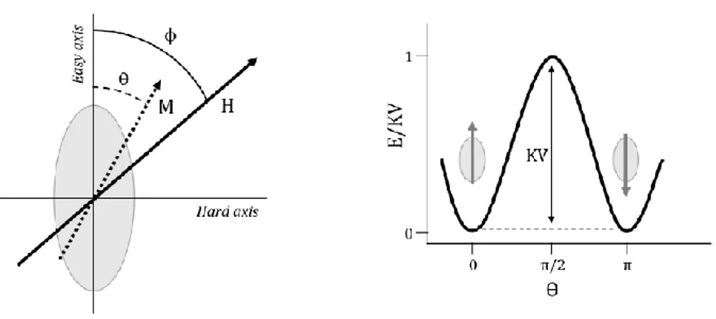
In single domain nanoparticles the Stoner and Wohlfarth model3 describes the energy related to the magnetization reversal in terms of the material anisotropy. The model assumes a coherent rotation of all the spin in a particle and the presence of a uniaxial anisotropy (the system is characterized by a single easy axis of magnetization). Thus, the energy density of the system can be written as:

𝐸_𝐵= 𝐾𝑉𝑠𝑖𝑛2(𝜃) + 𝐻𝑀_𝑆cos(𝜙 − 𝜃) (2.3) where ϴ is the angle between M and the magnetization easy axis, and ϕ the angle between H and the magnetization easy axis (see Figure 2.2). In particular, the first term (KVsin2(ϴ)) refers to the magnetic anisotropy and

the second one (HMScos(ϕ−ϴ)) is the Zeeman energy corresponding to the

torque energy on the particle moment exerted by the external field. As illustrated in Figure 2.3, when H=0 the Zeeman term is zero and there exist two equilibrium states for ϴ=0 and ϴ=π. The energy barrier separating these two states is equal to KV. This is the magnetic anisotropy energy of the system,4 and corresponds to the energy for the magnetization reversal to occur1.

Figure 2.3 Stoner and Wohlfarth model: definition of the axis system (left) and

angular dependence of the energy for a zero external field (right).1

In the presence of an applied field, for a fixed temperature, the Zeeman term can modify the particle energy. If H < 2K/MS the system energy

maintains two minima although they are no more equivalent in energy; instead, if H ≥ 2K/MS only a single minimum will be present. The H value

above which the energy of the system presents only one minimum (H0 =

2K/MS) is called anisotropy field.

As already reported above, the energy barrier of a single domain particle with uniaxial anisotropy is KV, and it becomes increasingly smaller with the decreasing of the volume. Eventually, for particle of few nanometers, the term KV becomes sufficiently small, that, even in the absence of an external field, the thermal energy (kBT, where kB is the Boltzman's

constant) is sufficient to induce magnetic fluctuations and spontaneous reverse of the magnetization from one easy direction to the other. In these conditions the system behaves like a paramagnet (see section 2.1), but with much higher value of magnetic moment, being the sum of 102-105 spins; this state is called superparamagnetic state.5,4,6 _{The temperature at which}

the system reaches the superparamagnetic state depends on particles volume and anisotropy.

We can introduce a relaxation time (τ) for the magnetization reversal process:

𝜏 = 𝜏0exp (

𝐾𝑉 𝑘𝐵𝑇

) (2.4)

where τ0 is a time constant characteristic of the material and usually is of

the order of 10-9-10-12 s for non-interacting ferro/ferrimagnetic particles. The magnetic behaviour of single domain particles is then strongly time dependent, i.e. the observed magnetic state of the system depends on the characteristic measuring time of the used experimental technique, τm.

Therefore, it can be defined a temperature, called blocking temperature (TB), at which the relaxation time equals the measuring one (τ = τm):

𝑇_𝐵 = 𝐾𝑉 𝑘_𝐵𝑙𝑛 (𝜏_𝜏𝑚

0)

(2.5)

Consequently, being TB dependent on the time scale of the measurements,

for experimental techniques with τm > τ the system reaches the

thermodynamic equilibrium in the experimental time window and a superparamagnetic behaviour is observed. Conversely, when τm < τ

quasi-static properties (similar to bulk materials) are obtained, i.e. the particles are in the blocked regime. Thus, a nanoparticles’ assembly at a given temperature can be either in the superparamagnetic or blocked regimes, depending on the measuring technique.

It is important to remind that the equations 2.4 and 2.5 are obtained for monodisperse and non-interacting single domain nanoparticles. In a

system with inter-particles interaction TB can be increased by the extra

energy terms introduced by the dipolar and/or exchange interaction. The reduction of the particles size to the nanoscale leads to further modification in the material magnetic behaviour due to the increased ratio between surface and volume. Indeed, in few nanometres particles, the number of atoms on the surface is no longer negligible with respect to the inner atoms and surface effects become relevant. The symmetry breaking occurring at the surface modifies the intrinsic single-ion properties of surface atoms leading to enhanced anisotropy and surface spin disorder,7,4 e.g. canted spin, frustration and spin-glass behaviour. In particular, spin

canting arises from the crystal lattice deformation due to the different

coordination of the surface atom which leads to a change in the exchange coupling magnetic constant (J) of the material.

2.3 Interaction effects in nanostructures

The magnetic field produced by blocked nanoparticles can interact with the magnetic moment of neighbouring nanoparticles by short-range exchange interaction and long-range anisotropic interaction, known as dipole-dipole interaction (Equation 2.6). In the limit of weak interactions, the dipole energy (Ed) depends on the number of nearest neighbours, the n1, and on ε and z which are proportional to the magnetic moment and the

geometrical arrangement:

𝐸_𝑑 = 𝑛1ε

2_(3𝑧2 _{− 1)}2

The energy barrier KV of each particles is modified by the dipole-dipole interactions and in the limit of the weak interactions becomes:

𝐸_𝑎 = 𝑉(𝐾 + 𝐻_𝑖𝑛𝑡𝑀) (2.7)

where Hint represents the mean interaction field.8 Extensive experimental

and theoretical works agree that the interaction among magnetic particles plays a fundamental role in the magnetic behaviour of granular systems9,10,11,12,13,14_{. Despite of this, there exist several inconsistencies}

between the theoretical models that describe different behaviour of TB as

a function of the dipolar interactions. For example Shtrikman et al.8 predicted the increase of the TB with strength of the dipolar interactions,

i.e. increasing particle concentration or decreasing particle distance8,11,10, while, in the weak interaction limit, Dormann et al.10,11 proposed the opposite dependence of TB with the dipole-dipole interaction

strength10,11,12,14.

Dipole-dipole interactions in randomly oriented nanoparticles can also affect the shape of the hysteresis loop in magnetic nanoparticles, due a decreasing in the energy barrier of the system and thus to its coercivity15,16,17. Conversely, when the particles are not randomly oriented the coercivity can increase or decrease depending on the type of arrangement.18,19

If nanoparticles are in close proximity, exchange interactions between surface atoms can also be operative due to the overlap of their wave functions, resulting in a modification of the energy barrier of the whole system (Equation 2.8).20

𝐸 = 𝐾𝑉𝑠𝑖𝑛2_{𝜃 − 𝐽}

𝑀⃗⃗ (𝑇) represents the sub-lattice magnetization vector of a particle at temperature T, and Jeff is an effective exchange coupling constant so that

Jeff⟨𝑀⃗⃗ (𝑇)⟩ describes the effective interaction mean field acting on 𝑀⃗⃗ (𝑇).

The exchange and dipolar interactions between nanoparticles also change the relaxation process; indeed, equation 2.4 for the relaxation time is modified in:

𝜏 = 𝜏₀exp (𝐾𝑉 𝑘_𝐵𝑇+

𝐸_𝐵𝑖

𝑘_𝐵𝑇) (2.9)

where EBi is the interaction anisotropy expressed as: EBi = n1ε(3z2

-1)L[ε(3z2-1/kBT)] and it depends on n1, ε and z and L is the Langevin

function, L(x) = coth(x)-1/x. The equation 2.9 in the limit of the weak interactions can be thus written as:

𝜏 = 𝜏₀exp (𝐾𝑉 𝑘_𝐵𝑇+

𝑛1ε2(3𝑧2− 1)2

3𝑘_𝐵2𝑇2 ) (2.10)

For nanoparticles in close proximity (strong interaction case) the interactions contribute cannot be considered anymore as perturbation and the nanoparticles’ assembly must be considered as a collective system. For such a system the relaxation time is then expressed as21:

𝜏 = 𝜏0exp(−𝑛1)𝑒𝑥𝑝 ( 𝐾𝑉 𝑘𝐵𝑇 +𝑛1ε 2_(3𝑧2_{− 1)}2 𝑘𝐵𝑇 ) (2.11)

The same consideration can be done when two different materials are in direct contact, which if strong exchange interaction, can be considered as a single system. The exchange interactions between two magnetic materials can lead to interesting behaviour especially when materials with

different magnetic behaviour are coupled. In particular, the two more prominent exchange effects that can appear are:

(I) Exchange-spring arising from the coupling of interface contact between two FM, or FiM, phases with hard and soft properties.

(II) Exchange bias originated usually from the interface contact between an AFM phase and a FM, or FiM, one. However, it can occur in other type of bi-magnetic systems as FM-FM, FiM-FiM or spin-glass materials. These effects appear in hybrid nanostructure, e.g. thin films, core|shell nanoparticles or heterodimers, where the different magnetic phases are in direct contact.

2.4 Exchange-spring magnets

In the literature, studies on exchange-spring magnets are basically performed with the aim to enhance the permanent magnet performances, producing new magnets characterized by an increased area of the hysteresis loops. Kneller et al.22 _{first proposed as a new strategy to develop}

permanent magnets, the coupling through exchange interactions of a hard-FM phase, characterized by high magnetocrystalline anisotropy (large HC),

and a soft phase with high magnetic moment (large MS) are, producing the

so-called exchange-spring permanent magnet. The resultant material has display a hysteresis loop which maintains the high HC, close to that of the

hard phase and a large MS, close to that of the soft phase23.

The exchange coupling results indeed in the modification of the remanence (R = MR/MS), coercive field and demagnetizing curve, as schematized in

uniaxial magnetocrystalline anisotropy and isotropic distribution of easy axes, MR = 0.5MS.3 However, if neighbouring grains of hard and soft phase

are coupled through exchange interaction, at the interface the magnetic moments of the soft phase are aligned with those of the hard one, resulting in MR > 0.5MS. In addition, interfacial atoms of the soft phases are

characterized by a larger coercivity, which tends to that of the hard one, while the hard phase shows reduced coercivity. Indeed, when the demagnetizing field reverses the moments in some soft grains, they tend to reverse the moments in the neighbouring hard ones by exchange coupling. As a result, the final coercive field of the system assumes an intermediate value between those of the two magnetic phases. Moreover, also the demagnetization curve will be modified, its shape depending on the entity of the exchange coupling between the two phases. If the whole soft phase is exchange-coupled with the hard one, both phases reverse their magnetization at the same nucleation field (HN) and the demagnetizing

curve in the second quadrant is convex, like for a single-phase material. Conversely, if only a fraction of the entire soft phase is coupled, the magnetization reversal of the uncoupled fraction of soft phase occurs at significantly lower fields than the HN of the system. Hence, the

demagnetizing curve in the second quadrant has a concave shape. Another characteristic of exchange-spring magnets is that in the demagnetizing process, the reversal of magnetic moments is reversible when the applied field is smaller than HN, i.e. before the hard phase starts to reverse its

magnetization. In fact, for H < HN the moments of the soft phase can

already have reversed their magnetization and, as the field is removed, they return reversibly to their original direction due to the coupling with the hard phase. Thus, due to the large contribution of the soft phase to the final M value, the reversible magnetization of the hard-soft two-phase

magnets is much larger than that of conventional hard magnets. Therefore, the magnetic behaviour recalls that of a mechanical spring, whence the name spring-magnet.

Figure 2.4 Scheme of typical demagnetization curves M(H) in bi-magnetic

systems. Top: exchange-spring magnet with tS ≤ tS,c (left) and tS > tS,c (right)

Bottom: conventional single ferromagnetic phase magnet (left) and mixture of two independent ferromagnetic phases with largely different hardness (right).22

All these modifications in the magnetic behaviour are strictly affected by the fraction of exchange-coupled soft phase and by its thickness (tS). In

particular, there exists a critical thickness of the soft phase (tS,c), below

which the system is completely exchange-coupled, corresponding roughly to twice the width of a domain wall in the hard phase (δH):

𝑡_𝑆,𝑐 = 2𝛿𝐻 = 2 (𝜋√𝐴𝐻

𝐾_𝐻) (2.12)

where AH and KH are the exchange and anisotropy constants of the hard

phase, respectively. However, two cases are distinguished: when tS ≤ tS,c

the system behaves as a single phase with averaged magnetic properties of the two phases and its nucleation field (the field at which the spins of a previously saturated ideal ferromagnetic particle cease to be fully aligned24), which controls the reversibility of the demagnetizing process, is given by the following equation:

𝐻_𝑁= 2(𝑡𝐻𝐾𝐻+ 𝑡𝑆𝐾𝑆)

𝑡_𝐻𝑀_𝐻+ 𝑡_𝑆𝑀_𝑆 (2.13)

where KH/S and MH/S are the anisotropy constants and the magnetization of

the hard/soft phase, respectively. Conversely, when tS > tS,c the

magnetization reversal of the soft phase occurs at fields well below the nucleation field. Indeed, the soft phase remains parallel to the hard one until the applied field reaches the exchange field (Hex) given by:

𝐻_𝑒𝑥= 𝜋

2_𝐴 𝑆

2𝑀𝑆𝑡𝑆2

(2.14)

Then, once the applied field exceeds Hex, magnetic reversal proceeds via a

twist of the uncoupled soft phase magnetization while the coupled fraction remains strongly pinned at the interface as shown in Figure 2.5 The spins in the uncoupled soft phase exhibit continuous rotation, as in a magnetic domain wall, with the angle of rotation increasing with increasing the

distance from the interface. However, due to exchange coupling interaction with neighbouring spins, once the external field is removed the magnetization rotates back along the hard phase direction.

The partial reversibility of the demagnetizing process occurs both in the totally and partially exchange-coupled systems (i.e., tS ≤ tS,c and tS > tS,c,

respectively). However, in the latter case the phenomenon is more prominent and, being MS > MH, it can occur also when the net

magnetization of the material has opposite direction to the hard phase. Therefore, spring-like behaviour, and thus the spring-magnet definition, is commonly associated to materials which present inhomogeneous magnetization reversal.

Figure 2.5 Schematic diagram of soft magnetic phase switching in a

2.5 Exchange bias

Exchange bias, firstly reported by Meiklejohn et al.,25 arises from exchange-coupling interactions between AFM and FM, or FiM, materials. In particular, when a coupled system is cooled through the TN of the AFM

(with TC of the FM, or FiM, larger than TN) in the presence of an applied

field, the exchange bias is observed26. This effect manifests as a hysteresis loop shift along the field axis in the opposite direction of the cooling field and an enhancement of the coercivity. The exchange bias has also been observed in other type of bi-magnetic systems, e.g. FM-FM, FiM-FiM or spin-glass materials, where, due to its random character, spin-glasses can play the role of both the AFM and FM phases.27

The exchange-bias is a surface effect and it is appreciable only in nanostructured materials, as in spring-magnets. More in detail, assuming a nanostructured AFM-FM system with TC > TN, when a static external

field is applied and the system is cooled down from a temperature below

TC (TC > T > TN) to a temperature below TN (T < TN), the hysteresis loop

shifts horizontally, i.e. moves its centre from H = 0 to HE ≠ 0. Moreover,

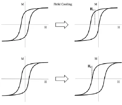
the material shows an increased coercivity, i.e. a widening of the hysteresis loop. Both these effects, schematically shown in Figure 2.6, disappear as the measuring temperature approaches to the AFM Néel temperature.

Figure 2.6 Schematic representation of the two main effects induced by the

AFM-FM exchange coupling, the loop shift (top) and coercivity enhancement (bottom).27

This behaviour can be rationalized considering that exchange biased nanostructures exhibit a new type of induced unidirectional anisotropy (Kud), presenting a Kudcos(ϴ) angular dependence.

As can be seen in Figure 2.7 the energy of a system with uniaxial anisotropy presents two stable positions at 0° and 180°, while the exchange bias induced anisotropy produces a unique minimum at 0°. The uniaxial contribute is the dominant one while the exchange acts as perturbative term of the total anisotropy and its effect is to make the two minima no more equivalent and the cycle loses symmetry.

Figure 2.7 Change from uniaxial (left) to unidirectional anisotropy (right); solid

lines represent torque (sin(ϴ)) and dashed ones the global magnetic energy (sin2_(ϴ)).27

Even if the cause of exchange bias in nanoparticles is still not completely understood, usually the observed unidirectional anisotropy and the loop shift are explained in terms of parallel alignment of the interfacial FM and AFM uncompensated spins occurring during the field cooling process.26,27

Figure 2.8 Schematic diagram of the spin configurations of a FM–AFM couple

before and after the field cooling procedure.27

if a magnetic field is applied, all the spins on the FM are aligned in the same direction of the external field (H), and also the spins of the AFM are partially or totally oriented with the field, since T >TN (paramagnetic

state). When the temperature decreases below TN the spins of the AFM

align antiparallel to each other with the interfacial layer parallel to the FM and thus to H.

This exchange coupling entails an extra energy barrier for FM spin to reverse leading the system to behave as show in Figure 2.9.

Figure 2.9 Schematic diagram of magnetic behaviour during a hysteresis loops

for a AFM-FM spins system with large KAFM (left) and with small KAFM (right).27

After the field cooled procedure, the spins in both the FM and the AFM lie parallel to each other at the interface, and during the demagnetizing process two different situations can occur depending on the anisotropy constant of the two phases. If KAFM ≫ KFM, the FM starts reversing its

magnetization and the exchange-coupling interaction with the AFM, whose spins remain pinned in the original direction, increases the coercive value at negative fields. Conversely, during the magnetization process from negative saturation, exchange-coupling interaction with AFM promotes the magnetization reversal in the direction of the cooling field

decreasing the coercive value at positive field. As a result, the hysteresis loop shifts to the left in the field axis and it is now centred in HE instead

that on the origin. On the other hand, if KAFM ≤ KFM, the two phases reverse

their magnetization together. Then, the energy needed to switch FM spins becomes larger in both branches of the hysteresis loop, since the FM must drag AFM spins. Therefore, the final loop shows an enhancement of both coercive fields.

Assuming the FM and AFM easy axes are parallel and the magnetization rotates coherently, the energy per unit surface in the AFM-FM exchange coupled system can be expressed as:

𝐸

𝑆 = −𝐻𝑀𝐹𝑀𝑡𝐹𝑀cos(𝜃 − 𝛽) + 𝐾𝐹𝑀𝑡𝐹𝑀𝑠𝑖𝑛

2_{(𝛽) +}

𝐾_𝐴𝐹𝑀𝑡_𝐴𝐹𝑀𝑐𝑜𝑠2_{(𝛼) − 𝐽}

𝐼𝑁𝑇cos(𝛽 − 𝛼) (2.15)

where H is the applied magnetic field, MFM is the saturation magnetization

in the FM, tFM and tAFM are the thicknesses of the FM and AFM layers,

respectively, KFM and KAFM are the magnetic anisotropies and JINT is the

exchange coupling constant at the interface. The angles α, β and θ are the angles between the spins in the AFM and the AFM easy axis, the direction of the spins in the FM and the FM easy axis and the direction of H and the FM easy axis, respectively. As can be seen from the different energy terms, if no coupling exists between the two phases and H is turned off, the overall energy of the AFM-FM system reduces to the terms due to the FM and the AFM magnetic anisotropies (2nd and 3rd terms). When a magnetic field is applied, a work has to be carried out to rotate the spins in the FM (1st term). Finally, the 4th term represents the AFM-FM coupling.

In the case the AFM has a very large anisotropy and its spins remain pinned along the field cooling direction and do not rotate with the field (α

= 0), the horizontal shift obtained for the hysteresis loop is given by

𝐻𝐸 =

𝐽_𝐼𝑁𝑇 𝑀𝐹𝑀𝑡𝐹𝑀

(2.16)

Conversely, for low values of the AFM anisotropy the rotation of both the FM and AFM spins is more energetically favourable, and no horizontal shift is induced. However, since the overall anisotropy of the system is changed, an increase of the coercivity is induced.25,28

In Equation 2.16, the HE value is slightly overestimated due to the

assumption to have homogeneous layers in the x-y plane, sharp interface, coherent magnetization reversal and parallel uncompensated spins of both phases. To overcome this issue, more complex approaches accounting for lateral magnetic structures of the layer, interface roughness and different spin configuration, have been developed.26,27,29

Even if the Equation 2.16 describes an ideal system, it can be used for drawing some qualitative considerations about which strategies can be followed to maximize HE: since it is inversely proportional to the FM

thickness, small tFM and strong phase coupling, favoured by epitaxial

interface relationship, are required. Also, the dependence of HC on tFM

follows a similar trend, increasing as tFM decreases. More complicated is

the dependence of HE on the AFM thickness (tAFM). For thick AFM layers,

e.g. over 20 nm, HE is independent of the thickness of the AFM layer.

Conversely, if the AFM thickness is reduced, HE decreases abruptly and

finally, for thin enough AFM layers (usually few nm), when KAFMtAFM <

thickness, above which HE disappears and HC drops to the value of the

uncoupled FM, with the following equation:27

𝑡_𝐴𝐹𝑀𝑐𝑟𝑖𝑡. = 𝐽𝐼𝑁𝑇

𝐾_𝐴𝐹𝑀 (2.17)

The theory of exchange bias systems assumes that TC > TN, however, it

has been extensively proved that exchange bias also occurs in inverted systems where TC < TN.30,31,32,33 It was observed that the HE induced in

these systems can persist also into the PM state of the FM (T > TC) and

close to TN, due to the moments of the FM layer at the interface which are

polarized by the magnetic field. Under certain conditions, these polarized moments couple with the AFM leading to the exchange bias properties.32,33

2.6 Synthesis of magnetic nanoparticles

The vast technological interest of magnetic nanoparticles has fuelled in the last decades an intense research aimed at developing magnetic system with controlled size, shape, composition, etc. The many methods developed so far to produce magnetic nanoparticles can be grouped in two classes: those based on the “top-down” approach, which employs physical methods for the size reduction of bulk materials (i.e. milling or attrition), and those relying on the “bottom-up” approach (i.e. colloidal chemical synthesis, chemical vapor deposition, combustion), where nanostructures are grown starting from constituent atoms or molecules.34,35,36,37 The main advantage of the top-down approach is the possibility to yield a large amount of material, although often the synthesis of uniform-sized nanoparticles and their size and shape control is very difficult to be achieved. The bottom-up

approach allows for obtaining nanoparticles with controlled size distribution, despite generally only sub-gram quantities can be produced. The aim of this work is to synthetize hybrid complex nanostructure with different materials and various-shaped nanoparticles, thus, with this purpose a bottom-up colloidal chemical synthesis approach was used for nanoparticles preparation. This comprises several different techniques, both occurring in liquid (e.g., co-precipitation, microemulsion, thermal decomposition, etc.), gas (chemical vapour deposition, arc discharge, laser pyrolysis) or solid phases (combustion, annealing)38. Thanks to their versatility, control on size and size-distribution and purity of the obtained materials, liquid phase syntheses are the most popular strategies.39,40 In this work thermal decomposition in high boiling solvent technique has been chosen for the synthesis of the entire series of the presented materials. This technique was selected since it grants high control on size, size-distribution, shape, composition and crystallinity. Moreover, since we need to finely tuning the chemical physical properties of the final products, a lot of efforts were devoted to investigating the role of each synthetic parameters in determining the physical characteristic of th final products. Therefore, in the following paragraph the principles of the thermal decomposition technique are briefly reported.

2.7 The thermal decomposition technique

Highly monodispersed nanoparticles with a good control on size and shape can be obtained by high-temperature decomposition of organometallic precursors as metal-acetylacetonate, metal-carbonyl, metal complex with fatty acids conjugate base, etc. in organic solvents. The synthesis takes

place in the presence of surfactants (e.g., oleic acid, oleylamine, lauric acid, 1,2-hexadecanediol, etc.) that act both as stabilizing agents for the obtained nanoparticles and as reagent for the formation of reaction intermediates in the synthesis process. Thermal decomposition of organometallic precursors where the metal is in the zero-valent oxidation state (e.g., metal-carbonyl) initially leads to the formation of metal nanoparticles that, if followed by an oxidation step, can lead to high quality monodispersed metal oxides.41 The decomposition of precursors with cationic metal centres (e.g., metal- acetylacetonate or metal-oleate) leads directly to metal oxides nanoparticles.40 Several synthesis parameters such as precursor concentration, metal-to-surfactant ratio, type of surfactant and solvent are decisive for controlling the composition, size and morphology of the obtained nanoparticles. Moreover, the reaction temperature and time, the heating rate as well as the aging period may also be crucial for the precise control of size, morphology and crystal phase.42,41 It is important to underline that all these synthetic parameters are mutually dependent, which makes the full definition of the reaction mechanism a hard task to eb achieved. Indeed, despite of the many studies reported in literature to date, the full understanding of the reaction mechanism has not been realized. Nevertheless, based on the nucleation and growth theory and on the large number of experimental data reported in the literature, some general consideration about the role of the main synthetic parameters can be provided. The synthetic process starts with the thermal decomposition of the metal-organic precursor which leads to the supersaturation condition, followed by the formation of metal nuclei (nucleation step) and their growth (growth step) leading to metal nanoparticles of different size and shape.

As reported in figure 2.10, a high temperature during the nucleation process (T1) will promote the formation of a high number of nuclei, while

an increase in the temperature during the growth stage (T2) results in an

enhancement of dissolution of smaller nanoparticles. Hence, the setting of high T1 or T2 in the heating procedure will produce smaller or larger

nanoparticles, respectively. Thus, the final particle size is strongly affected by the choice of the solvent, whose boiling point determines the highest exploitable T2.43

Figure 2.10 Schematic description of the heating ramp used in the thermal

decomposition synthesis1_.

A crucial role is played by the reaction time which can be varied: with long growth time (t2), larger nanoparticle size is obtained while the

size-distribution decreases due to the extended focusing region. On the other hand, a short nucleation time (t1) limits heterogeneous nucleation. Thus, in

order to synthetized nanoparticles with small size-distribution it is appropriate to set short t1 and long t2.43

The type of surfactant used in the synthetic process is another crucial parameter in the synthesis. Murray et al.45 demonstrated that the surfactant strongly affects both monomer reactivity and particle surface energy, controlling, thus, the entire crystal growth.44,45 During the synthesis, indeed, the surfactant is involved both in the nucleation process, forming an intermediate complex with the precursor, and in the growth stage, where it acts as stabilizing agent preventing nanoparticles agglomeration. Therefore, if the surfactant and precursor interaction becomes stronger, the intermediate reactivity will be lower and higher T1 and T2 are necessary

for nucleation and growth processes, and vice versa. Similarly, the strength of the surfactants and particles surface interaction can affect the growth stage.45,46 Moreover, exploiting the different affinity of surfactants for different crystallographic faces, it is also possible to tune nanoparticle shape. Particularly, the effect of surfactant depends both on its polar part, (oxygen or nitrogen determine stronger or weaker interaction with precursors or particle surface), and on the hydrophobic chain, (longer chains increase intermediate stability and decrease surface energy of the particles).

References

1 E. Lottini, PhD thesis, 2016, 145.

2 R. Prozorov, Y. Yeshurun, T. Prozorov and A. Gedanken, Phys.

Rev. B - Condens. Matter Mater. Phys., 1999, 59, 6956–6965.

3 E. C. Stoner and E. P. Wohlfarth, Philos. Trans. R. Soc. London.

Ser. A, Math. Phys. Sci., 1948, 240, 599–642.

4 M. Knobel, W. C. Nunes, L. M. Socolovsky, E. De Biasi, J. M. Vargas and J. C. Denardin, J. Nanosci. Nanotechnol., 2008, 8, 2836–2857.

5 D. L. Leslie-Pelecky and R. D. Rieke, Chem. Mater., 1996, 8, 1770–1783.

6 C. P. Bean and J. D. Livingston, J. Appl. Phys., 1959, 30, S120– S129.

7 X. Batlle and A. Labarta, J. Phys. D. Appl. Phys., 2002, 35, R15-R42.

8 S. Shtrikman and E. P. Wohlfarth, Phys. Lett. A, 1981, 85, 467– 470.

9 M. Knobel, W. C. Nunes, A. L. Brandl, J. M. Vargas, L. M. Socolovsky and D. Zanchet, Phys. B Condens. Matter, 2004, 354, 80–87.

10 J. L. Dormann, D. Fiorani and E. Tronc, J. Magn. Magn. Mater., 1999, 202, 251–267.

11 J. L. Dormann, L. Bessais and D. Fiorani, J. Phys. C Solid State

12 W. Luo, S. R. Nagel, T. F. Rosenbaum and R. E. Rosensweig, 1991, 67, 2721–2724.

13 M. Sasaki, P. E. Jönsson, H. Takayama and P. Nordblad, Phys.

Rev. Lett., 2004, 93, 139701–1.

14 S. Mørup and E. Tronc, 1994, 72, 3278–3281.

15 D. Kechrakos and K. Trohidou, Phys. Rev. B - Condens. Matter

Mater. Phys., 1998, 58, 12169–12177.

16 K. Trohidou and M. Vasilakaki, Acta Phys. Pol. A, 2010, 117, 374–378.

17 S. Gangopadhyay, G. C. Hadjipanayis, C. M. Sorensen and K. J. Klabunde, IEEE Trans. Magn., 1993, 29, 2619–2621.

18 A. Lyberatos, 1986, 59, 1–4.

19 D. Kechrakos, K. N. Trohidou and M. Vasilakaki, J. Magn. Magn.

Mater., 2007, 316, 291–294.

20 S. Mørup, M. F. Hansen and C. Frandsen, Beilstein J.

Nanotechnol., 2010, 1, 182–190.

21 M. F. Hansen and S. Mørup, J. Magn. Magn. Mater., 1998, 184, L262-274.

22 E. F. Kneller and R. Hawig, IEEE Trans. Magn., 1991, 27, 3588– 3600.

23 E. E. Fullerton, J. S. Jiang and S. D. Bader, 1999, 200, 392–404. 24 E. H. Frei, S. Shtrikman and D. Treves, Phys. Rev., 1957, 106,

25 W. H. Meiklejohn and C. P. Bean, Phys. Rev., 1956, 102, 1413– 1414.

26 J. Nogués and I. K. Schuller, J. Magn. Magn. Mater., 1999, 192, 203–232.

27 J. Nogués, J. Sort, V. Langlais, V. Skumryev, S. Suriñach, J. S. Muñoz and M. D. Baró, Phys. Rep., 2005, 422, 65–117.

28 W. H. Meiklejohn, J. Appl. Phys., 1962, 33, 1328–1335. 29 M. Kiwi, J. Magn. Magn. Mater., 2001, 234, 584–595.

30 J. W. Cai, K. Liu and C. L. Chien, Phys. Rev. B - Condens. Matter

Mater. Phys., 1999, 60, 72–75.

31 X. W. Wu and C. L. Chien, Phys. Rev. Lett., 1998, 81, 2795–2798. 32 M. G. Blamire, M. Ali, C. W. Leung, C. H. Marrows and B. J.

Hickey, Phys. Rev. Lett., 2007, 98, 1–4.

33 K. D. Sossmeier, L. G. Pereira, J. E. Schmidt and J. Geshev, J.

Appl. Phys., 2011, 109, 1-5

34 A. L. Rogach, D. V. Talapin, E. V. Shevchenko, A. Kornowski, M. Haase and H. Weller, Adv. Funct. Mater., 2002, 12, 653–664. 35 T. Hyeon, Chem. Commun., 2003, 3, 927–934.

36 G. Schmid, Wiley-VCH Verlag GmbH & Co., 2004.

37 K. J. Klabunde, Nanoscale Materials in Chemistry, New York, 2001.