Department of Physics and Earth Science
Ph.D. in Physics
Modeling the Heavy-Ion Collisions with
ECHO-QGP: a novel resource for the study of
the QGP
Co-Advisor
Giuseppe Pagliara Student
Advisor Valentina Rolando
Alessandro Drago
2012-2015 – XXVII course Coord. Prof. V.Guidi – FIS/04
Department of Physics and Earth Science
Ph.D. in Physics
Modeling the Heavy-Ion Collisions with
ECHO-QGP: a novel resource for the study of
the QGP
Co-Advisor
Giuseppe Pagliara Student
Advisor Valentina Rolando
Alessandro Drago
2012-2015 – XXVII course Coord. Prof. V.Guidi – FIS/04
Contents
Introduction 2
0.1 Investigating the Quark Gluon Plasma phase . . . 2
0.2 Historical overview and hydrodynamics achievements . . . . 4
0.3 ECHO-QGP . . . 6
0.4 Outline . . . 8
1 Relativistic Viscous Hydrodynamics 10 1.1 Ideal Hydrodynamics . . . 10
1.2 Dissipative Hydrodynamics . . . 13
1.3 Hydrodynamics in ECHO-QGP . . . 17
1.3.1 Formalism in ECHO-QGP . . . 17
1.3.2 Implementation in ECHO-QGP . . . 19
1.4 Validation of the ECHO-QGP . . . 23
1.4.1 Mildly relativistic 1D shear flow . . . 23
1.4.2 2D shock tubes . . . 24
1.4.3 Boost invariant expansion along z-axis . . . 25
1.4.4 2+1D tests with azimuthal symmetry . . . 28
1.4.5 3+1D test in Minkowski . . . 33
2 Numerical Set-Up, Features and results of ECHO-QGP 35 2.1 Initial conditions . . . 35
2.1.1 MC-Glauber initial conditions: a test case . . . 38
2.2 Equation of State . . . 40
2.3 Decoupling stage . . . 43
2.3.1 Particle spectra in presence of dissipation . . . 46
3 A study of vorticity formation in Heavy-ion collisions 62
3.1 Vorticities in relativistic hydrodynamics . . . 63
3.1.1 The kinematical vorticity . . . 63
3.1.2 The T-vorticity . . . 64
3.1.3 The thermal vorticity . . . 65
3.2 Vorticity in high energy nuclear collisions . . . 67
3.3 Vorticities in ECHO-QGP: novel tests . . . 70
3.3.1 T-vorticity for an ideal fluid . . . 71
3.3.2 T-vorticity for a viscous fluid . . . 72
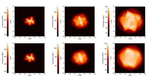
3.4 Directed flow, angular momentum and thermal vorticity . . 73
3.5 Polarization . . . 78
3.6 Plausibility of the initial conditions for the angular momentum 82 4 A perturbative approach to the hydrodynamics of heavy-ion collisheavy-ions 84 4.1 Theoretical basis . . . 85
4.2 Single mode . . . 87
4.3 Higher harmonics . . . 91
4.4 Application to realistic initial conditions . . . 93
Conclusions and Outlook 97
Appendices 102
0.1
Investigating the Quark Gluon Plasma phase
Despite the solid theoretical basis of Quantum Cromo-Dynamics (QCD), the QCD phase diagram (see a sketch of it in fig. 1, and a complete review in ref [1]) is still not fully theoretically understood. This descends from the extreme complexity of the QCD calculations (strong coupling), finding an exact solution is hard enough to push physicists towards approximate methods, each one with a validity window restricted to particular areas of the phase diagram.
QCD features an important property: its coupling constant runs towards
Temperature [MeV]
Critical Point? Critical Point?QGP phase
QGP phase
Net baryon density n/n
0early universe LQCDLQCD 100 200 chiral transit ion deconfinement transition Quarkyonic Phase Quarkyonic Phase Color Super Conductivity? neutron stars neutron stars L C H L C H RH IC RH IC NICA -MPD NIC A-MPD F AIR-SIS F AIR-SIS nuclei
hadronic
phase
Figure 1: Cartoon representation the QCD phase diagram. The strongly interacting quark matter is known to have different phases, due to the unique features of QCD. In this work we will mainly focus on the high temperature and low density region.
asymptotic freedom. This leads to the natural anticipation that QCD matter at high energy densities undergoes a phase transition from the hadronic phase, at low temperature and chemical potential, into a new state of matter with deconfined quarks and gluons. The latter is known as the Quark Gluon Plasma (QGP) phase.
The QGP phase is still experimentally widely unknown, and theoret-ically firm statements about its properties can be made only in limited cases – at finite temperature with small baryon density (µB ≪ T ) and that at asymptotically high density (µB ≫ ΛQCD). In particular, standard
Monte Carlo techniques used in lattice QCD calculations show that at vanishing baryon density, the transition between the hadron phase and the QGP phase is actually a crossover [2]. Due to the the sign problem posed by finite density, standard Monte Carlo techniques used in lattice QCD fail at finite values of the chemical potential, so lattice QCD is less effective to explore the QCD phase diagram moving away from vanishing baryon density (see for instance [3]). In such area of the phase diagram, we can find experimental results descending from ultra-relativistic heavy-ion collisions experiments, which artificially reproduced for the first time the QGP, which is considered to have filled the early universe up to times of 10−5− 10−4 s (hence the name “little bangs” [4, 5]).
The investigations devoted to the modelization of the heavy-ion colli-sions, pushed by the experiments started a couple of decades ago and still ongoing, gave birth among other theories to the hydrodynamic modeling of the collision, whose purpose is to dynamically represent the phase transition (see a chronological summary in [6]).
Experiments, started a couple of decades ago and still ongoing, showed evidence of the presence of the QGP phase. Since the plasma evolves on a strong interaction time scale, the community was motivated to develop theoretical schemes to model the dynamics of the phase transition from the QGP to the hadronic phase. One of the most successful framework is the hydrodynamic approach to heavy-ion collisions.
0.2
Historical overview and hydrodynamics
achieve-ments
While the very first hint that the collision between heavy particles, like atomic nuclei, can be modeled exploiting collective theories like fluid-dynamics dates back to the 1950s [7], this approach really had a boost in the scientific community at the end of the 1970s. The main sources of the interest toward these models were the ongoing experiments, which covered a range of energy in the center of mass from a few hundred MeV (Berkeley LBNL) up to 5 GeV (AGS at BNL) and 17 GeV (SPS at CERN) per nucleon [8, 9]. Even if it was not obvious that a new state of matter had been obtained, the results of such fixed-target experiments showed the presence of collective behaviour, and in particular that the medium undergoes a collective expansion in the plane perpendicular to the beam [10]. The flat behaviour of the particle spectra around mid-rapidity led Bjorken [11] to propose the simplified model of a ultra-relativistic fluid expanding radially in a boost-invariant space. Even if this model failed to describe the transverse collective behaviour, it cast the basis of the hydrodynamic approach to heavy-ion collisions.
In particular, in the decades from 1980 to 2000, a lot of effort went into the development of codes that solved the equations of motions for a relativistic ideal fluid in one and two transverse directions (e.g. [12–14]), motivated by the experimental evidence of transverse flow [15, 16] and in particular of elliptic flow [17], which is an anisotropic emission around the beam direction due to the difference of pressure gradients along the axes of the transverse plane.
Applying a collective theory such as ideal hydrodynamics in a regime of strong coupled interactions was something daring, but it turned out that numerical models could qualitatively predict the behaviour of all low transverse momentum (i.e. soft ) observables produced in heavy ions collisions. The quantitative comparison among the theory and the data though, showed a sharp discrepancy: although the particle spectrum was correctly reproduced in the low transverse momentum region, the elliptic flow was overestimated by about 50% [18]. In the same years, microscopic approaches based on a kinetic description of systems of scattering hadrons were also developed and correctly predicted the elliptic flow [19]; but the same kinetic approach, taken alone, failed in the subsequent years at higher energies [20, 21].
or lead nuclei up to energies in the center of mass of sNN = 130 GeV
and √sNN = 200 GeV per nucleon. These experiments brought conclusive
evidence of the expected new phase state of the matter, called Quark Gluon Plasma (QGP), in which hadrons melt into deconfined colored degrees of freedom, quarks and gluons, predicted by QCD. This evidence also involved a huge drop in the net baryon distribution as a function of the rapidity in the most central collisions (see [22] and figure 3 therein), showing a medium transparent to nuclear collision, which reflects the presence of the hot medium together with the absence of nuclei fragments and indicating the creation of the QGP (this process is also known as baryon stopping). To further corroborate the evidence, the so called jet quenching was observed for the first time, a process that involves the suppression of the momentum of mini jets of hadrons passing through the bulk.
For the first time hydrodynamics could be quantitatively compared to experiments [23], and this induced many in the scientific community to claim that the QGP is a “nearly perfect fluid”: due to the asymptotic freedom in QCD and the color Debye screening, the QGP was expected to behave like gas and produce no anisotropy in the momentum flow . Instead, given the agreement with hydrodynamics, the idea of a strongly coupled plasma flowing as a perfect liquid spread among the community [24–26].
In the next years the applicability of hydrodynamics was questioned, and in fact it appeared that the initial success of ideal fluid dynamics was in reality tainted by the use of a non-realistic equation of state for the fireball (see [27]) together with a treatment of its chemical composition which did not properly reflects its late hadronic stage [28].
In particular some works [29–32] restricted the region in which hydro-dynamics is effective to the (early) QGP phase, in which the fluid has undergone low dissipative effects. Since the late hadronic stage is bet-ter represented by microscopic theories, various hybrid approaches were proposed, in which the description switched from hydrodynamic to ki-netic. The presence of dissipative effects draw anyway the attention to the possibility of a viscous QGP phase description [31, 33–36]. In fact with experiments giving more and more refined results it became evident the need of a (although small) viscosity even in the most central collisions. Further studies, motivated by the need to give a precise and quantitative description of the QGP phase, brought to the community more and more accurate hydrodynamic numerical codes, testing their ability to handle extreme regimes, extending the model to a full (3+1)-D space and including
viscous corrections to higher orders [37–42].
0.3
ECHO-QGP
In spite of the huge progress due to the new experimental discoveries and theoretical advances made over the past decades, several open questions regarding the nature, structure and origin of the QGP are still debated. It has still to be understood what is the smallest size and density for a system of QCD matter to conserve the liquid behavior [43]; what are the transport properties of the QGP and how they are affected by its chemical composition; how its collective properties emerge from the interactions among the individual quarks and gluons and what is the precise nature of the initial state; how it reaches in such a short time an approximate local thermal equilibrium and all the same undergoes such a rapid expansion, whether the applicability of hydrodynamics in a strongly coupled regime is meaningful ... and the open questions are so many that deserve an entire work just to be discussed [44]. Even though the effort towards the understanding of the QGP phase diagram involves the worldwide physic community, and the hydrodynamics is a very well know approach to inves-tigate it, we are still lacking a reliable and widespread resource, accessible to any scientist wanting to approach the open questions. The ECHO-QGP was firstly formed with the goal to provide an answer to this problem.
ECHO-QGP lies among the most refined numerical hydrodynamic codes to describe the QGP phase. It has been built on top of the Eulerian Conservative High Order code for General Relativistic
Magneto-Hydro-Dynamics (GRMHD) [45], originally developed and widely used for high-energy astrophysical applications. ECHO-QGP shares with the original code the conservative (shock-capturing) approach, needed to treat shocks and other hydrodynamical discontinuities that invariably arise due to the intrinsic nonlinear nature of the equations, and the high accuracy methods for time integration, and spatial interpolation and reconstruction routines, needed to capture small-scale fluid features and turbulence. With respect to the original hydrodynamical version of the code, where only the ideal case was treated, ECHO-QGP fully embeds second-order dissipative effects, treated within the Israel-Stewart-Müller theory frame (treated in more detail in chapter 1).
team has brought ECHO-QGP to come known in the international commu-nity as peer with other accomplished hydrodynamic codes1( [37–42,47–66]), creating a state-of-the-art tool in the heavy-ion collisions physics field and it is also suitable for public distribution.
A 3+1D public code is still missing in the physics community. Few public codes are available [13, 14, 34–36], but none of them performs full 3+1D simulations within a viscous theory. We wold like to remark that the vis-cosity, and in particular its magnitude, is still a matter of debate, while it has been proved to be an essential component of the description. Moreover, the full dimensionality of the simulation is also an essential component: hydrodynamic needs complementary modeling concerning the initial condi-tions and the particle production, which can be constrained by the use of the experimental observables. For instance, within a 2+1D simulation we could not study the particle rapidity spectra or the odd harmonics of the flow as functions of the rapidity.
Adapting a hydrodynamics code born for astrophysical applications to a code for the modeling of heavy-ion collisions is a demanding task. The working plan was distributed as follows: Florence’s group was in charge of the implementation of the Israel-Stewart formalism in the hydrodynamic evolution; Turin’s group worked on the initial conditions and the Equation of state; myself with the group of Ferrara were involved in the implementation of the decoupling process, i.e. the only stage of the calculation that produces results to be compared with experiments. The physical observables obviously depend on the initial conditions and on the hydrodynamic fields, therefore I had to actively collaborate with the other two groups during the development and the test of the code. Concerning the applications of ECHO-QGP to physics problems, I calculated the directed flow and the particle polarization in presence of vorticity during the hydrodynamic evolution. Finally, I collaborated with a group of the theoretical division of CERN, for the study of the evolution of initial state fluctuations through a perturbative method.
1
0.4
Outline
This thesis is structured as follows: in chapter 1 the reader can find an overview of the hydrodynamic description, together with the method used to implement it in ECHO-QGP. In the same chapter there is a collection of tests, proving the suitability of ECHO-QGP to model heavy-ion collisions along with its accuracy. In chapter 2, we describe the setup used for ECHO-QGP and we explain in more detail how to construct the initial state and how the final observables are computed. In chapter 3 ECHO-QGP is exploited to study the vorticity formation in high energy nuclear collisions: we will show how thermal vorticity affects the directed flow and its relation with the final state polarization. In particular, we will discuss the detectability of the polarization of the Λ. In chapter 4 we employ a perturbative approach to the initial state to study the fluid dynamic propagation of fluctuations. In the last chapter we draw conlusions about the work performed with ECHO-QGP and we give an outlook about future perspectives.
1
Relativistic Viscous
Hydrodynamics
Hydrodynamics is a theoretical framework which allows the collective description of a strongly interacting many-body system, through ther-modynamic variables defined locally, masking all the microscopic details. Provided that the initial expansion timescale is sufficiently long compared to the transport mean free path, we can in fact exploit thermodynamic concepts like temperature and pressure to describe the system. Hydrodyna-mics applicability has been extensively discussed (see for instance [67, 68]) but this theoretical frame is currently one of the best dynamic tools to reproduce the experimental observables.
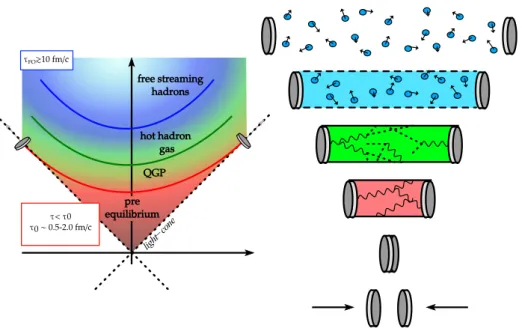
As shown in the cartoon in fig. 1.1, the region in which we apply hydrodynamics is after a pre-equilibrium phase (∼ 1 fm/c), in which the medium achieves local thermal equilibrium, and before the dissipative behavior becomes dominant (and hence better described by a kinetic approach).
In this chapter, we will quickly review the hydrodynamic theory before showing how it is implemented and how it performs in ECHO-QGP.
1.1
Ideal Hydrodynamics
The definition of “Ideal Hydrodynamics” is currently accepted as a synonym of non-viscous. It is anyway important to remark that ideal hydrodynamics does not necessarily imply the global thermodynamic equilibrium: when
light− cone hot hadron gas QGP pre equilibrium free streaming hadrons τ< τ0 τ0 ∼ 0.5-2.0 fm/c τFO≳10 fm/c
Figure 1.1: Cartoon representation of a Heavy-ion collision. The origin of the axis represents the instant of the collision, assuming that the nuclei are moving at the speed of light along the light-cone, where the remnants of the shattered nuclei continue to move. The medium is believed to ther-malize in a time of the order of 1 fm/c. The average life of the fireball is of about 10 fm/c, and in such interval hy-drodynamic is exploited to model its evolution. When the scattering rate of particles is of the order of the expansion rate, hydrodynamics ceases to be applicable.
all transport coefficients are vanishing, there can still be the presence of thermodynamic force with no entropy production.
The hydrodynamic flow (uµ) is denoted as a four velocity with its normalizing condition, which defines the fluid Lorentz factor (γ ≡ u0)
uµ≡ γ(1, vi) uµuµ= −1 γ = (1 − gijvivj)−1/2 vi ≡ ui/γ (1.1)
In ideal hydrodynamics, the system is well and fully described by its energy momentum tensor and the conserved charge current
N0µ= n0uµ (1.2)
T0µν = e0uµuν+ ∆µνP0 (1.3)
where the orthogonal projector operator has been introduced, written as: ∆µν ≡ gµν+ uµuν, (1.4) and it respects the orthogonality relation: ∆µνuµ= 0. The local equilibrium
thermodynamic quantities are defined by the relations
e0 = uµuνT0µν energy density (1.5) P0 = 1 3∆µνT µν 0 hydrostatic pressure (1.6)
n0 = −uµN0µ conserved charge density (1.7)
In case of multiple conserved charges the equation 1.2 must be valid for each conserved charge ni0.
The conservation of the energy-momentum tensor and conserved current are written as:
dµN0µ= 0, (1.8)
dµT0µν = 0. (1.9)
where the covariant derivative (dµ) could be decomposed along its temporal direction D ≡ uαd
α, and along its spatial direction ∇µ≡ ∆µαdα.
dµ= −uµD + ∇µ, (1.10)
Equations 1.8-1.9 provide a set of 4+1 independent equations (or 4+N for N multiple conserved currents) with 5+1 (5+N) independent variables namely: n0, e0, P0, uµ. The set given by the conservation laws alone does
not give a complete description, for this reason an Equation of State (EoS) is usually adopted to close the system, i.e. a relation P0 = P(e0, n0).
1.2
Dissipative Hydrodynamics
The parabolic character of the equation of heat has been recognized as a fallacy due to the unsuitability of conventional thermodynamics in describ-ing transient regimes. In fact, in the Navier-Stokes approach the dissipative quantities react instantaneously to the thermodynamic forces, but the instantaneous propagation implies acausality, for which reason a consistent generalization of the Navier Stokes equations in a relativistic frame is forbidden. Along with the causality violation, the first-order theory has stability problems, having exponentially growing modes when the pertur-bation from global equilibrium is infinitesimally small (see for instance [69]).
Relaxing the instantaneous propagation assumption by introducing characteristic time scales, which regulate the response of the dissipative quantities to the corresponding thermodynamic forces, causality and stabil-ity issues are removed and the theory becomes stable and causal. While the value and the importance of the higher order transport coefficients is still a hot topic ( [70, 71]) historically, the first second-order theory approach for viscous hydrodynamics was proposed by Israel and Stewart [72].
In 1949 Grad proposes a new theoretical approach in the framework of the classical kinetic theory, appliyng a method of moments (now known as Grad-14 moments approximation) and obtaining the set of classical dissipative fluid-dynamics equations [73]. In 1967 [74] Müller presents a phenomenological derivation of the non relativistic thermodynamics, includ-ing second order terms in heat flow and viscosity conventionally neglected, which is consisitent with Grad’s kinetic approach. In 1970 Stewart [75] elaborates the relativistic extension of the Grad’s approximation, along with others (Anderson and Stewart [76], Marle [77], Kranys [78–81]). In 1976 Israel extends the phenomenological approach to the relativistic case. In 1987 the comprehensive work of Israel and Stewart [72] draws together the collection of all kinetic and phenomenological approaches, providing the explicit form of the transport coefficients in the generalized transport equations for a relativistic quantum gas.
In this work a second-order Israel-Stewart treatment has been used and implemented in ECHO-QGP. The energy-momentum tensor and the conserved currents are decomposed as
Nµ= nuµ+ Vµ, (1.11)
Tµν = euµuν+ (P + Π)∆µν+ πµν+ wµuν+ wνuµ, (1.12) where the viscous contributions to the energy momentum tensor are respec-tively the shear (πµν) and bulk part Π of the viscous stress tensor. The following definitions do apply:
conserved charge density n = uµNµ (1.13)
particle diffusion flux Vµ= ∆µαNα (1.14) energy density e = uµuνTµν (1.15)
isotropic pressure P + Π = 1 3∆µνT
µν (1.16)
energy-momentum flow orthogonal to uµ wµ= −∆µαTαβuβ (1.17)
where the shear component of the stress tensor is defined as
πµν = [12(∆µα∆νβ+ ∆µβ∆να) −13∆µν∆αβ]Tαβ (1.18)
and satisfies the orthogonality and traceless requirements:
πµνuν = 0 (1.19)
πµµ= 0. (1.20) When the dissipative quantities vanish (Vµ= wµ= πµν = Π = 0), we recover the ideal decompositions N0µ= n0uµ and T0µν = e0uµuν+ P0∆µν.
To guarantee the thermodynamic stability of the system, in the local rest frame of the fluid (LRF), the quantities n and e are fixed to their equilibrium values by utilizing the Landau matching conditions (n = n0, e = e0). The pressure is recovered using an appropriate equation of state
(EoS) as P = P(e, n) = 13∆µνT0µν.
When treating the theory up to orders higher than the first, one loses the equivalence between the four-velocity parallel to Nµand the normalized timelike eigenvector of Tµν, which were equivalent in the first order theory. In principle any frame that arbitrarily deviates from the equilibrium frame is a valid choice for the hydrodynamic flow, since the only condition that has to be fulfilled is that the dissipative components of the conserved
quantities are small compared to the equilibrium ones. The two most common possibilities for the selection of the frame are the Landau frame in which there is no net energy-momentum flow (wµ= 0); or the Eckart frame in which the charge dissipative flow vanishes (Vµ= 0). The former choice
is the one we adopted in our works, for several reasons. The QGP in High Energy collisions (RHIC, LHC) is created with an extremely small baryon density, letting the equation of state assume the form P = P(e). That is the very case of many hydrodynamic studies and the Landau frame is preferred because the particle frame cannot be defined for the systems with vanishing conserved currents, while the energy frame is always definable. The same argument applies when there are multiple conserved currents: there is no further simplification if other currents are still present, when choosing one of them to vanish.
For vanishing baryon densities we have only one quantity left to describe the dynamics of the fluid and the equation for Nµ becomes redundant in the conservation laws:
dµNµ= 0, (1.21)
dµTµν = 0. (1.22)
It is now convenient to decompose the conservation law of eq.(1.22) along uµ and orthogonal to uµ, in order to derive the energy and momen-tum equations, respectively. In order to do so, one can take advantage of some useful kinematic quantities. The covariant derivative of the fluid velocity can be decomposed in its irreducible tensorial parts, respectively the transverse, traceless, and symmetric component σµν, the
trans-verse, traceless, and anti-symmetric component ωµν and the scalar component θ:
dµuν = σµν+ ωµν− uµDuν+13∆µνθ, (1.23)
where the following definitions apply:
shear tensor σµν = 12(∇µuν+ ∇νuµ) −13∆µνθ, (1.24)
= 12(dµuν + dνuµ) +12(uµDuν+ uνDuµ) −13∆µνθ,
vorticity tensor ωµν = 12(∇µuν− ∇νuµ) (1.25)
= 12(dµuν − dνuµ) +12(uµDuν− uνDuµ),
With the above decompositions, the relativistic energy and momentum equations in 1.22 can be written as
De + (e + P + Π)θ + πµνσµν = 0, (1.27)
(e + P + Π)Duν + ∇ν(P + Π) + ∆νβ∇απαβ+ Duµπµν = 0, (1.28)
where the latter is clearly orthogonal to uν.
Matching fluid dynamics to the underlying microscopic theory (i.e. in the case of dilute gases the Boltzmann equation) is done in the Israel Stewart formalism, through Grad’s method of moments, truncating the expansion at second order in momentum. The coefficients of the truncated expansion can then be uniquely related to the fluid dynamic fields using a matching procedure. The bulk and shear viscous parts of stress tensor, including terms up to second-order in the velocity gradients, satisfy the following evolution equations:
DΠ = −τ1 Π(Π + ζθ) − 4 3Πθ, (1.29) ∆µα∆νβDπαβ= −τ1 π(π µν+2ησµν)−4 3π µνθ−λ(πµλων λ+ πνλω µ λ) (1.30)
(for derivation see for instance [82]). In this analysis, terms that are quadratic in Π, πµν and ωµν are neglected. To obtain the solution of the above evolution equations we shall need to specify the transport coefficients η, ζ, the shear and bulk relaxation times τπ, τΠ, and the other
second-order transport parameter, λ ≡ λ2/η [82]. The parameter λ2 is known
for the weakly coupled, as well strongly coupled N = 4, Super Yang Mills theories [82], but not for the strongly coupled QCD. The vorticity contribution in Eq. (1.30), which contains λ, for the purposes of this chapter will be mostly ignored by letting λ = 0, whereas in specific runs it will be chosen to be 1 as in [83].
Writing explicitly the orthogonal projector as in (1.4) and using orthog-onality condition uµπµν = 0, we can rewrite Eq. (1.30) as
Dπµν = −τ1 π(π µν+ 2ησµν) −4 3π µνθ + Iµν 1 + I µν 2 , (1.31)
where the contributions deriving from the orthogonal projection (I1µν) have been kept apart from the vorticity contribution term (I2µν). They are defined as follows:
I1µν = (πλµuν + πλνuµ)Duλ, (1.32)
1.3
Hydrodynamics in ECHO-QGP
In this section the reader can find a quick summary on how the imple-mentation of the conservation laws (1.21, 1.22) within the ECHO-QGP code.
1.3.1 Formalism in ECHO-QGP
The conservation laws and the evolution equations for the components of Π and πµν must be rewritten in a form suitable for numerical computations: a conservative balance law; in which conserved quantities (U), fluxes (Fi)
and source terms (S) are present:
∂0U + ∇iFi= S (1.34)
In the dissipative case, the system is comprehensive of 13 scalar equations (with the addistion of the equation of state).
Even if the formal setup emplys the Landau frame, it is numerically convenient to evolve the continuity equation in the limit Vµ= 0, in order to improve the stability. Equation 1.21 is rewritten as:
Dn + nθ = 0, (1.35) where the charge density n must be interpreted just as a tracer responding to the evolution of the fluid velocity through the expansion scalar θ. We manipulate the equation to obtain the desired form (1.34)
dµNµ= |g|− 1 2∂µ(|g| 1 2Nµ) = 0, (1.36) or also ∂0(|g| 1 2N0) + ∂k(|g| 1 2Nk) = 0. (1.37)
Again, it is necessary to repeat the same procedure to the conservation of the energy-momentum tensor components 1.22
dµTµν = |g| −1 2∂µ(|g| 1 2Tµ ν) − Γ µ νλT λ µ= 0, (1.38)
where the relation Γµµλ = |g|−12∂λ|g| 1
2, has been employed, in which g is
the determinant of the metric tensor. It is possible to further rewrite this equation making use of the symmetry properties of the energy-momentum
tensor, to obtain: ∂0(|g| 1 2T0 ν) + ∂k(|g| 1 2Tk ν) = |g| 1 2Γµ νλT λ µ = |g| 1 21 2T λµ∂ νgλµ, (1.39)
The adjustment of the evolution laws for the stress tensor component is also needed, to obtain the desired form of balance laws. The previous dµNµ= 0 relation is now useful in order to rewrite the timelike components
of the comoving derivative (D ≡ uµdµ), multiplying the equations for the
evolution of πµν and Π (1.29 and 1.30) by the tracer n, one obtains: ∂0(|g| 1 2N0Π) + ∂k(|g| 1 2NkΠ) = |g| 1 2n − 1 τΠ(Π + ζθ) − 4 3Πθ (1.40) for the evolution of the bulk component of the stress tensor; and
∂0(|g| 1 2N0πµν) + ∂k(|g| 1 2Nkπµν) = |g|12n −τ1 π(π µν+ 2ησµν) −4 3π µνθ + Iµν 0 + I µν 1 + I µν 2 , (1.41) for the evolution of the shear components of the stress tensor. The source terms have been kept non explicit, since they are different for different coordinates systems, but the term I0 has been isolated, since it clearly
vanishes in Minkowski coordinates:
I0µν = −uα(Γµλαπλν+ Γνλαπµλ) (1.42) On the other side, in Bjorken coordinates the non-vanishing I0µν terms are I0xη= −(uτπxη+ uηπτ x)/τ, (1.43) I0yη = −(uτπyη+ uηπτ y)/τ, (1.44) I0ηη = −2(uτπηη+ uηπτ η)/τ, (1.45) while I1µν and I2µν are defined in the usual way.
The technique of introducing the conserved number current as a tracer is exploited in a similar way within a recent code for (2+1)-D Lagrangian hydrodynamics [84] to solve the evolution equation of the bulk viscous pressure Π.
Due to the orthogonality condition, only 6 out of 10 components of the viscous stress tensor are independent. ECHO-QGP can evolve the 5 spatial component πij, or evolve all and only its 6 spatial independent components. The latter choice is the one adopted in the present work, and it generates a system which can be arranged in matrix form to reflect the structure of
1.34, with: conservative variables U = |g|12 N ≡ N0 Si≡ T0i E ≡ −T00 N Π N πij , (1.46) fluxes Fk= |g|12 Nk Tk i −Tk 0 NkΠ Nkπij , (1.47) sources S = |g|12 0 1 2Tµν∂igµν −12Tµν∂0gµν n[−τ1 π(Π + ζθ) − 4 3Πθ] n[−τ1 π(π ij+ 2ησij) −4 3π ijθ + Iij 0 + I ij 1 + I ij 2 ] (1.48)
The above Eqs. 1.46-1.47 together with the eq. 1.34 represent the set of ECHO-QGP equations in the most general form, since ECHO-QGP can work both in Minkowski and Bjorken coordinates.
1.3.2 Implementation in ECHO-QGP
In this section, the reader can find a very brief summary of the numerical techniques used in ECHO-QGP. The name conserved variables is intended for the set of quantities U, explicit in 1.46 entering the equation 1.34, while the expression primitive variables is used to refer to the corresponding physically meaningful quantities, namely: the fluid velocity, the local energy density, the independent components of the shear stress tensor and the charge density (P = {n, vi, P, Π, πij}).
The ECHO-QGP [85] code has been built upon the original ECHO scheme [86] which was, and still is, devoted to relativistic hydrodynamics and MHD (in any GR metric, even time dependent like for Bjorken
coor-dinates) for astrophysics purposes. Therefore, ECHO-QGP shares with ECHO the finite-difference discretization, the conservative approach, and the shock-capturing techniques.
• The spatial grid is discretized along all the directions of interest as a Nx × Ny × Nz set of cells (Nη in Bjorken coordinates). Lower dimensionality runs are always admitted, for example, 2-D tests with boost invariance in Bjorken coordinates are performed by choosing Nη = 1.
• The physical primitive variables set (P = {n, vi, P, Π, πij}) is
initia-lized for t = 0 (or for a chosen τ = τ0in Bjorken coordinates) defining the value of each variable at every cell center.
• During the hydrodynamic evolution, the conservative variables U and fluxes F are calculated at cell interfaces. At first, the corresponding values of the primitive variables are calculated at cell interfaces too. For each “spatial direction”, the primitive variables calculated at the interfaces (i.e. left : PLand right : PR) are used to retrieve the value
at the cell centre.
• For each component and at each intercell, upwind fluxes ˆFk (along
direction k) are worked out using the so-called HLL two-state formula [87] as ˆ Fk = a k +Fk(PL) + ak−Fk(PR) − ak+ak−[U (PR) − U (PL)] ak++ ak− , (1.49)
where the coefficients ak± are calculated as:
ak±= max{0, ±λk±(PL), ±λk±(PR)}, (1.50)
and the local fastest characteristic speeds associated to the Jacobian ∂Fk/∂U, relative to the direction k is calculated as:
λk±= (1 − c2s)vk± c2 s(1 − v2)[(1 − v2c2s)gkk− (1 − c2s)vk 2] 1 − v2c2 s . (1.51) Notice that eq. (1.51), provides an approximated solution to the local Riemann problem. The sound speed is extracted from the Equation
of State: c2s = ∂P ∂e + n e + P ∂P ∂n. (1.52)
• High order derivatives of fluxes are calculated for each direction (corresponding to ∇iFi in eq. 1.34), and then the source terms (S)
are added, leaving the conserved variables (U) be the only unknown. The time derivatives contained in some of the source terms (like in the expansion scalar) are calculated by using their values at the previous timestep.
• The evolution equations are updated in time via a second or third order Runge-Kutta time-stepping routine.
• At each temporal sub-step, the set of primitive variables (P = {n, vi, P, Π, πij}) is calculated starting from the updated set of
cor-responding conservative variables. In order to do so two different methods are exploited: an iterative relaxation method or the more re-fined multidimensional Newton-Raphson root-finding method, which performes the cycle on the vi components. The latter one is the most employed, and it is summarized as follows.
Exploiting the orthogonality conditions πµνuν = 0, one can express
the shear stress tensor components as:
π0i= πijvj, π00= π0ivi= πijvivj, (1.53)
Substituting Si = gijSj and π00= −π00, the conserved variables in
1.46 can be rewritten as
N = nγ, (1.54)
Si = (e + P + Π)γ2vi+ π0i, (1.55) E = (e + P + Π)γ2− (P + Π) + π00. (1.56) The components πij are by all means conserved variables, entitled by the conservation of the charge density, despite its lack of physical meaning in this frame.
Once one has the vi in the Local Rest Frame (LRF), the charge and energy density would be given by:
At this point, the secondary thermodynamic variables can be retrieved through the Equation of State. The best performing technique that was found to calculate the primitive variables is based on an iteration of the method employed in the ideal case, which takes place as an external loop over the vi components and it is closed when a given tolerance in |vnewi − vi| terms is reached. The vi are initialized
with their values at the previous time-step. The cycle performs the following steps:
1. The new quantities ˜E and ˜Si are calculated as:
˜
E = E − π00, S˜i = Si− π0i;
(notice that in the ideal case ˜E ≡ E, ˜Si ≡ Si, ˜P ≡ P so the
external iteration is unnecessary).
2. An inner cycle to retrieve P is performed, which is reiterated until |Pnew− P | reaches the desired tolerance.
(a) In the inner cycle the temporary pressure is calculated, together with the associated primitive variables:
˜
P (P ) = P + Π, v2(P ) = ˜S2/( ˜E + ˜P )2 and
e(P ) = ( ˜E + ˜P )(1 − v2) − ˜P , n(P ) = N1 − v2.
(b) The cycle is iterated via a Newton-Raphson procedure, minimizing the quantity
f (P ) = P[e(P ), n(P )] − P, where f′(P ) = ∂P ∂e de dP + ∂P ∂n dn dP − 1. The updated value of the pressure becomes:
Pnew= P − f (P )/f′(P ),
3. Once retrieved the pressure corresponding to the vi components, their updated value is provided by:
The same procedure can be applied when also the π00and π0iviscous terms were evolved. Thanks to the conservative nature of N , they represent conservative variables, avoiding the necessity of applying the orthogonality condition to extract them.
• The output of primitive variables and other diagnostic quantities are provided for selected output times.
1.4
Validation of the ECHO-QGP
ECHO-QGP has undergone several numerical test, devoted to the evaluation of its response against shocks, of its accuracy in solving equations and its reliability in treating the plasma in extreme conditions. In this section a summary of its performances can be found.
1.4.1 Mildly relativistic 1D shear flow
Assuming a flow that is only mildly relativistic, the diffusion of a shear flow profile in (1+1)D is known analytically. A similar case has already been studied for testing numerical algorithms for relativistic viscosity [88] and also resistive magnetohydrodynamics [45]. This test has been performed in Minkowski coordinates, choosing a velocity profile vy = vy(x). For
sub-relativistic speeds and a uniform background state in terms of energy density and pressure, at any time t of the evolution, only vy will change due to shear viscosity (the bulk viscosity does not play a role since θ ≡ 0), always preserving γ ≈ 1. In such Navier-Stokes limit, the momentum equation along y reads
(e + P )∂tvy+ ∂xπxy = 0, πxy = −2ησxy = −η∂xvy,
which leads, for a constant η coefficient, to the classical 1D diffusion equation
∂tvy = Dη∂x2vy, Dη = η/(e + P ),
with (constant) diffusion coefficient Dη. Assuming a step function for the
vy(x) profile at t = 0, with constant values −v0 for x < 0 and v0 for x > 0,
it is possible to express the exact solution at any time t as:
vy = v0erf 1 2 x2 Dηt .
−1.5 −1.0 −0.5 0.0 0.5 1.0 1.5 x −0.010 −0.005 0.000 0.005 0.010 vy (c units) Analytic ECHO−QGP
Figure 1.2: Comparison between the ECHO-QGP evolution output and the analytic solution at t = 10 fm/c for the dependence of the velocity, in the case of mildly relativistic 1D shear flow. The numerical setup is shown in table 1.1
v0 η Dη Nx [xmin; xmax]
GeV/fm3 fm fm 0.01 0.01 0.01 301 [-1.5,1.5]
Table 1.1: Setup for the mildly relativistic 1D shear flow test. The
chosen EoS is e + P = 4P = 1GeV/fm3. The comparison
with the analytical result is shown in fig. 1.2
In order to proceed to the numerical test, the above profile has been used at the initial time t = 1 fm/c instead of the discountinuous step function, letting ECHO-QGP evolve it up to late times (t = 10 fm/c). The result of such evolution (with the setup described in table 1.1) has then been compared to the analytical solution for the corresponding time (see fig. 1.2), showing perfect agreement.
1.4.2 2D shock tubes
Shock-capturing numerical schemes, as in the classical hydrodynamical case, are designed to handle and evolve discontinuous quantities inevitably arising due to the nonlinear nature of the fluid equations. In order to validate these codes, typical tests are the so-called shock-tube 1D problems.
Nx Ny [xmin; xmax] [ymin; ymax] tend
fm fm fm/c
201 201 [−4; 4] [−4; 4] 4 TL PL TR PR η/s GeV GeV/fm3 GeV GeV/fm3
0.4 5.4 0.2 0.34 0/0.01/0.1
Table 1.2: Setup for the shock tube test, performed with EOS-I (see sec. 2.2) and different values for η/s. The comparison with the analytical result is shown in fig. 1.3
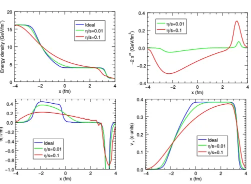
Two uniform states are taken on the left and on the right with respect of an imaginary diaphragm, which is supposed to be initially present and then removed at t = 0. Typical patterns seen in the subsequent evolution are shocks and rarefaction waves. In performing this test, a relativistic blast wave explosion problem is considered, which is characterized by an initial static state with temperature and pressure much higher in the region on the left, namely TL= 0.4 GeV (PL= 5.40 GeV/fm3) and TR= 0.2 GeV (P = 0.34 GeV/fm3). In order to make a more stringent test, the shock-tube test has been performed by placing the initial diaphragm along the diagonal of a square box adopting Minkowskian coordinates 2+1D, and by letting the system evolve in a higher-dimensionality frame from t = 0 up to t = 4 fm/c. The same test has been repeated for the ideal case and for different values of the shear viscosity η/s (0.1 and 0.01). Some of the results of this test, performed within the setup described in table 1.2 are shown in in fig. 1.3, in particular one can find the velocity profile vx, the expansion scalar θ, the energy density e, and the component of
the shear stress tensor −2πzz, as a function of x and along the axis y = 0. As in [71], at the final time (tend = 4 fm/c), ECHO-QGP shows to be free fom numerical spurious oscillations near the shock front even in the ideal (stiffer) case. When introducing the viscosity, profiles are smoother for increasing values of η/s. Small oscillations can be seen in θ (mainly due to the low accuracy in the time derivative) for the largest value of the viscosity.
1.4.3 Boost invariant expansion along z-axis
As a first validation of ECHO-QGP in Bjorken coordinates it was considered a test with no dependence on the transverse coordinates (x, y), implying a vanishing vorticity. For this test, a boost invariance along the z-direction is
Figure 1.3: Hydrodynamic quantities in a relativistic blast wave explosion problem. In this panel there are respectively the
energy density e, the component −2πzzof the shear stress
tensor, the expansion rate θ, and the velocity component
vx, as a function of x for η/s = 0, 0.01, 0.1 at tend =
4 fm/c. The numerical setup is shown in table 1.2
assumed, thus the involved quantities do not depend on ηs either, reducing the dependence of the system to the time coordinate (0+1D test). The evolution of uniform quantities will be then just due to the τ dependence of the gηη term in the metric tensor, in the absence of velocities. The
energy-momentum tensor simplifies to:
Tµν ≡ diag{e, P + Π + πxx, P + Π + πyy, (P + Π)/τ2+ πηη}
where πxx, πyy, and πηη are the only non-vanishing components of the shear stress tensor. Applying to the latter its tracelessness property and exploiting the assumed simmetries, it is possible to write those components as:
2πxx= 2πyy= −τ2πηη≡ ϕ,
so only one independent component of πµν is sufficient to describe the system. Despite this simplification and in order to guarantee the reliability of the code, in this test ECHO-QGP evolves all 6 spatial components
τ0 η/s ζ τπ
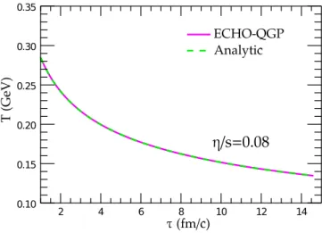
fm/c GeV/fm2 fm/c 1 0.08 0.01 1
Table 1.3: Parameters setup for the boost invariant expansion along z-axis. The comparison with the analytical results is shown in fig. 1.5.
starting at τ = 1 fm/c from a constant initial energy density profile, and never imposing tracelessness. The system as described admits an analytical solution, provided that first-order theory applies. The energy equation is then enough to describe the overall evolution
∂e ∂τ = −
e + P + Π − ϕ
τ . (1.58)
Within the first-order theory, Π and ϕ can be obtained from their Navier-Stokes (NS) values
Π = −ζ
τ, ϕ = 4η 3τ.
Employing the ultrarelativistic gas EoS and assuming constant values for η/s and for ζ/s, eq. (1.58) admits the following analytic solution [89–91] for the temperature as a function of the proper time:
T (τ ) = T0 τ0 τ 13 1 +4η/3s + ζ/s 2τ0T0 1 −τ0 τ 23 ,
where T0 is the temperature at the initial proper time τ0. This last analytic
form is compared with the outcome of ECHO-QGP, set up to reproduce the Navier-Stokes limit. Such comparison can be seen in fig. 1.4 (where ζ/s has been set to 0).
On the other hand, an analytic solution for the evolution equations extracted within the second-order theory has never been derived. However, assuming that the evolution of Π and ϕ is simply governed by the relaxation part of the source terms one can write (τπ= τΠ):
∂Π ∂τ = − 1 τΠ Π +ζ τ −4Π 3τ → ∂Π ∂τ = − 1 τπ Π + ζ τ (1.59) ∂ϕ ∂τ = − 1 τπ ϕ − 4η 3τ − 4ϕ 3τ − τ 2Iηη 1 → ∂ϕ ∂τ = − 1 τπ ϕ − 4η 3τ . (1.60)
2 4 6 8 10 12 14 0.10 0.15 0.20 0.25 0.30 0.35 ECHO-QGP Analytic τ (fm/c) T (GeV) η/s=0.08
Figure 1.4: Comparison between the analytic solution and the same quantity computed numerically by ECHO-QGP of the evolution of the temperature T (τ ) derived in the context of the first-order Navier-Stokes theory (eq. 1.58). Here ζ/s = 0
Assuming η, ζ and τπ to be independent of the temperature, eqs. (1.59,1.60) admit the following semi-analytic solution for Π and ϕ:
Π(τ ) = Π(τ0) e− τ −τ0 τπ + ζ τπ e−τπτ Ei τ0 τπ − Ei τ τπ , (1.61) ϕ(τ ) = ϕ(τ0) e− τ −τ0 τπ − 4η 3τπ e−τπτ Ei τ0 τπ − Ei τ τπ , (1.62) where, Ei(x) denotes the exponential integral function.
The above solutions are obtained from ECHO-QGP under the same assumptions. The comparison between the ECHO-QGP output and the semi-analytic solution for the evolution of Π is shown in fig. 1.5, showing perfect agreement.
1.4.4 2+1D tests with azimuthal symmetry
The study that naturally follows the 0+1D test in Bjorken coordinates, is the boost-invariant case (still ∂η ≡ 0) where one also considers the evolution in
the transverse plane. When the initial state (at τ0) is azimuthally invariant,
the 2+1D evolution with ECHO-QGP can be compared with analytic results in 1+1D.
2 4 6 8 10 12 14 τ (fm/c)
Π
ECHO-QGP Analytic -0.005 -0.004 -0.003 -0.002 -0.001 0.0Figure 1.5: Comparison between the analytic solution and the same quantity computed numerically by ECHO-QGP of the evolution of the bulk viscosity Π(τ ) for the second-order derivation (see eq. 1.61). The numerical parameters setup can be found in tab. 1.3.
the first one assumes a Woods-Saxon initial profile for the energy density and a viscous free evolution [12]; the second and the third ones are an analytical solution (under the assumption of cold plasma) [92] and a semi-analytical solution (less stringent assumptions) of the viscous equations of motions starting from an azhimuthally symmetric initial profile created ad-hoc [68, 93, 94].
Baym’s solution for a Woods-Saxon profile initialization
For the first case, it is assumed a Woods-Saxon profile for the initial energy density, as appropriate for central nucleus-nucleus collisions:
e(r, τ0) =
e0
1 + exp [(r − R)/σ],
where τ0 is the initial time, r = (x2+ y2)1/2 is the radius in the transverse
plane, and R can be thought of as the radius of the nuclei. The analytical solution for the subsequent evolution, as a function of τ and r, was found in ref. [12] and it has been be compared with ECHO-QGP numerical results, with the setup described in table 1.4. As shown in Fig. 1.6, there is a perfect agreement between the analytic solution and ECHO-QGP, at any proper time τ during the evolution.
0 2 4 6 r (fm) T (GeV) 0.00 0.05 0.10 0.15 0.20 τ=4 fm/c τ=7 fm/c ECHO-QGP Analytic τ=2 fm/c 0 2 4 6 0.0 0.2 0.4 0.6 0.8 1.0 τ=7 fm/c τ=4 fm/c τ=2 fm/c ECHO-QGP Analytic vr ( c un its) r (fm)
Figure 1.6: Spatial dependence of the temperature and of the radial velocity at different times along with the analytic solu-tion in the case of a Woods-Saxon initial condisolu-tion with cylindrical symmetry. Results obtained with ECHO-QGP in 2+1D agree very well with the analytical solution by Baym et al. [12].
R r σ T0
fm fm fm GeV 6.4 0 0.02 0.2
Table 1.4: Setup for the 2+1D test (see sec. 1.4.4) with azimuthal sym-metry and boost invariance, performed with a Woods-Saxon initial condition for the energy density profile. Results are shown in fig. 1.6
Gubser flow
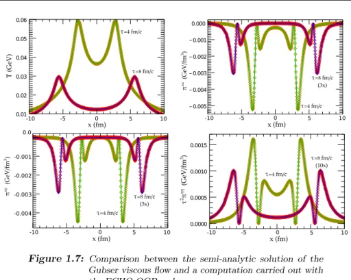
A very useful test for a numerical code of relativistic dissipative hydro-dynamics is the extension of the ideal solution found by Gubser and Yarom [92, 95], in the case of a Bjorken flow with an azimuthally symmetric radial expansion, to the viscous case [68, 94]. Indeed, this solution provides a highly non-trivial theoretical benchmark.
For the sake of clarity, the main steps leading to the analytical solution are briefly summarized below, ad then a comparison with the numerical computation is shown in fig. 1.7.
In the case of a conformal fluid, with P = e/3 EoS, the invariance for scale transformations constrains the terms entering the second-order viscous hydrodynamic equations. The additional requests of azimuthal and longitudinal-boost invariance, constrain the solution of the hydrodynamic equations, which has to be invariant under SO(3)q⊗ SO(1, 1) ⊗ Z2
∆x ∆y ∆ηs ∆τ η/s τR q
fm fm fm/c fm−1
0.025 0.025 0.025 0.001 0.2 5η/(e + P ) 1
Table 1.5: Parameters setup for the Gubser test. 1.7
follows (with usual Bjorken coordinates, ηs being the spacetime rapidity):
ds2 = τ2 dτ 2− dr2− r2dϕ2 τ2 − dη 2 s , which can be viewed as a rescaling of the metric tensor:
ds2−→ dˆs2 ≡ ds2/τ2 ⇐⇒ gµν −→ ˆgµν ≡ gµν/τ2.
It can be shown that dˆs2is the invariant spacetime interval of dS3⊗R, where
dS3 is the three-dimensional de Sitter space and R refers to the rapidity
coordinate. It is then convenient to perform a coordinate transformation (q is an arbitrary parameter setting an energy scale for the solution once one goes back to physical dimensionful coordinates)
sinh ρ ≡ −1 − q
2(τ2− r2)
2qτ , tan θ ≡
2qr
1 + q2(τ2− r2), (1.63)
after which the rescaled spacetime element dˆs2 reads dˆs2 = dρ2− cosh2ρ (dθ2+ sin2θ dϕ2) − dη2
s. (1.64)
The full symmetry of the problem is now manifest. SO(1, 1) and Z2 refer
to the usual invariance for longitudinal boosts and ηs → −ηs inversion, while SO(3)q reflects the spherical symmetry of the rescaled metric tensor
in the new coordinates. In Gubser coordinates the fluid is at rest: ˆ
uρ= 1, uˆθ= ˆuϕ= ˆuη = 0. (1.65)
As shown in [92–95], an analytical solution for Israel-Stewart theory can be found in the cold plasma limit, (i.e. extremely large viscosity or extremely small temperatures), solving eq. 1.66b where the term πµν is removed from the Israel-Stewart theory. This solution no longer relaxes to Navies-Stokes theory, but it has been used as a test to guarantee the behavior of ECHO-QGP under any circumnstace. Such comparison is shown in fig. 1.8. The corresponding flow in Minkowski space can be obtained taking into account
-10 -5 0 5 10 0.01 0.02 0.03 0.04 0.05 0.06 τ=4 fm/c τ=8 fm/c x (fm) T (GeV) − 0.005 − 0.004 − 0.003 − 0.002 − 0.001 0.000 τ=8 fm/c (3x) τ=4 fm/c x (fm) -10 -5 0 5 10 π xx (GeV/ fm 3) -0.004 -0.003 -0.002 -0.001 π xy (GeV/ fm 3) 0.0 τ=8 fm/c (3x) τ=4 fm/c x (fm) -10 -5 0 5 10 0.0000 0.0005 0.0010 0.0015 x (fm) -10 -5 0 5 10 τ=8 fm/c (10x) τ=4 fm/c τ 2π ηη (GeV/ fm 3)
Figure 1.7: Comparison between the semi-analytic solution of the Gubser viscous flow and a computation carried out with the ECHO-QGP code.
0 1 2 3 4 ECHO-QGP Analytic 0.0 0.2 0.4 0.6 0.8 1.0 ε (fm -4) τ=1.0 fm/c τ=1.5 fm/c τ=2.0 fm/c τ=2.5 fm/c r (fm) 0 1 2 3 4 0.0 0.2 0.4 0.6 0.8 1.0 ECHO-QGP Analytic vr ( c un its)
Figure 1.8: Comparison of the radial dependence of the energy density
e (left panel) and of the radial velocity vr (right panel)
with the Gubser flow [92] at τ = 1.0, 1.5, 2.0, 2.5 fm/c. ECHO-QGP outcomes show a perfect matching with the analytical results.
both the rescaling of the metric and the change of coordinates uµ= τ
∂ ˆxν ∂xµuˆν,
where ˆxµ= (ρ, θ, ϕ, ηs) and xµ= (τ, r, ϕ, ηs). Other quantities such as the
temperature or the viscous tensors require the solution of the following set of hydrodynamic equations (their most general form actually admits further terms that were derived for a system of massless particles in refs. [96, 97]),
valid for the case of a conformal fluid with e = 3P ∼ T4: DT T + θ 3− πµνσµν 3sT = 0 (1.66a) τπ ∆µα∆νβDπαβ+4 3π µνθ + πµν = 2ησµν. (1.66b) In the case of the Gubser flow in Eq. (1.65), due to the traceless and transverse conditions ˆπµµ= 0 and ˆuµπˆνµ= 0, one has simply to solve the two
equations (¯πηη≡ ˆπηη/ˆs ˆT ) 1 ˆ T d ˆT dρ + 2 3tanh ρ = 1 3π¯ ηηtanh ρ (1.67) and ˆ τR d¯πηη dρ + 4 3(¯π ηη)2tanh ρ + ¯πηη = 4 3 ˆ η ˆ s ˆT tanh ρ. (1.68) The solution can be then mapped back to Minkowski space through the formulae: T = ˆT /τ, πµν = 1 τ2 ∂ ˆxα ∂xµ ∂ ˆxβ ∂xνπˆαβ. (1.69)
The figures in the panel 1.7 show the comparison between the Gubser flow analytical and semi-analytical solutions and ECHO-QGP numerical computation for temperature and the components πxx, πxy and πηη of the viscous stress tensor respectively, at different times. The initial energy density profile is taken from the exact Gubser solution at the time τ = 1 fm/c. The simulation is performed with a grid of 0.025 fm in space and 0.001 fm/c in time. The shear viscosity to entropy density ratio is set to η/s = 0.2, while the shear relaxation time is τR= 5η/(ε + p). The energy
scale is set to q = 1f m−1.
As it can be seen, the agreement is excellent up to late times.
1.4.5 3+1D test in Minkowski
As last test, it has been considered the 3+1D case in the presence of a spherically symmetric initial pressure or energy-density profile. This test is essential to check the accuracy of the viscous implementation by verifying that the symmetries are preserved by the spatial velocity components during the whole fireball evolution. Due to the spherical symmetry of the system it is expected a pure radial dependence of the fluid velocity ⃗
v = v(r, t)⃗r/r throughout all the medium evolution, for both inviscid and viscous fluids. To perform this test, the initial pressure profile is chosen to
σ R P0 T0 η/s fm fm GeV/fm3 GeV 0.5 6.4 4 0.307 0.16 Nx Ny Nz range tstop fm fm/c 101 101 101 [−20 : 20] 10
Table 1.6: Parameters setup for (3+1)-D Minkowski test referring to the results shown in fig. 1.9
be of Woods-Saxon type as in Eq. (1.4.4), with P and P0 replacing e and
e0, now in flat Cartesian coordinates with r = (x2+ y2+ z2)1/2. With the
parameters shown in table 1.6, we perform the tests with either EOS-LS and EOS-PCE (see section 2.2), precisely to investigate the behavior of different EOS’s in a realistic 3D case. The fluid 4-velocity is initialized through the Bjorken condition (at the initial time is uµ= (1, 0, 0, 0)), and in the viscous case the shear stress tensor is initialized to 0 (πµν ≡ 0 and ζ/s = Π = 0), since boosting effects are not present in Minkowski. vx, vy,
vz are plotted along their respective axes in Fig. 1.9, perfectly lying on top
of each other, both for the inviscid and the viscous cases. Shear viscous effects play the usual role of smoothing the velocity profiles, as expected.
0 5 10 15 20 0.0 0.2 0.4 0.6 0.8 1.0 fm Ideal, EoS - LS η/s=0.16, EoS - LS v x, v y, v z, ( c u nits) 0 5 10 15 20 0.0 0.2 0.4 0.6 0.8 1.0 fm v x, v y, v z, ( c u nits) η/s=0.16, EoS - LS η/s=0.16, EoS - PCE
Figure 1.9: Comparison at t = 10 fm/c of the spatial components of fluid velocity in a 3D run in Minkowski coordinates (setup described in table 1.6).
2
Numerical Set-Up, Features
and results of ECHO-QGP
In order to apply the hydrodynamic description to heavy-ion collisions, one necessarily needs other, complementay, models to fix the unknown parameters. In this chapter, we show how the initial and the final stages of the evolution are modeled in ECHO-QGP, as well as the Equation of State used.
2.1
Initial conditions
Various choices of initial conditions are implemented in the ECHO-QGP and are selectable by the user, including the test problems used for the numerical validation of the code showed in section 1.4.
Initialization is done by setting either the energy density or the entropy density distribution at the initial time τ0. In the 2D case, these quantities
receive both a soft (proportional to the density of participant nucleons npart) and a hard (proportional to the density of binary collisions ncoll)
contribution, with relative weight given by the coefficient α ∈ [0, 1] (see, e. g. [98]): e(τ0, x; b) = e0 (1 − α)npart(x; b) npart(0; 0) + αncoll(x; b) ncoll(0; 0) ,
where e(τ0, x; b) stands for either the energy or the entropy-density and e0
in the transverse plane and the impact parameter respectively. In the optical Glauber model, for two colliding nuclei of mass numbers A and B, the global density of participants (npart) and of binary collisions (ncoll) in the transverse plane are respectively given by
npart(x; b) ≡ nApart(x; b) + nBpart(x; b), (2.1)
with nApart(x; b) = TA x + b 2 1− 1−σ N N B TB x −b 2 B , nBpart(x; b) = TB x −b 2 1− 1−σ N N A TA x + b 2 A , and ncoll(x; b) = σN NTA x + b 2 TB x − b 2 . (2.2)
σN N is the inelastic nucleon-nucleon cross-section, and T
A/B is the nuclear
thickness function (respectively for the nucleus A or B): T (x) ≡ ∞ −∞ dz ρ(x, z) = ∞ −∞ dz ρ0 1 + e(√x2+z2−R)/δ (2.3)
In Eq. (2.3) ρ is a Fermi parameterization of the nuclear density distribution (ρ0, δ and R are respectively the nuclear density, the width and the radius of the nuclear Fermi distribution) [99]. The tunable parameters are the maximum initial energy density in central collisions e0 and the hardness fraction α.
In the 3D case the initialization is performed using a model for the density distribution similar to the one of refs. [31, 100], charachterized by an energy density (or equivalently entropy density) profile that vanishes at space-time rapidity ηs larger than the beam-rapidity Yb≈ ln(
√
sNN/mp):
e(τ0, x, ηs; b) = ˜e0θ(Yb−|ηs|) fpp(ηs) [αncoll(x; b) + (1 − α)˜npart] (2.4)
˜ npart = Yb− ηs Yb nApart(x; b) + Yb+ ηs Yb nBpart(x; b) (2.5) Notice that here ˜e0 does not represent the energy or entropy-density at
x = 0 and b = 0, but it is simply an overall normalization factor. The particles produced by the participants of nucleus A/B tend to follow the
ECHO-QGP
rapidity of their respective source: this effect is parametrized by the factors (Yb± ηs)/Yb. The function fpp(ηs) describes the rapidity profile in p-p
collisions (see sketch in fig. 2.1):
fpp(ηs) = exp −θ(|ηs| − ∆η) (|ηs| − ∆η)2 σ2 η .
Figure 2.1: sketch of the shape of the ra-pidity profile in p-p collisions
This is a flat profile for |ηs| ≤ ∆η
and displays a gaussian damping at forward/backward rapidities. The extension of the rapidity plateau ∆η and the width ση of the
gaus-sian falloff are the two further pa-rameters describing the rapidity de-pendence in the 3D case. Any other functional form can be implemented by the user.
ECHO-QGP includes also the
possibility of performing event-by-event hydro calculations with fluctuating initial conditions. A simple Glauber Monte Carlo routine is provided with the code:
• A sample of Nconf nuclear configurations is generated, extracting
randomly the positions of the nucleons of the A and B nuclei from a Woods-Saxon distribution. The transverse positions of the nucleons in each nucleus is then reshuffled into the respective center-of-mass frame.
• For a given configuration a random impact parameter b ∈ [0, bmax] is
extracted from the distribution dP = 2πbdb. Nucleons i (from nucleus A) and j (from nucleus B) collide if (xi−xj)2+(yi−yj)2 < σNN/π. If
at least a binary nucleon-nucleon collision occurred the event is kept and the information (xApart, xBpart and xcoll) is stored, otherwise not. The procedure is repeated Ntrials times for each configuration of the
incoming nuclei.
• Each participant nucleon and collision, with a gaussian smearing of variance σ, is a source of energy density (with the parameter α
setting the hardness fraction): e(τ0, x) = K 2πσ (1 − α) Npart i=1 exp −(x − x part i )2 2σ2 +α Ncoll i=1 exp −(x − x coll i )2 2σ2 . (2.6)
The model has been employed in ref. [101] and tuned, with a pure dependence on participants (α = 0), to Au-Au data at RHIC (see Fig. (2.2)). The rapidity dependence in the 3D case can be inserted a posteriori as in the optical-Glauber initialization of Eq. (2.5). Storing information both on xApart and on xBpart it is even possible to account for the different rapidity dependence of the contributions of the participants from the two nuclei (leading to a direct flow v1 far from
mid-rapidity).
Initial conditions for the flow are chosen in both the 2D and 3D cases in order to have, at τ = τ0, zero transverse flow velocities and a longitudinal
flow given by the Bjorken’s solution (Y = ηs). Other choices can be easily
implemented.
2.1.1 MC-Glauber initial conditions: a test case
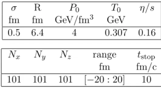
Here, we demonstrate the capability of running 2+1D ideal and viscous Relativistic Hydro-Dynamics (RHD) simulations with ECHO-QGP in the case of fluctuating Glauber-MC initial conditions. The local temperature profile is set at the initial time τ = 1 fm/c for one particular nuclear configuration generated through the Glauber-MC routine implemented in ECHO-QGP (we assume Au-Au collisions with bmax = 20, σ = 0.6 fm,
K = 37.8 GeV/fm2, and α = 0.2); then the subsequent evolution is followed both in the ideal and in the viscous case. In Fig. 2.3 the initial and later stages of the evolution at τ = 5 and 10 fm/c are shown, where the upper row refers to the ideal run and the lower one to the viscous run. Here we assume a square numerical box ranging from −15 to 15 fm and made up by 151 grid points in both directions. The equation of state applied here is the one computed by ref. [102] (see next subsection), while in the viscous run we set η/s = 0.08.
Clearly, the dynamical effects of shear viscosity are reflected in the smoother spatial profiles: the surfaces of discontinuity arising from the transverse expansion of the initial peaks of energy (shock fronts) are clearly
ECHO-QGP 0 100 200 300 400 Npart 0.0001 0.001 0.01 1/N ev (dN ev /dN part ) Glauber-MC Au-Au @ 200 GeV σ NN=42 mb 0 500 1000 1500 N coll 1e-06 1e-05 0.0001 0.001 0.01 1/N ev (dN ev /dN coll ) Glauber-MC Au-Au @ 200 GeV σ NN=42 mb
Figure 2.2: The participant and binary-collision distribution from the
Glauber-MC simulations of Au-Au events at√sN N= 200
Figure 2.3: Temperature scans at various times – at τ = 1, 5, and 10 fm/c – obtained from inviscid (upper panel) and viscous (lower panel) ECHO-QGP simulations with Glauber-MC initial conditions. The differences between the two cases are clearly visible. The effect of shear viscosity can be seen in the smoothening of the profiles.
visible only in the inviscid case. These results demonstrate the capability of ECHO-QGP to handle also complex initial conditions with events displaying sizable fluctuations. The full analysis including the study of higher-order flow harmonics, of the impact on the freeze-out stage and of the final particle spectra is beyond the scope of the present investigation and is left for future work.
2.2
Equation of State
Solving hydrodynamics equations requires the knowledge of the Equation of State (EoS) of the system. Although the code is already designed to handle any form of P = P(e, n), in the present work we just consider the case P = P(e), i.e. the case of a barotropic fluid. ECHO-QGP allows the use of any tabulated EoS of this kind, if provided by the user in the format (T, e/T4, P/T4, c2s), with c2s≡ dP/de, the square of the speed of sound.
However, some choices are already implemented in the code and are of-fered to the user. Test runs can be performed with the ideal ultrarelativistic
ECHO-QGP
EoS P = e/3. More precisely, we set in these cases
P = e/3 = gπ 2 90 T 4, c2 s= 1 3,
where g = 37 for a non-interacting QGP with 3 light flavors.
More realistic QCD EoS’s are included in the package, in the tabulated form mentioned above, and can be selected by the user such as the EoS of ref. [102], arising from a weak-coupling QCD calculation with realistic quark masses and employed in the code by Romatschke [35].
ECHO-QGP includes also two tabulated EoS’s obtained by matching a Hadron-Resonance-Gas EoS (HRG EoS) at low temperature with the continuum-extrapolated lattice-QCD results by the Budapest-Wuppertal collaboration [103]. The HRG EoS was obtained by summing the con-tributions of all hadrons and resonances in the PDG up to a mass of 2 GeV: P =
rPr. In the classical limit T ≪ mr (quantum corrections are
included for pions, kaons and η’s) one has simply, for the pressure of the resonance r: Pr= gr T2m2r 2π2 e µr/TK 2 mr T , (2.7)
and the density of resonance r in the cocktail is given by
nr ≡ ∂P ∂µr T = gr T m2 r 2π2 e µr/TK 2 mr T . (2.8)
In the Chemical Equilibrium case (CE) in the hadronic phase all the chemical potentials vanish ({µr= 0}) and the multiplicity of any resonance
r is simply determined by the temperature through the ratio mr/T . On
the other hand experimental data provide evidence that the chemical freeze-out – in which particle ratios are fixed – occurs earlier than the kinetic one, in which particle spectra gets frozen. A realistic EoS should in principle contain the correct chemical composition in the hadronic phase. This can be enforced in the following way. At the chemical freeze-out temperature Tc the abundances nr of all the resonances are determined by
Eq. (2.8) with µr= 0. Afterwards, the fireball evolves maintaining Partial
Chemical Equilibrium (PCE): elastic interactions mediated by resonances (ππ → ρ → ππ, Kπ → K∗ → Kπ, pπ → ∆ → pπ...) are allowed, changing the abundance of the single resonances r, but conserving the “effective
0 0.05 0.1 0.15 0.2 0.25 0.3 0.35 0.4 T (GeV) 0 1 2 3 4 5 P/T 4
Full Chemical Equilibrium PCE from T=0.170 GeV PCE from T=0.165 GeV PCE from T=0.160 GeV PCE from T=0.155 GeV PCE from T=0.150 GeV lattice-QCD 0 0.2 0.4 0.6 0.8 1 ε (GeV/fm3) 0 0.05 0.1 0.15 0.2 P (GeV/fm 3) HRG+LAT, CE HRG+LAT, PCE Matching HRG-lQCD @ T=150 MeV
Figure 2.4: Upper panel: HRG EoS, with chemical (CE, black con-tinuous line) and partial chemical equilibrium (PCE, col-ored dotted/dashed lines), vs the lattice-QCD results of Ref. [103] (turquoise points). Lower panel: the EoS P (e) resulting from the matching of HRG with lattice-QCD results, in the CE (in black) and PCE (in red) cases. The matching has been performed at the temperature T = 150 MeV.