i
To Alessandra, Mamma, Pap`a, Milena e Nonna
Available energy is the main object at stake in the struggle for existence and the evolution of the world. Ludwig Eduard Boltzmann
Acknowledgements
Firstly, I would like to express my sincere gratitude to my supervisor Dr. Fabio Lepreti for the continuous support of my PhD study and related re-search. His guidance helped me in all the time of research and writing of this thesis.
Besides my supervisor, my sincere thanks also goes to Prof. Vincenzo Carbone for his motivation and immense knowledge, I was honored to work with him.
My deepest heartfelt appreciation goes to Dr. Antonio Vecchio for his insightful suggestions, constructive comments and warm encouragement.
I would like to show my greatest appreciation to Dr. Giuseppe Consolini and Dr. Monica Laurenza for their support to my research, their invaluable encouragement and suggestions. Without they precious support it would not be possible to conduct some part of my research.
Acknowledgements need to be due to Dr. Mirko Piersanti and Prof. Um-berto Villante for their kindness and courtesy, in addition to their support in my research.
A remarkable thanks also goes to Dr. Paola De Michelis for her courtesy and knowledge, very useful in several parts of my research.
Finally, I want to thank my extra-european co-author, Dr. E.W. Cliver, for his patience and kindness as well as his knowledge, always useful during my research activity.
A special thanks to my family. Words cannot express how grateful I am to my mother, my father, my sister and my grandmother for all of the sacrifices that you’ve made on my behalf.
I would also like to thank Dr. Christian Leonardo Vasconez Vega for his sincere and honest friendship, I wish him all the best for his life.
At the end I would like express appreciation to my beloved girlfriend Alessandra who was always my support in the moments when there was no one to answer my queries, whose enthusiasm, interest and support have given me the motivation to realize this achievement.
Sommario
Lo studio delle relazioni Sole–Terra riguarda l’analisi e comprensione dei fenomeni di origine solare che provocano effetti sull’ambiente circum-terrestre. Il Sole `e la sorgente primaria di energia sulla Terra ed `e proprio l’energia che continuamente riceviamo dal Sole che consente, all’interno di un sistema complesso noto come sistema climatico, di poter raggiungere temperature medie superficiali che consentono lo sviluppo della vita sul nos-tro pianeta, anche se con differenze da luogo a luogo e da stagione a sta-gione. Inoltre, l’estrema complessit`a e variabili`a delle condisioni fisiche del Sole determina cambiamenti sia globali che locali all’interno dell’eliosfera. In particolare, questi cambiamenti sono legati a fenomeni di attivit`a mag-netica che avvengono sia all’interno del Sole che nella sua atmosfera, che si manifestano attraverso variazioni dell’irradianza solare (dall’ultravioletto fino ai raggi X), emissioni di massa coronale e brillamenti solari (flares), che sono caratterizzati dal rilascio di grandi quantit`a di energia e particelle ad alta velocit`a. Quest’ultime, con una velocit`a media di circa 450 km/s ed una temperatura che raggiunge il milione di gradi, formano il “vento so-lare”, che interagisce con la nostra magnetosfera esercitando su di essa una pressione tale da determinarne cos`ı la forma, ma anche i suoi cambiamenti. Entro circa otto minuti dalla comparsa del fenomeno sul Sole, l’ambiente circumterrestre viene raggiunto dall’ondata di radiazione ultravioletta ed X che viaggia alla velocit`a della luce nel vuoto, producendo una fortissima ionizzazione dell’alta atmosfera, con fortissimi disturbi nelle radiocomuni-cazioni. Circa un’ora dopo, giungono i protoni pi`u veloci, appena deviati dal campo magnetico terrestre. Nelle successive 20–40 ore, la maggior parte delle particelle, che per effetto della deflessione generata dal campo mag-netico terrestre si concentrano nelle regioni polari, penetra all’interno della magnetosfera, generando perturbazioni alle correnti presenti e producendo una intensa ionizzazione della ionosfera. Viene cos`ı generata quella che `e nota come tempesta geomagnetica che innesca diversi effetti: dal malfun-zionamento delle radio– e tele–comunicazioni allo sfasamento delle bussole, fino a disturbi nella comunicazione GPS e a danni all’elettronica dei satel-liti, cos`ı come possibili serie conseguenze sulla salute degli astronauti in orbita. Nel cielo notturno delle regioni polari si sviluppa una forte lumi-nescenza caratteristica, nota come aurora polare, attraverso cui il cielo
vi
pare drappeggiato da coltri luminescenti che ondeggiano, intensificandosi ed attenuandosi per diverse ore. Al di l`a di queste evidenti manifestazioni, non vi `e alcun dubbio sul fatto che il ciclo di attivit`a solare, un fenomeno quasi– periodico in cui si alternano, su un periodo di circa 11 anni, fasi di massima e minima attivit`a solare, produca effetti sulla Terra, sulle sue vicende me-teorologiche, sulle stagioni, forse sulla fisiologia stessa delle piante e degli animali, uomo compreso.
Lo scopo di questo lavoro di tesi riguarda lo studio, l’analisi e la model-lizzazione dei fenomeni che avvengono nell’ambiente circumterrestre, dalla magnetosfera fino alla superficie terrestre, passando per la ionosfera, nonch`e l’evoluzione e la dinamica del clima terrestre, in relazione alle variazioni dell’attivit`a solare.
In particolare, viene affrontato lo studio delle interazioni tra il vento so-lare e la magnetosfera terrestre nel corso di due tempeste geomagnetiche, avvenute nello stesso giorno, il 17 marzo, ma in due anni differenti, 2013 e 2015, e note come tempeste di San Patrizio. In tale studio, si identificano le scale caratteristiche di oscillazione presenti sia in dati relativi al vento solare (campo magnetico e tasso di trasferimento di energia) che alla dinamica delle correnti aurorali ed equatoriali (auroral electrojets e ring current), mediante l’utilizzo di una tecnica avanzata di decomposizione di segnali nota come Empirical Mode Decomposition (EMD). Da un’analisi di correlazione sia lineare che non lineare, basata sulla teoria dell’informazione (Delayed Mu-tual Information, DMI), `e possibile verificare quantitativamente l’esistenza di una separazione di scala tra processi legati alla dinamica interna della magnetosfera (e quindi non direttamente guidati dalle fluttuazioni del vento solare) e processi in cui il vento solare induce variazioni alla stabilit`a della configurazione magnetosferica. Questi processi vengono identificati come “loading–unloading mechanism” e “directly driven process”. Il primo `e legato alla dinamica interna della magnetosfera ed in particolare agli effetti convettivi delle correnti di coda sulle altre correnti magnetosferiche, men-tre il secondo alle variazioni della struttura della magnetosfera direttamente connesse con i cambiamenti osservati nelle condizioni del vento solare.
Grazie allo studio combinato di misure del campo geomagnetico, ottenute mediante l’utilizzo di magnetometri terrestri, e di misure del campo magne-tosferico, ottenute grazie all’ausilio dei satelliti geostazionari della missione GOES, `e stato possibile evidenziare il contributo della ionosfera alle vari-azioni del campo magnetico terrestre sia durante periodi di quiete del vento solare che in periodi in cui si osservavano tempeste geomagnetiche. Inoltre, `e stato possibile identificare il contributo a grande scala del campo geomag-netico che potrebbe essere utilizzato ai fini della definizione di un nuovo indice locale di attivit`a geomagnetica per monitorare le variazioni sia nei giorni di quiete che in un periodo di disturbo.
Nell’ambito dei fenomeni a scale temporali pi`u brevi, `e stata, poi, pro-posta una validazione di un modello di previsione di particelle energetiche su
vii un periodo diverso rispetto a quello su cui era stato validato in precedenza. I parametri di valutazione, ovvero la probabilit`a che un evento sia previsto e si verifichi cos`ı come il tasso di falsi allarmi, risultano in accordo con i val-ori precedentemente trovati, dimostrando la robustezza e l’accuratezza del modello di previsione. Inoltre, attraverso lo studio dei parametri utili alla validazione del modello stesso (localizzazione sulla superficie solare, emis-sione di raggi X e onde radio) `e stato possibile evidenziare le differenze nell’attivit`a solare degli ultimi due cicli solari (ciclo 23 e 24). In particolare, si `e notata una sensibile riduzione nel numero di fenomeni di attivit`a so-lare noti come brillamenti solari (fso-lares) di circa il 40% con una conseguente diminuzione degli eventi connessi alla generazione di particelle energetiche nell’ambiente circumterrestre.
Per quel che riguarda invece la dinamica a grande scala delle relazioni Sole–Terra sono state studiate prevalentemente le variazioni a grande scala osservate nel corso della storia paleoclimatica del clima terrestre e due mod-elli di bilancio energetico al fine di descrivere i cambiamenti climatici cos`ı come le condizioni per l’abitabilit`a della Terra.
In particolare, dall’analisi delle concentrazioni dell’isotopo 18 dell’ossigeno, nei carotaggi eseguiti al polo Nord ed al polo Sud e riferiti all’ultimo pe-riodo glaciale, 20.000–120.000 anni fa, `e stato possibile individuare due cicli di variabilit`a all’interno delle variazioni del clima terrestre: una di-namica su scale temporali dell’ordine di 1.500 anni, caratterizzata da ra-pidi e repentini incrementi di temperatura noti come eventi di Dansgaard– Oeschger, e l’evoluzione, su scale tipiche di decine di migliaia di anni, asso-ciata all’alternarsi di periodi globalmente pi`u caldi o pi`u freddi. Mentre gli eventi di Dansgaard–Oeschger sono associati a fluttuazioni di temperatura all’interno di uno stesso stato climatico, la dinamica a grande scala tem-porale `e legata a fluttuazioni che avvengono tra due diversi stati climatici, caratterizzati da diverse temperature globali, ed identificabili come fasi sta-diali e interstasta-diali nel corso di un periodo glaciale. Inoltre, `e stato osservato come i cambiamenti climatici che avvengono al polo Nord siano guidati da precedenti variazioni nella storia climatica terrestre registrati nell’emisfero opposto, con un ritardo temporale dell’ordine di 3.000 anni che potrebbe essere legato a fenomeni connessi con la circolazione termoalina oceanica.
Infine, all’interno del contesto dei modelli climatici basati sull’equilibrio termico tra la radiazione solare incidente e quella emessa dalla superficie ter-restre, `e stato sviluppato un modello che consente di descrivere l’evoluzione della temperatura sulla superficie terrestre al variare della latitudine, dell’irradianza solare e dell’effetto serra. In particolare, i risultati delle simulazioni nu-meriche mostrano come l’effetto serra sia di fondamentale importanza all’interno dei meccanismi di stabilizzazione e regolazione del clima terrestre cos`ı come i cambiamenti ciclici e non, osservati nell’irradianza solare, possono influen-zare l’evoluzione della temperatura terrestre. In particolare, in riferimento alle attuali condizioni di irradianza solare `e stato osservato un
compor-viii
tamento oscillante legato alle fluttuazioni di temperatura, con variazioni dell’ordine di ∼ 3 ◦C ed un periodo dell’ordine di circa 800 anni, che potrebbe essere utile per descrivere il comportamento quasi–periodico ev-idenziato dall’analisi di serie temporali legate alle variazioni climatiche.
Abstract
The large variability of the physical conditions of the Sun, over a wide range of spatial and temporal scales, represents the primary source which determines global and local changes inside the heliosphere and, what is per-haps more interesting, in the near Earth space. However, due to the extreme complexity of the system, nonlinear interactions among different parts of the Sun–Earth system play a key role, enormously increasing the range of phys-ical processes involved. Indeed, fluctuations in the magnetic field within the solar atmosphere act as a complex modulation of plasma conditions in the interplanetary space, producing sudden enhancements of the solar energetic particles (SEP) fluxes and cosmic rays, as well as sudden coronal mass ejections (CMEs), or solar irradiance changes in several spectral ranges (from UV to visible). These events are associated with the origin of geo-magnetic storms, which have important effects on our technological society, and possibly on global changes in the climate conditions through complex interactions with the Earth’s atmosphere. The investigation of the physical processes which mainly affect solar and interplanetary space conditions, and the observation and understanding of the interactions of the solar wind with the Earth’s magnetosphere are crucial to be able to predict and mitigate those phenomena that affect space and ground infrastructures or impair the human health.
This thesis addresses, through both data analysis and theoretical models, some of the main issues concerning the nature of the variability of solar activity which affect Space Weather and Earth’s climate.
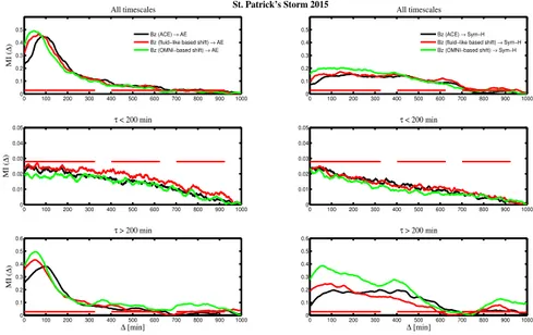
The solar wind–magnetosphere coupling during geomagnetic storms is investigated considering the two events occurred on March 17, 2013 and the same day of 2015, well–known as St. Patrick’s Day storms. To this pur-pose, we analyze interplanetary magnetic field and energy transfer function (i.e., known as Perreault–Akasofu coupling function) time series to study the solar wind variability, as well as geomagnetic indices, related to the ring current and auroral electrojets activity, to investigate their response to so-lar wind variations. Through the Empirical Mode Decomposition (EMD) we identify the intrinsic oscillation timescales in both solar and magneto-spheric time series. A clear timescale separation between directly driven processes, through which solar wind affects magnetospheric current systems,
x
and loading–unloading processes, which, although triggered by solar wind variations, are related to the internal dynamics of the magnetosphere, is found. These results are obtained by the combined analysis between EMD and information theory (i.e., Delayed Mutual Information analysis) allowing us to investigate linear and non–linear coupling mechanisms, without any assumptions on the linearity or stationarity of the processes.
By using both geostationary and ground–based observations of the Earth’s magnetic field, we investigate, then, the role of the ionosphere into the varia-tions of the geomagnetic field, during both quiet and disturbed periods. We also provide a separation of both magnetospheric and ionospheric signatures in the geomagnetic field as well as the large–timescale contribution which could be useful to define a new local index to monitor geomagnetic activity, since it is free from any magnetospheric or ionospheric contribution.
In the framework of the short–term effects of solar activity on Earth’s environment, we investigate the occurrence of SEP events in both solar cycles 23 and 24 and we validate a short–term prediction model (termed ESPERTA) on a new database, different from that on which it was previ-ously evaluated. We found a reduction of SEP events occurrence of ∼40%, suggesting that several differences can be found between the latter two solar cycles. Although these differences, the performance of the ESPERTA model are quite similar in both periods, confirming the robustness and efficiency of the model.
Concering solar–terrestrial relations on larger timescales we propose two different climate models to investigate the role of solar irradiance changes on the stability of the Earth climate as well as the effects of greenhouse vari-ations on the planetary surface temperature. We find that the greenhouse effect plays a key role into the stabilization and self–regulation properties of the Earth climate and that solar irradiance changes could affect the evo-lution of Earth’s climate. Interestingly, for the present conditions of solar irradiance an oscillatory behavior is found with temperature fluctuations ∆T ∼ 3 K and oscillations on 800–yr timescale that needs to be investi-gated with more accuracy because it can reproduce several quasi–periodic behaviors observed in climatic time series.
Moreover, by analyzing the time–behavior of oxygen isotope δ18O dur-ing the last glacial period (i.e., 20–120 kyr before present) we find that the climate variability is governed by physical mechanisms operating at two different timescales: on 1.500–yr timescale, climate dynamics is related to the occurrence of fast warming events, known as Dansgaard–Oeschger (DO) events, while on multi–millennial timescales, climate variations are related to the switch between warming/cooling periods. While DO events can be seen as fluctuations within the same climate state, warming/cooling phases are associated to fluctuations between two climate states, charac-terized by global increase/decrease of temperature. Finally, the results of cross–correlation analysis show that Antarctic climate changes lead those
xi observed in Northern Hemisphere with a time delay of ∼3 kyr, which could be related to the oceanic thermohaline circulation.
Contents
1 Introduction 1
2 The Hilbert-Huang Transform (HHT) 11
2.1 The Empirical Mode Decomposition (EMD) . . . 11
2.2 Hilbert Spectral Analysis . . . 13
I Short-term solar-terrestrial processes 17 3 Solar wind and Earth’s magnetosphere 19 3.1 The solar wind . . . 19
3.2 The Earth’s magnetosphere . . . 21
3.2.1 Magnetospheric Currents . . . 22
3.2.2 Geomagnetic storms and substorms . . . 28
3.2.3 Geomagnetic indices . . . 29
4 St. Patrick’s Day storms in 2013 and 2015 35 4.1 Introduction. . . 36
4.2 Methodology . . . 37
4.2.1 Geospace Conditions . . . 37
4.2.2 Data sets . . . 37
4.2.3 The Empirical Mode Decomposition (EMD) Method . 39 4.2.4 The Delayed Mutual Information (DMI) Approach . . 41
4.3 Results and Discussion . . . 43
4.4 Effect of propagation from L1 position to bow shock nose . . 47
4.4.1 OMNI-based propagation method . . . 48
4.4.2 Fluid-like based propagation method . . . 50
4.4.3 Effect on DMI analysis. . . 51
4.5 Summary and Conclusions . . . 52
5 Magnetosphere-Ionosphere coupling 57 5.1 Introduction. . . 57
5.2 Data sets and methodology . . . 58 xiii
xiv CONTENTS
5.2.1 Empirical Mode Decomposition (EMD) and
Standard-ized Mean Test (SMT) . . . 59
5.3 Magnetospheric and ground observations: EMD approach . . 60
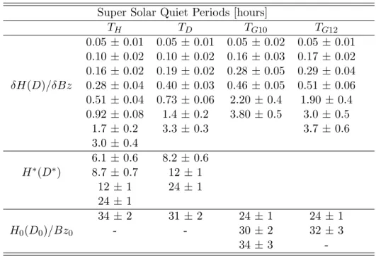
5.3.1 Super Solar Quiet (SSQ) period: 10-12 October 2003 . 60 5.3.2 Storm Time (ST) event: 28 October-01 November 2003 64 5.4 Results and Discussion . . . 67
5.4.1 SSQ contributions . . . 67 5.4.2 ST contributions . . . 69 5.5 Summary . . . 70 5.5.1 Magnetosphere . . . 70 5.5.2 Ground . . . 71 5.6 Conclusions . . . 72
6 Short-term forecast of SEP events 77 6.1 Introduction. . . 77
6.2 Database . . . 79
6.2.1 Time-Integrated SXR Intensity . . . 81
6.2.2 Time-Integrated 1 MHz Radio Intensity . . . 83
6.3 X-ray and Type III bursts statistics . . . 84
6.3.1 Comparison of Numbers and Sizes of Events During the Rise Phases of Cycles 23 (Sep 1996 - Sep 2002) and 24 ( Dec 2008 - Dec 2014) . . . 84
6.3.2 Comparison of Numbers and Sizes of Events During 1995-2005 and 2006-2014 . . . 86
6.3.3 Comparison of Probability Density Functions for 1995-2005 and 2006-2014 . . . 87
6.3.4 Solar Longitude Distribution of ≥ M2 SXR Flares With and Without Associated SEP Events for 1995-2005 and 2006-2014 . . . 89
6.4 Validation of ESPERTA . . . 90
6.5 Evaluation of SEP event warning times . . . 93
6.6 Discussion and conclusions. . . 93
II Long-term solar-terrestrial processes 99 7 Solar irradiance and climate 101 7.0.1 Solar irradiance variations at different timescales . . . 102
7.1 The Earth’s climate system . . . 103
7.1.1 Solar influence on climate . . . 105
7.1.2 The greenhouse effect . . . 107
CONTENTS xv
8 Temperature changes during an ice-age 109
8.1 Introduction. . . 109
8.2 Data sets . . . 111
8.3 EMD results . . . 112
8.4 Potential analysis . . . 115
8.5 The north-south asynchrony . . . 118
8.6 Conclusions and discussion . . . 119
9 A modified Daisyworld model 123 9.1 Introduction. . . 123
9.2 The model. . . 124
9.3 Stability analysis . . . 126
9.3.1 No greenhouse effect (g(T ) = 1) and no diffusion (κ(θ) = 0) . . . 127
9.3.2 Greenhouse effect (g(T ) 6= 1) and no diffusion (κ(θ) = 0)127 9.3.3 Greenhouse effect (g(T ) 6= 1) and constant diffusion (κ(θ) = constant) . . . 129
9.4 Numerical results . . . 130
9.4.1 The effects of a non-uniform heat diffusion . . . 132
9.4.2 The greenhouse effect . . . 134
9.4.3 Dependence on initial conditions . . . 135
9.4.4 Multiple steady-states . . . 136
9.5 Conclusions . . . 138
10 On the stability of a climate model 143 10.1 Introduction . . . 143
10.2 The model . . . 145
10.3 Multiple steady–states . . . 147
10.3.1 Steady–states in absence of vegetation . . . 147
10.3.2 Steady–states in presence of vegetation . . . 149
10.4 Stability analysis of climate states . . . 151
10.4.1 Stability of the climatic states in absence of vegetation 151 10.4.2 Stability of the vegetated steady–state solution . . . . 152
10.5 Conclusions . . . 154
11 Summary & Conclusions 161
Appendix A Abbreviations 165
Appendix B Physical Constants 167
Appendix C Kernel Density Estimator 169
Chapter 1
Introduction
The Solar-Terrestrial interactions involve physical processes related to the coupling between the Sun’s variability and the Earth’s environment, includ-ing both dynamical and energetic processes. These phenomena take place in the Heliosphere, a large bubble formed by the hot plasma blowing out from the Sun (i.e., the solar wind), in which the Sun and planets reside. The solar wind creates and maintains this bubble against the outside pressure of the interstellar medium, formed by hydrogen and helium gases permeating the Milky Way Galaxy. The solar wind flows outward from the Sun until encountering the termination shock, where motion slows abruptly, passing through the shock and entering the heliosheath, a transitional region which is in turn bounded by the outermost edge of the heliosphere, called the heliopause. The investigation of these phenomena is made in the frame-work of Heliophysics, the science of the Sun–solar-system connections, ex-ploration, discovery and understanding of our space environment. It focuses on the Sun and its effects on Earth, the other planets of the solar system, and the changing conditions in space. Heliophysics studies the magneto-sphere, ionomagneto-sphere, thermomagneto-sphere, mesosphere and upper atmosphere of the Earth and other planets, combined with the science of the Sun, corona, he-liosphere and geospace environment. It encompasses particle acceleration mechanisms, space weather and radiation hazards, solar activity and cycles, planetary climate, space plasmas and changes in magnetic field topology (NASA,2006).
Nowadays, the increase in knowledge of the Sun’s magnetic activity changes allows the investigation of several phenomena occurring in the Earth’s environment, covering a wide range of temporal and spatial scales, among which the interaction between the solar wind and the Earth’s magnetic field (geodynamo field) and the effects on the atmospheric and climate systems. The solar wind alters the magnetospheric configuration, modifying the mag-netospheric current systems through the injection of charged particles, and affects the ionospheric layers (i.e., F and E layers). Conversely, changes
2 CHAPTER 1. INTRODUCTION
Figure 1.1: The structure of the Heliosphere.
in solar irradiance can affect the atmospheric circulation and composition (i.e., greenhouse effect), and the ocean-atmosphere coupling, producing lo-cal micro-climates and modifying the thermal equilibrium between incoming and outcoming energy fluxes.
One of the main aims in heliospheric studies corcerns the effects of mag-netic fields on ionized matter. Indeed, this field-plasma coupling character-izes many different phenomena, ranging from the Earth’s ionosphere to the Sun’s surface, such as the acceleration of ions and electrons to higher ener-gies (with respect to the plasma bulk kinetic energy) through wave-particle interaction. This characterizes large solar flares and their associated coronal mass ejections, producing changes of the magnetic field topology, and conse-quent effects on the Earth’s environment when they interact with the Earth’s magnetic field (i.e., generation of geomagnetic storms and substorms, au-rora manifestation, Van Allen radiation belts enhancements). The coupling with neutral components within the plasma also produces several effects in terms of electrical conductivity changes, shifting the ionization balance by collisions and modifying the ionospheric and upper atmospheric electrody-namics (i.e., affecting the Pedersen and Hall conductivities, radiative trasfer and stratospheric ozone dynamics). Moreover, solar photons are Earth’s primary energy source: Earth is habitable only because the Sun shines, ra-diating energy throughout the heliosphere, and the greenhouse effect controls the thermal energy balance, giving rise to a mean global surface tempera-ture T ∼ 10 − 15◦C (without greenhouse effect it would be ∼ −20◦C). The Sun shines because its surface, warmed by energy produced in its nuclear burning core, is hotter (∼ 5770 K) than the surrouding cosmos (∼ 4 K). Electromagnetic energy traveling radially outward from the Sun reaches the Earth’s upper atmosphere, it is continously absorbed and re-emitted within the atmosphere until it reaches the Earth’s surface. The average total so-lar irradiance, at a distance of 1 astronomical unit (AU), is 1361 ± 4 W m−2, with higher energy confined in the visible part of the spectrum (due
3 to solar surface temperature value); conversely, Earth emits in the infrared part of the spectrum (following the Wien’s displacement law). The thermal energy balance between solar incoming radiation and that outgoing from Earth’s surface determines the conditions for life (habitability), the climate evolution and affects the cryosphere-atmosphere-biosphere interactions.
The Sun is a magnetically variable star which produces profound con-sequences and impacts on planets with intrinsic magnetic field, with at-mospheres or with both properties (like Earth). Its magnetic activity and the associated changes evolve on timescales that range from minutes up to billions of years, involving nonstationary and nonequilibrium active pro-cesses, broadly regarded as solar activity. Whereas this concept is quite common nowadays, it is neither straightforwardly interpreted nor unam-biguously defined (Usoskin,2013). For instance, magnetic variability on the solar surface, eruption phenomena, coronal activity, interplanetary transient phenomena (i.e., corotating interaction regions, interplanetary coronal mass ejections), solar energetic particles as well as geomagnetic storms and sub-storms, tail current disruption, wave-particle interactions can be related to the concept of solar activity (Parker,1965;Gonzalez et al.,1994;Cane and
Lario, 2006; Love, 2011). Several indices, quantifying solar activity, have
been proposed to represent different observables and caused effects, for both solar and geospace monitoring. Most of these indices are well-correlated to each other, due to the dominant 11-year Schwabe solar cycle (Schwabe,
1843), but they differ in short-term and/or long-term dynamics. The most common used indices of solar activity are reported in Table1.1.
Indices Type Associated physical meaning
Wolf Sunspot Number (WSN) Solar Magnetic spots
Group Sunspot Number (GSN) Solar Active regions
Flare index Solar Solar flares activity
F10.7 index Solar Radio-flux at λ = 10.7 cm
MgII / Ca II-K Solar Spectral emission properties Sym-H / Dst Geomagnetic Magnetospheric ring current activity AE, AU, AL, AO indices Geomagnetic Auroral electrojets activity
Table 1.1: Solar and geomagnetic indices used to monitor solar activity. The short-term (from minutes to months) variability of the solar ac-tivity is generally associated with eruptive phenomena (i.e., faculae, flares, coronal mass ejections) which extend from the solar surface to the inner he-liosphere, carried out from the Sun by the solar wind (Emery et al.,2011). The dominant short-term quasi-periodicity in the solar activity (found in several solar wind parameters like speed and interplanetary magnetic field) is the rotation of the Sun, that is the apparent (synodic) rotation, known as Carrington rotation, with a period of ∼27 days (as seen at the Earth) at ∼25◦ heliolatitude near the solar disk part in which several active regions
4 CHAPTER 1. INTRODUCTION develop. The sidereal rotation rate of the Sun is ∼24 days at the solar equa-tor increasing to ∼30 days at the poles (Chandra et al., 2009). Studies of the periodicities in the near-Earth solar wind and geomagnetic indices have found a 27-day signature, ranging between 25- and 29-day periods (
Sval-gaard and Wilcox, 1975; Emery et al., 2011). Mursula and Zieger (1996)
found a second harmonic structure of the solar rotation periodicity (i.e., a ∼13.5-day period) in solar, heliospheric, and Earth-based parameters. In-deed, the analysis of the power spectra of the sunspot number, the Ca K-line index, the Mg II core to wing (c/w) ratio and Geostationary Operational Environmental Satellites (GOES) background X-ray intensity showed peaks at the fundamental 27-day periodicity and at its second harmonic. The 13.5-day amplitudes in these solar variables indicated the presence of two active solar longitudes approximately 180◦ apart. The position of the active solar longitudes could abruptly change by even 90◦ between two successive 13.5-day activations. Higher (and lower) harmonics were also found (Emery
et al., 2009, 2011), particularly evident during solar minimum conditions
(of the Schwabe cycle), which can be related to high-speed streams (HSSs) solar structures. These are the 7-day and 9-day periodicities which can be associated to a sub-harmonic structure of the synodic solar rotation (∼ 27 days), due to the four-sector structure topology of the solar magnetic field. This structures can also lead to the formation of corotating interaction re-gions (CIRs) (Thayer et al.,2008;Emery et al., 2009). On the other hand, lower harmonics (∼ 40, 54, 81 days) correspond to multiple or combinatory timescales of the 27-day periodicity (Willson and Mordvinov,1999).
The observed quasi-periodicities act in different ways on the Earth’s environment, producing short-term transient phenomena (like geomagnetic storms and substorms), occurring when CMEs hit the Earth’s magneto-sphere, and generating global and local disturbances of the geomagnetic field, also able to modify the ionospheric electrodynamics via the auroral electrojets dynamics. Moreover, daily solar radiation changes also affect ionospheric current systems (i.e., Solar quiet mid-latitude current pattern) and atmospheric composition via ionization processes of the atmospheric gases (i.e., oxygen, ozone, carbon dioxide). Solar rotational structures are also responsible for ultra-low frequency (ULF) waves generation in the mag-netosphere and enhancements of the Van Allen electrons (via wave-particle interaction which produces relativistic electrons energization) (Mann et al.,
2004).
A clear evidence of short-term Sun-Earth connection is the well-known solar storm of 1859, famous as Carrington event (Carrington,1860;Hodgson,
1860), classified as the first recognized space weather event (Cliver and
Sval-gaard,2004). At 11:18 AM of the cloudless morning of Thursday, September
1, 1859, Richard Carrington, widely accepted as one of the England’s fore-most solar astronomers, was observing the central disk portion of the Sun, sketching a group of sunspots (see Figure1.2).
5
Figure 1.2: Richard Carrington (on the left) and the sunspots sketched on Sep 1, 1859 (on the right).
Suddenly, before his eyes, two brilliant enhancements of white light ap-peared over the sunspots, intensified rapidly, and became kidney-shaped. Realizing that he was witnessing something unprecedented and “being some-what flurried by the surprise,” Carrington later wrote, “I hastily ran to call someone to witness the exhibition with me. On returning within 60 seconds, I was mortified to find that it was already much changed and enfeebled”. Just before dawn the next day, skies all over the Earth erupted in red, green, and purple auroras so brilliant that newspapers could be read as easily as in daylight. Indeed, stunning auroras pulsated even at near tropical latitudes over Cuba, the Bahamas, Jamaica, El Salvador, and Hawaii. Even more disconcerting, telegraph systems worldwide went haywire, spark discharges shocked telegraph operators and set the telegraph paper on fire. Even when telegraphers disconnected the batteries powering the lines, aurora-induced electric currents in the wires still allowed messages to be transmitted. What Carrington saw was a white-light solar flare, a magnetic explosion on the Sun, the first one observed from the Earth, while the next day people observed its effect on the Earth’s environment, i.e., large auroral activity (quite far from the Poles) and the first evidence of a geomagnetic storm, causing “technological” disruptions. Now we know that solar flares happen frequently, especially during solar cycle maximum phases, emitting X-rays (recorded by X-ray telescopes in space) and radio noise (recorded by instru-ments in space and on Earth).
In Carrington’s days, however, there were no X-ray satellites or radio telescopes, no one knew the existence of flares, until that September morn-ing when one super-flare produced enough light to reveal the brightness of the Sun itself. Newspapers such as the New York Times were active in run-ning extensive stories about the 1859 solar storm, and collecting reports from other countries. The great geomagnetic storm of 1859 is really composed of two closely spaced massive worldwide auroral events. The first event began on August 28th and the second began on September 2nd. It is the storm on September 2nd that resulted from the Carrington white light flare that occurred on the Sun the previous day. What if a similar biggest solar storm happened today? The explosive heat of a solar flare cannot make it all
6 CHAPTER 1. INTRODUCTION
Figure 1.3: A modern solar flare recorded on Dec 5, 2006, by the X-ray Imager on board of NOAA’s GOES-13 satellite. The flare was so intense that damaged the instrument that took the picture, although researchers believe Carrington’s flare was much more energetic than this one.
the way to our globe, but electromagnetic radiation and energetic particles certainly can. Solar flares can temporarily alter the upper atmosphere, cre-ating, for example, disruptions in signal transmission from a GPS satellite to Earth, causing it to be off. Minutes to hours after a solar flare lights up the sky, a stream of charged particles (electrons and protons) arrive at the Earth, bombarding the magnetosphere. These solar explosions produce bursts of particles and electromagnetic fluctuations into the Earth’s atmosphere, in-ducing electric fluctuations at ground level that could blow out transformers in power grids. Occasionally, a large pulse of charged particles can hit orbit-ing satellites and damage their electronics, while particle radiation is also a big health risk for humans in space. In an increasingly technological world, where almost everyone relies on smartphones, GPS controls not only in-car map system, but also airplane navigation and the extremely accurate clocks that govern financial transactions. These phenomena need to be treated with convergency of several scientific branches, from physics to engineering, to develop a monitoring (and also forecasting) system. The study of these phenomena and their effects on the Earth’s environment and technological impacts is made in the framework of the Space weather. This is a branch of space physics and aeronomy concerned with the time varying conditions on the Sun and in the solar wind, magnetosphere, ionosphere and thermo-sphere that can influence the performance and reliability of space-borne and ground-based technological systems and can endanger human life or health. It is influenced by the solar wind and the interplanetary magnetic field (IMF) carried by the solar wind plasma, inducing a variety of physical phenomena, including geomagnetic storms and substorms, energization of the Van Allen radiation belts, ionospheric disturbances, scintillation of satellite-to-ground radio signals, long-range radar signals, aurora and geomagnetically induced
7 currents at Earth’s surface (Cade and Christina,2015).
However, the main feature of solar activity is its pronounced quasi-periodicity with a period of about 11 years, known as the Schwabe cycle
(Schwabe, 1843). It varies in both amplitude and duration (Usoskin and
Mursula,2003; Vecchio et al., 2017) and it is recognized as a fundamental
feature of solar activity originating from the solar-dynamo process. This 11-year cyclicity is prominent in many other parameters, including solar and geomagnetic indices, but also in climate proxies and observables, as for example Sea Surface Temperature (SST). The background for the Schwabe cycle is the 22-year Hale magnetic polarity cycle (Hale et al., 1919), an observed quasi-periodicity of the sunspot magnetic field polarity reversal due to the inner solar dynamo reversal (Hathaway,2010). Sometimes, the regular time evolution of solar activity is broken up by periods of greatly depressed activity called grand minima, one of the most recent of which was the famous Maunder minimum from 1645-1715 (Eddy,1976,1983). Other grand minima in the past, derived from the analysis of cosmogenic isotope data (Usoskin et al.,2007,2016), include the Sp¨orer minimum around 1450-1550 and the Wolf minimum around the 14th century (Vecchio et al.,2017, Table 3). Although sunspot activity was not completely suppressed and still showed Schwabe cyclicity, sometimes the Dalton minimum (ca. 1790-1820) is also considered to be a grand minimum.
The long-term change in the Schwabe cycle amplitude is known as the secular Gleissberg cycle (Gleissberg,1939, 1948, 1952) with a mean period of about 90 years. However, the Gleissberg cycle is not a cycle in the strict periodic sense but rather a modulation of the cycle envelope with a vary-ing timescale of 60-120 years (e.g.,Gleissberg,1971; Ogurtsov et al., 2002;
Vecchio et al.,2017). Longer (super-secular) cycles cannot be studied using
direct solar observations, but only indicatively by means of indirect proxies such as cosmogenic isotopes and paleo-reconstructions of the solar irradiance and sunspot number (Solanki et al., 2004). These indirect proxies allow to show the existence of several longer cycles, as for example, a cycle with a period of 205-210 years, known as the de Vries or Suess cycle, a prominent feature observed in various cosmogenic data (e.g.,Suess,1980;Usoskin et al.,
2004;Vecchio et al.,2017). Sometimes, variations with a characteristic time
of 600-700 years or 1000-1200 years are discussed (e.g.,Vitinsky et al.,1986;
Steinhilber et al., 2012) but they are intermittent and can hardly be
re-garded as a typical feature of solar activity. A 2000–2400-year cycle is also noticeable in radiocarbon and cosmogenic time series (e.g., Vitinsky et al.,
1986;Usoskin et al.,2016;Vecchio et al.,2017). However, the non-solar
ori-gin of these super-secular cycles (e.g., geomagnetic or climatic variability) cannot be excluded (Usoskin et al.,2016;Vecchio et al.,2017).
How these larger timescale periodicities can affect Earth’s environment? The Sun-Earth connections on large-timescales (above months) are typically related to energy-balance processes, radiative and thermal equilibrium
vari-8 CHAPTER 1. INTRODUCTION ations, atmospheric and climatic effects, principally affecting Earth’s surface temperature evolution. One of the most famous example of Sun-Earth con-nection on large-timescales is the period between 1645 and 1715, known as Maunder minimum (Eddy,1976,1983;Usoskin et al.,2007;Vecchio et al.,
2017). It is also known as the “prolonged sunspot minimum”, since sunspots became exceedingly rare, as noted by solar observers of the time and reported in several works (Sp¨orer,1887, 1889; Maunder,1890,1894). The Maunder minimum is representative of grand minima in solar activity, during which sunspots almost completely vanished on the Sun’s surface and solar wind kept blowing (Cliver et al.,1998;Usoskin, 2013). It was amazingly well re-covered by direct sunspot observations, although they appeared rarely and seemingly sporadically (∼ 2% of the days), without any indication of the Schwabe solar cycle (Usoskin and Mursula,2003). Therefore, some uncer-tainty about its duration is also present: the “formal” duration is 1645-1715 (Eddy,1976), although its deep phase, characterized by apparent absence of solar cycle activity, is often considered as 1645-1700, with a recovery solar cycle variation during 1700-1712 (Usoskin,2013). Usoskin et al. (2001) and
Mursula et al.(2001) have shown that sunspot occurence during the
Maun-der minimum was characterized by two larger sunspot clusters (1652-1662 and 1672-1689), implying a dominant 22-year periodicity in sunspot activity. Interestingly, the Maunder Minimum roughly coincided with the mid-dle part of the Little Ice Age, a period of climatic cooling occurred from ∼ 1300 to ∼ 1800, reaching its chilliest point in the 17th century. Dur-ing the Maunder Minimum, temperature across the Northern Hemisphere declined (if compared to the 20th century averages this decline was about 1 ◦C), contributing to a global crisis that destabilized social life. Indeed, as growing seasons shortened, food shortages spread, economies unraveled, rebellions and revolutions took place. The observed cooling was not the pri-mary cause of these disasters but it often played an important role. Whether there is a causal relationship, however, is still controversial, as no convinc-ing mechanism for the solar activity to produce cold temperatures has been proposed. What seems certain is that many of the coldest decades of the Little Ice Age coincided with periods of reduced solar activity: the Sp¨orer Minimum (1450-1530), the Maunder Minimum (1645-1715), and the Dalton Minimum (1790-1820). However, one of the chilliest periods of all, known as Grindelwald Fluctuation (1560-1630), actually unfolded during a modest rise in solar activity. The current hypothesis for the cause of the Little Ice Age is that it was the result of volcanic action (Miller et al.,2012), which played an important role in bringing about cooler decades, as did the nat-ural internal variability of the climate system. Indeed, both the absence of eruptions and a solar grand maximum likely set the stage for the Me-dieval Climate Anomaly, a warmer period in the Earth’s geological hystory. However, an increase in volcanic eruptions and the associated grand minima states of solar activity can induce lower surface temperature. This occurred
9 in the days of the Maunder minimum when the water in the river Thames and the Danube River froze, the Moscow River was covered by ice every six months, snow lay on some plains all year round and Greenland was covered by glaciers (see Figure1.4).
Figure 1.4: In this 1677 painting by Abraham Hondius, “The Frozen Thames, looking Eastwards towards Old London Bridge”, people are shown enjoying themselves on the ice.
What would happen during a new Maunder Minimum? It is well known that the influence of the Sun on our climate since pre-industrial times, in terms of radiative forcing, is very small compared to the effect of greenhouse gases (IPCC,2014). The estimated increase in radiative forcing due to the Sun since 1750 (just after Maunder Minimum) is only 0.05 W m−2compared to a total increase that is mainly caused by greenhouse gases of 2.29 W m−2.
Bond et al.(2001) showed that a possible larger solar effect on climate could
be related to some amplification mechanisms such as energy stored in oceans and their interaction with atmosphere. Another mechanism is associated to the cosmic rays variations (related to the solar activity) in cloud formation and corresponding changes in atmospheric composition as well as the effect of solar UV changes into the stratospheric ozone dynamics.
If a new grand minimum state occurred this could lead to similar cool-ing of the Earth atmosphere (∼ -0.5◦C) as during the Maunder minimum
(Lockwood et al.,2010), although the current anthropogenic warming would
lead to a temperature increase of ∼ 4◦C, deleting solar activity effects. How-ever, variability in ultraviolet solar irradiance is linked to modulation of the Arctic and North Atlantic Oscillations, suggesting the potential for larger regional surface climate effects. This would induce a wintertime response, producing a cooling over northern Eurasia and eastern United States, simi-lar to the observed temperature reductions during the Little Ice Age (Ineson et al.,2015).
The main purpose of this thesis is the investigation of solar-terrestrial physical processes at different timescales, considering both short- and
long-10 CHAPTER 1. INTRODUCTION term processes, in order to understand the effects of the changing Sun over the Earth’s environment. This thesis includes two main parts: (i) the study of short-term processes characterizing solar activity, and (ii) the investiga-tion of the role of solar irradiance changes on the climate system. Chapter
2 presents the main data analysis technique used to investigate nonlinear and nonstationary time series at different timescales, Chapter 3 illustrates some aspects of the solar wind and Earth’s magnetosphere, while Chapters
4 and 5 focus on solar wind-magnetosphere and magnetosphere-ionosphere couplings, respectively. Then, Chapters 6 presents an empirical model to provide short-term warming of solar energetic particle (SEP) events. Chap-ter 7 describes the main characteristics of the Earth’s climate, Chapter 8
focuses on larger timescales variations of the climate system, while Chapters
9and10present two numerical energy-balance models to investigate climate changes and the role of the greenhouse effect. Finally, a conclusion chapter summarises the current research in the field and highlights possible further areas of research.
Chapter 2
The Hilbert-Huang
Transform (HHT)
Theoretically, data analysis techniques should require no assumptions to be made about the nature of the investigated time series, i.e., neither linearity, nor stationarity should be assumed. This is because the behavior of physi-cal processes that have generated the data is usually not known beforehand. Morever, adaptivity to the analyzed time series would also be a sought after feature, letting the data itself drive the decomposition. The latter criterion ensures both that the extracted components carry physical meaning, and that the influence of mathematical artefacts and assumptions is kept to a minimum (Wu and Huang,2011). Since such a decomposition is only deter-mined by the local characteristic timescales of a time series, its suitability to nonlinear and nonstationary time series analysis is important (Huang et al.,
1998).
In this chapter, the Hilbert-Huang Transform (HHT), an adaptive data analysis technique built with the previous considerations in mind, is pre-sented. It involves two distinct steps, the empirical mode decomposition (EMD) followed by Hilbert spectral analysis.
2.1
The Empirical Mode Decomposition (EMD)
The first step of the HHT is the empirical mode decomposition (EMD), an algorithmic procedure, by which oscillations that present a common lo-cal timeslo-cale are iteratively extracted from the data. The empirilo-cal mode decomposition has been developed to process non-stationary data (Huang
et al.,1998) and successfully applied in many different contexts (Cummings
et al.,2004;McDonald et al.,2007;Terradas et al.,2004;Vecchio et al.,2010;
Wu and Huang,2009), including geophysical systems (Alberti et al., 2014,
2016; Balasis and Egbert, 2006; De Michelis et al., 2012). It is an
adap-tive and a posteriori decomposition method in which the basis functions are 11
12 CHAPTER 2. THE HILBERT-HUANG TRANSFORM (HHT) derived from the data. This technique decomposes a set of observed data X(t) into a finite number m of intrinsic oscillatory functions Cj(t), named
Intrinsic Mode Functions (IMFs), so that X(t) =
m
X
j=1
Cj(t) + r(t), (2.1)
where r(t) is the final residue of the decomposition from which no more IMFs can be extracted. Each mode Cj(t) can be derived by the so-called
sifting process which represents the core of the decomposition procedure. This procedure can be summarized by the following steps:
1. identification of the local extrema of the time series X(t)
2. interpolation of local minima (maxima) by using a spline function to obtain the local envelope emin(t) (emax(t))
3. computation of the mean envelope m1(t) = mean([emin(t), emax(t)])
4. evaluation of the first “candidate” IMF h1(t) = X(t) − m1(t)
The previous steps are iterated k times until the obtained detail h1k =
h1(k−1) − m1k can be identified as an IMF such that the two following
properties are satisfied:
1. the number of extrema and the number of zero-crossings must either be equal or differ at most by one
2. at any point (locally), the mean value of the envelope defined by the local maxima and by the local minima is zero.
In addition, the number of sifting steps to produce an IMF is defined by the stopping criterion proposed by Huang et al. (1998), similar to the Cauchy convergence test, which defines a sum of the difference (standard deviation), σk, between two sifting steps as
σk= T X t=0 |hk−1(t) − hk(t)|2 h2 k−1(t) (2.2)
The sifting process stops when σk is smaller than a given value, typically
into the range 0.2-0.3 (Huang et al., 1998). This is not the only stopping criterion proposed, since there are several works in which different methods have been proposed. One of these is the threshold method proposed by
Flandrin et al.(2004) which sets two threshold values to guarantee globally
small fluctuations and, in the mean while, takes into account locally large excursions. Another one is called the “S Number Criterion”, based on the
2.2. HILBERT SPECTRAL ANALYSIS 13 so-called S-number, which is defined as the number of consecutive siftings for which the number of zero-crossings and extrema are equal or at most dif-fering by one. Specifically, an S-number is pre-selected. The sifting process will stop only if, for S consecutive siftings, the numbers of zero-crossings and extrema stay the same and are equal or at most differ by one.
2.2
Hilbert Spectral Analysis
Once the empirical mode decomposition is completed, the second and last step of the HHT consists in the Hilbert spectral analysis of the previously obtained IMFs. Each IMF and its Hilbert transform are used to construct a complex analytic signal, described by an amplitude modulation - frequency modulation (AM-FM) model. This decomposition into two time-varying parts corresponding respectively to instantaneous amplitude and instanta-neous frequency enables the identification, in a time-varying sense, of how much power (i.e., the square of amplitude) occurs at which time-scale (i.e., the inverse of frequency).
An IMF is an oscillating function modulated in both amplitude and fre-quency, as Cj(t) = Aj(t) cos[Φj(t)], where Φj(t) is the instantaneous phase
of the j-th mode, related to the instantaneous frequency ωj(t) = dΦj(t)/dt
(Huang et al., 1998). Since other decomposition techniques do not
con-sider a time-dependent frequency (e.g. Fourier analysis), this concept of instantaneous frequency is the major point of the EMD technique, allowing a decomposition of non-stationary time series without any assumption on the basis of the decomposition. It can be derived by using the so-called Hilbert-Huang transform (Huang et al.,1998), through which for each Cj(t)
we can derive the corresponding Hilbert transform ˜Cj(t) as
˜ Cj(t) = 1 πP Z +∞ −∞ Cj(t0) t − t0 dt 0 (2.3)
where P denotes the Cauchy’s principal value. The function defined by Eq. (2.3) exists for all Lp space functions, allowing us to define an analytical
signal Z(t) from the conjugate pair (Cj(t), ˜Cj(t)), such that
Zj(t) = Cj(t) + i ˜Cj(t) = Aj(t)eiΦj(t) (2.4)
in which Aj(t) and Φj(t) are the instantaneous amplitude and phase of the
j-th mode, respectively, derived as Aj(t) = q Cj(t)2+ ˜Cj(t)2 (2.5) Φj(t) = arctan ˜ Cj(t) Cj(t) (2.6)
14 CHAPTER 2. THE HILBERT-HUANG TRANSFORM (HHT) In this way, the instantaneous frequency can be derived by the instantaneous phase as ωj(t) = dΦj(t)/dt (Huang et al., 1998). Consequently, a typical
average period Tj can be estimated for all the IMFs as Tj = 2π/ < ωj(t) >t
(<>t representing the time average). The decomposition is clearly local
and complete, which means that the IMFs can reconstruct the original sig-nal (see Eq. (2.1)), while the orthogonality property is not theoretically ensured. However, it can be verified by evaluating the orthogonal index (OI) as proposed in Huang et al. (1998) by checking the inner product of each IMF with respect to the others. In this case, the EMD can be used as a filter through partial sums of a subset of modes (Alberti et al.,2014). Finally, based on numerical experiments on white noise using the empiri-cal mode decomposition (EMD) method,Wu and Huang(2004) empirically found that the EMD is effectively a dyadic filter, the intrinsic mode functions are all normally distributed, and the Fourier spectra of the IMF components are all identical and cover the same area on a semi–logarithmic period scale. They also deduced that the product of the energy density of IMF and its corresponding averaged period is a constant, and that the energy–density function is chi–squared distributed. Furthermore, they derived an energy– density spread function of the IMFs, establishing a method of assigning sta-tistical significance of information content for IMFs from any noisy data. In this way, the statistical significance of each IMF with respect to white noise can be verified by a comparison of the mean square amplitude of the IMFs with the theoretical spread function of white noise computed for different confidence levels.
In addition, EMD is capable of overcoming some limitations of other decomposition analysis techniques. EMD does not require any “a priori” assumption on the functional form of the basis of the decomposition (as for Fourier or Wavelet analysis). In this way, several misleading results can be avoided and this allows us to extract from the time series local nonsta-tionary and nonlinear features which are usually difficult to be highlighted by decomposition methods based on fixed eigenfunctions. However, as for other analysis techniques, we need to outline outstanding open problems with EMD, including end effects of the EMD or stopping criteria selection. More specifically, boundary effects occur because there is no point before the first data point and after the last data point. In most cases, these boundary points are not the extreme value of the signal, therefore they can cause significant errors around the extreme envelopes. These errors can pro-duce misleading MF waveforms at its endpoints, which can propagate into the decomposition through the sifting process. To avoid problems due to boundary effects, various methods have been proposed, including mirror or data extending methods (Huang and Wu,2008;Yang et al.,2014). A com-parison between HHT and other decomposition techniques is presented in Table2.1.
2.2. HILBERT SPECTRAL ANALYSIS 15
Transform Fourier Wavelet Hilbert Basis a priori a priori adaptive Theoretical base theory complete theory complete empirical
Nonlinear no no yes
Non-stationary no yes yes
Frequency convolution: global convolution: global differentiation: local Spectrum energy-frequency energy-time-frequency energy-time-frequency Feature extraction no discrete: no, continuous: yes yes
Table 2.1: Comparison between time series analysis methods based on trans-forms.
Part I
Short-term solar-terrestrial
processes
Chapter 3
The solar wind and the
Earth’s magnetosphere:
background theory
3.1
The solar wind
One of the most fundamental problems in solar physics research is still un-solved: how can the Sun with a surface temperature of only 5800 K heat up its atmosphere to more than 106 K? In fact, the solar outer atmosphere is so hot that not even the Sun’s gravity can contain it such that a part of it is continuously evaporating in the interplanetary space. This forms the solar wind, a flow of a tenuous ionized solar plasma and a remnant of the solar magnetic field, consisting of electrons, protons and alpha particles with temperature ∼ 105− 106 K. The existence of the solar wind was firstly
suggested by Richard C. Carrington when, in 1859, observed for the first time a solar flare and, on the following day, a geomagnetic storm. He sus-pected that a connection between these two events occurred and that the interplanetary medium is permeated by a stream of charged particles. In the next century, Parker (1958) showed that even though the Sun’s upper atmosphere is strongly attracted by solar gravity, it is such a good heat con-ductor that it is still very hot at large distances. Since gravity weakens as distance from the Sun increases, the outer solar atmosphere escapes super-sonically into the interplanetary medium. Our knowledge of the solar wind properties is based on in situ spacecraft observations covering a wide range of distances (from 0.3 AU on) and a wide interval of heliospheric latitude range (Bruno and Carbone,2016). Generally, the solar wind is divided into two components, respectively termed the slow solar wind and the fast solar wind. The slow solar wind has a velocity of about 400 km/s, a temperature of 1.4 − 1.6 × 10⁶ K and a composition that is a close match to the corona (i.e., to the upper solar atmosphere). By contrast, the fast solar wind has
20 CHAPTER 3. SOLAR WIND AND EARTH’S MAGNETOSPHERE a typical velocity of 750 km/s, a temperature of ∼ 8 × 10⁵ K and it nearly matches the composition of the Sun’s photosphere (i.e., the deepest region of the Sun’s surface from which light is radiated). The slow solar wind is twice as dense and more variable in intensity that the fast solar wind, having also a more complex structure, with turbulent regions and large-scale structures. Embedded in the solar wind plasma there is a weak magnetic field that a 1 AU is oriented in a direction parallel to the ecliptic plane with a 45◦ angle to the Sun radial direction.
Proton density 6.6 cm−3 Electron density 7.1 cm−3 Alpha particles 0.25 cm−3 Mean flow speed 450 km/s
Magnetic field 10 nT
Table 3.1: Solar wind features at 1 AU.
This magnetic field is usually named as interplanetary magnetic field (IMF), which is the solar magnetic field carried by the solar wind among the planets of the solar system. Indeed, since the solar wind is highly electrically conductive, the magnetic field lines from the Sun are carried along with the solar wind. The dynamic pressure of the solar wind is usually higher than the magnetic pressure, so that the magnetic field is pulled into a spiral pattern (the Parker spiral) by the combination of the outward motion and the Sun’s rotation. Depending on the hemisphere and phase of the solar cycle, the magnetic field spirals inward or outward, following the same shape in the northern and southern parts of the heliosphere, but with opposite field direction. These two magnetic domains are separated by a current sheet (i.e., the heliospheric current sheet) which has a shape similar to a twirled ballerina skirt, and changes in shape through the solar cycle as the Sun’s magnetic field reverses.
Both fast and slow solar wind can be interrupted by large, fast-moving bursts of plasma called interplanetary coronal mass ejections, or ICMEs. ICMEs are the interplanetary manifestation of solar coronal mass ejections (CMEs), which are caused by release of magnetic energy at the Sun’s surface. CMEs are often called “solar storms” or “space storms” and are sometimes, but not always, associated with solar flares, another manifestation of mag-netic energy release at the Sun. ICMEs cause shock waves in the thin plasma of the heliosphere, launching electromagnetic waves and accelerating parti-cles (mostly protons and electrons) to form showers of ionizing radiation that precede the CME.
When a CME impacts the Earth’s magnetosphere, it temporarily de-forms the Earth’s magnetic field, producing a global phenomenon knwon as geomagnetic storm which induces large electrical ground currents in the
3.2. THE EARTH’S MAGNETOSPHERE 21 Earth itself. CME impacts can induce magnetic reconnection in Earth’s magnetotail (the midnight side of the magnetosphere), producing proton and electron enhancements toward Earth’s atmosphere, where they form auroras.
Sometimes, high-energy particles, termed Solar Energetic Particles (SEPs), consisting of protons, electrons and heavy ions, with energy ranging from few tens of keV up to GeV, are associated with CMEs. They represent an important hazard to interplanetary space and Earth’s environment and can originate from a solar flare or by shock waves associated with coronal mass ejections. SEP events are conventionally classified into two defined categories: impulsive and gradual. Impulsive SEP events have durations from hours up to a day and are related to short-duration soft X-ray emis-sion. These SEP events, often associated with flare acceleration processes, are characterized by small interplanetary ion intensities, a high electron to proton intensity ration and enhanced abundances of heavy ions. Conversely, gradual SEP events have durations of days and are related to long-duration (>10 min) soft X-ray flares and to interplanetary shocks driven by fast CMEs (generally, & 750 km s−1). They are characterized by large inter-planetary ion intensities, small electron to proton ratios and ionic charge states in consistency with solar coronal abundances. Moreover, they have a longidute distribution of the associated flare that is much wider than for impulsive events, spreading over the whole solar disk.
3.2
The Earth’s magnetosphere
The Earth’s magnetic field is composed of two parts: an internal dipolar magnetic field, originating in the liquid external core, and the more dynamic external magnetic field created by the combined effects of the solar wind and various magnetospheric currents. The magnetosphere of the Earth is defined as the region of influence of the Earth’s magnetic field. The magnetosphere is formed when the solar wind pushes against the Earth’s magnetic field and creates a cavity in the solar wind. The various regions of the magnetosphere are shown in Figure 3.1.
The Earth’s magnetosphere is bounded by a thin current layer called the magnetopause, preceded upstream by a hyperboloidal bow shock through which the solar wind makes a transition from super-magnetosonic to sub-magnetosonic flow velocity. A distance of 2-3 RE (Earth radii, 1 RE = 6371.2
km) separates the bow shock from the magnetopause along the Earth-Sun line. The interaction with the solar wind deforms the Earth’s basically dipo-lar magnetic field, compressing the field lines on the dayside and stretching them out to form a long comet-like tail (the magnetotail) on the nightside. On the dayside, the magnetosphere extends out to a distance of approxi-mately 10 Earth radii (under quiet conditions), while the magnetotail
ex-22 CHAPTER 3. SOLAR WIND AND EARTH’S MAGNETOSPHERE
Figure 3.1: A schematic view of the different regions of the Earth’s magne-tosphere.
tends several hundred Earth radii in the anti-sunward direction. In the next sections, the different magnetospheric currents and some of their physical processes are briefly discussed. In addition, space weather indices which are used frequently in this work are explained.
3.2.1 Magnetospheric Currents
The distortion of the Earth’s internal dipole field into the typical shape of a magnetosphere produced by the interaction with the solar wind is accom-panied by electrical currents in the magnetosphere. The major currents in the magnetosphere are: (i) the magnetopause current, shielding the Earth’s dipole, (ii) the symmetric ring current, (iii) the cross-tail current along with the closure currents on the magnetopause, and (iv) the partial ring cur-rent, which develops under storm or substorm activity. Figure 3.2 shows the various currents and their locations inside the magnetosphere.
We note that each of the systems is closed and are not only topologically different but have different origins. The current on the magnetopause is carried by the solar wind protons, with the energy of about 1 keV, shielding Earth’s dipole and it is controlled by the solar wind dynamic pressure. The ring current is formed by the steadily trapped particles, mostly protons with the energy of 10-100 keV, although oxygen ions of ionospheric origin
3.2. THE EARTH’S MAGNETOSPHERE 23
Figure 3.2: A schematic view of the magnetospheric current systems.
being added during strong storm events. The cross-tail current is formed by temporarily trapped particles in the magnetospheric plasma sheet (protons with the energy of 10 keV), while the origin of the partial ring current is typically related to the charge separation in the course of the particle drift from the magnetospheric tail to the Sun through the non-uniform magnetic field.
Magnetopause current
Approaching Earth and its magnetosphere from interplanetary space, the first signature of its existence is the bow shock, a shock wave standing in the supersonic solar wind flow in front of the magnetosphere. Closer to the Earth, a surface current layer where the magnetic field strength jumps from its low interplanetary value to the high magnetospheric field strength is found: the magnetopause. It separates the shocked solar wind, known as the magnetosheath plasma, from the magnetospheric region, dominated by the geomagnetic field. The compression of the internal magnetic field on the dayside is associated with current flow across the magnetopause surface, the magnetopause current, also named the Chapman-Ferraro current, a current system flowing around the magnetopause. This current system generates a magnetic field that “prevents” the terrestrial dipole field from penetrating into the solar wind.
24 CHAPTER 3. SOLAR WIND AND EARTH’S MAGNETOSPHERE The effect of the magnetopause current is also felt at the Earth’s surface. Indeed, when a sudden increase in solar wind dynamic pressure, for exam-ple due to the passage of an interplanetary shock, reaches the Earth, the magnetosphere is compressed, causing the magnetopause approach to the Earth. The position of the dayside magnetopause is essentially determined as the surface of equilibrium between the magnetic pressure of the terrestrial magnetic field and the dynamic pressure of the solar wind. Whenever the speed of the solar wind increases, the terrestrial field is compressed and the magnetopause recedes to a new equilibrium position. At the same time, the magnetopause current intensifies due to charged particle density increase caused by the solar wind. On the Earth’s surface a sudden increase in the geomagnetic field intensity of a few tens of nanotesla, known as sudden im-pulse (SI) or sudden storm commencement (SSC) if a geomagnetic storm follows, is observed. This excursion is the magnetic signature of the solar wind impinging faster than usual onto the magnetopause.
Ring current
The Earth’s ring current is a westward flowing toroidal electric current around the Earth, centered at the equatorial plane and at altitudes ranging from 2 RE to 7 RE. This current produces a magnetic field in opposition to
the geomagnetic field such that an Earth observer would observe a decrease in the magnetic field. It is mainly formed by the ions, most of which are pro-tons, with a small contribution of alpha particles (of solar wind origin) and oxygen ions (O+), similar to those observed in the ionosphere of the Earth but more energetic. This suggests that ring current particles probably come from more than one source. Enhancements in this current are responsible for global decreases in the Earth’s surface magnetic field, which have been used to define geomagnetic storms.
During geomagnetic storms, ring current particle fluxes increase, with enhancements peak occurring in the inner ring current (at <4 RE). While
the quiet-time ring current consists predominantly of H+, the storm-time ring current contains a significant component of ionospheric O+, whose con-tribution to ring current energy density may even exceed that of H+ for brief periods near the maximum of particularly intense storms. The for-mation of the storm-time ring current has been attributed to two different processes: (i) the injection of plasma into the inner magnetosphere dur-ing the expansion phase of magnetospheric substorms and (ii) the increase of the convective transport of charged particles from the nightside plasma sheet deep into the inner magnetosphere as a result of an intensification of the Earth’s dawn-dusk convection electric field during extended periods of strong southward IMF.
The storm-time growth of the ring current lasts from 3 to 12 hours and constitutes the “main phase” of a geomagnetic storm. Following this main
3.2. THE EARTH’S MAGNETOSPHERE 25 phase, the ring current begins to decay, returning to its pre-storm state (recovery phase). During the storm recovery phase, particle transport into the ring current slows, allowing various loss processes to reduce ring current particle fluxes to their quiet-time level. One of these loss processes is related to the precipitative loss of ring current particles into the ionosphere, through particle precipitation along the magnetic field lines, and into the atmosphere as a result of wave-particle interactions.
A measure of the ring current activity can be obtained by the Dst (dis-turbance storm time) index which will be described below.
Field Aligned Currents
While previous magnetospheric currents flow in closed loops (i.e., they are divergence-free), other magnetospheric current systems may accumulate charges in specific regions. This can generate electric potential drops between differ-ent regions or connect to permandiffer-ent sources of electric potdiffer-ential difference, like the solar wind when the planetary field is reconnected with interplane-tary field lines. These generate electric current flows along conducting paths connecting regions of different potential: the so-called field aligned currents (FACs, also called Birkeland currents). They are most important at high latitudes, where near-vertical ionospheric field lines provide a direct electri-cal connection between the auroral ionosphere and distant magnetospheric regions as shown in Figure 3.3. However, field aligned currents do not con-tribute to the electromagnetic stress because:
~
J × ~B = ~0 (3.1)
such that these currents are associated with a “force-free” magnetic con-figuration. They are responsible of the magnetosphere-ionosphere coupling, producing particle precipitation, and they are also a source of visual auro-ras. Indeed, in magnetospheric regions where the density is low, the reser-voir of free current-carrying electrons is limited, and the mirror force along converging field lines limits the access of electrons to the ionosphere. The current-carrying electrons are thus accelerated along their guiding field line and precipitated into the ionosphere, where they produce an aurora. Ionospheric currents
Ionospheric currents flow in a narrow horizontal layer at an altitude between 100 and 150 Km concentric with Earth’s surface. Ionospheric currents are observed during both quiet and disturbed solar wind conditions. The quiet ionospheric currents, designated as Sq (e.g., Solar quiet) currents, are pro-duced by the motion of the ionized ionospheric particles across the planetary magnetic field. This motion, driven by the daily heating of the ionosphere