Household Portfolios and Risk Taking over Age and Time

Alessandro Bucciol and Raffaele Miniaci

Household Portfolios and Risk Taking

over Age and Time

H

OUSEHOLD

P

ORTFOLIOS

AND

R

ISK

T

AKING OVER

A

GE AND

T

IME

*

A

LESSANDRO

B

UCCIOL†

R

AFFAELE

M

INIACI

University of Verona,

University of Amsterdam, and Netspar

University of Brescia

This draft: April 07 2011

Abstract

We exploit the US Survey of Consumer Finances (SCF) from 1998 to 2007 to provide new in-sights on the evolution of US households’ willingness to undertake portfolio risk. Specifically, we consider four alternative measures of portfolio risk, based on two definitions of portfolio – a narrow one, including financial assets, and a broad one, also including human capital, real es-tate, business wealth and related debt. The four measures consistently show that risk taking peaked in 2001, many households are willing to undertake only limited risk, and that risk tak-ing increases with wealth, income and financial sophistication. Each measure, nevertheless, provides a different ranking of household risk taking; in addition, the age profile of risk is sen-sitive to the definition of portfolio. However, risk taking turns out to be constant for a large part of the life cycle, and in particular during the ages 40-60, keeping all the other variables con-stant.

Keywords: life-cycle household finance, life-cycle risk attitude, constraints, real estate, human capital.

JEL classification codes: D81, G11, D14.

* _{We thank the participants to the “Workshop in Capital Markets” at Collegio Carlo Alberto in Turin, and}

ICEEE 2011 in Pisa. The usual disclaimers apply.

† _{Corresponding author: Alessandro Bucciol, University of Verona, Dept. of Economics, Viale Università 3,}

37129 Verona, Italy. Telephone: +39 045.842.5448. Fax: +39 045.802.8529. Email: alessandro.bucciol@univr.it.

1. Introduction

Households face portfolio allocation problems over their entire life-cycle, across different stages of the business cycle and with not necessarily the same economic conditions. Theo-retical models predict that the financial markets of many ageing developed countries are approaching the conditions for an “asset price meltdown”. Even though the empirical evi-dence on the relevance of this phenomenon is not conclusive (see Takats, 2010 for an up-dated review), it raises concern among policy makers (Kent et al., 2006). A simplifying hypothesis of this literature is that investment choices and attitude toward risk are constant with age, time, and across generations, but there is little empirical evidence on the validity of this assumption.

In this paper we provide new insights on the evolution of US households’ willingness to undertake portfolio risk. We exploit data from the US Survey of Consumer Finances (SCF) from 1998 to 2007 to estimate various measures of risk and study the correlation between risk taking, wealth, age, cohort, time and the main household socio-demographic characte-ristics. In particular we consider four measures of risk taking, two based on a narrow defini-tion of portfolio including only financial assets (deposits, bonds and stocks) and two based on a broad definition of portfolio including also non-financial assets (human capital, real estate and business wealth) and related liabilities. Under the narrow portfolio definition we compute the share held in stocks and the standard deviation of investment returns; under the broad portfolio definition we compute (again) the standard deviation of investment returns and the risk tolerance implicit in investment holdings. This last measure is derived from the comparison between observed and mean-variance optimal portfolio holdings, following the approach in Bucciol and Miniaci (2011). The four measures do not necessarily provide the same ranking of risk taking, as they are based on a different set of assumptions and a differ-ent information set. Indeed, while for the stock share only the information on the total level of financial wealth is required, for the standard deviation we also exploit the portfolio com-position and the risk characteristics of the asset categories. In contrast, for the risk tolerance we consider the risk/return characteristics of the asset categories, as prescribed by the (myopic) mean-variance framework.

A large body of literature already investigates (among others) the relation between age and portfolio choices using micro data, but most of it relies on cross-sectional data for a single year, and therefore it cannot separate age effects from time and cohort effects (see

Guiso et al., 2001, for a review). In contrast, works trying to disentangle age, time and co-hort effects focus their attention on either a specific part of the population or a restricted number of assets (e.g. Agnew et al., 2003; Ameriks and Zeldes, 2004; Lusardi and Mit-chell, 2007). Our analysis allows us to disentangle the age effects from time and cohort ef-fects in a nationally representative dataset, including information on a broad number of as-sets.

We depart from previous works in three important directions. First, as discussed above, we compare four alternative measures of risk, all plausible but not necessarily providing the same ranking of risk taking distribution. Second, we consider two definitions of portfolio, with the broad one incorporating all the main sources of financial and non-financial risk. By using the SCF we can rely on a detailed description of household portfolios, keep the definition of portfolio constant over time and therefore have consistent cohort data for 9 years. Neglecting in particular non-financial assets may bias the analysis, because they usually account for most of household wealth, and they are more relevant in some groups of households (e.g., human capital for the youngest ones, business wealth for entrepreneurs). The third departure of our work is on the treatment of constraints in portfolio composition. In fact, non-financial wealth is commonly subject to constraints that limit household deci-sions. Ignoring these constraints, we may get a wrong picture of the actual household prefe-rences. For instance households hold owner-occupied housing for investment as well as consumption purposes; to deal with this issue, we follow Flavin and Yamashita (2002) by taking the holding of real estate (most of it is residential housing) as exogenous. In other words, we assume that households make their portfolio decisions keeping fixed their hold-ings of real estate. In addition, we assume that households keep fixed their holdhold-ings of business wealth and human capital. When considering the risk tolerance measure, we also consider short-selling restrictions on deposits and stocks, and we impose that debt cannot exceed the size of business wealth plus real estate (that is business wealth and real estate are used as collateral). Negative portfolio weights and loans higher than the collateral are difficult to implement in practice for households.

Our indicators show a similar time trend, with risk taking peaking in 2001, and that many households are willing to undertake only limited risk. In addition, the four measures of risk taking increase with wealth, income, and some proxies for financial sophistication. However, the indicators are imperfectly correlated, and the correlation is particularly low

when comparing a measure based on the financial portfolio with one based on the complete portfolio. The age profile of risk taking, assuming that all the other household variables are constant, is also conditional on the type of portfolio considered. Using the two measures de-rived from the financial portfolio, risk taking is constant up to age 60, and then it falls; us-ing the two measures derived from the complete portfolio, risk takus-ing increases up to age 40, and then it remains stable. Overall, risk taking seems constant for a large part of the life cycle, and in particular during the ages 40-60.

The remainder of this paper is organized as follows. Section 2 surveys the literature on household portfolios, risk, age and time effects. Section 3 presents our measures of risk, while Section 4 describes our survey data. Section 5 shows our main findings from the es-timates and discusses some robustness checks. Finally, Section 6 concludes. The Appendix provides technical details on the construction of human capital in household portfolios. A supplementary appendix1 reports methodological details and the complete set of results for the robustness checks.

2. Household risk taking, age, cohort and time effects

Economists, professionals and policy makers look at data and theories on household port-folios from different perspectives and with different aims, but all of them are interested in an accurate description of what households actually do with their own money. In particular, attention is paid to the risk borne by the households, and on how it changes with age and over time. For most of the theoretical and empirical literature this means to investigate the fraction of household financial wealth invested in risky assets, usually stocks.

Models that examine optimal portfolio choice in the presence of non-tradable labor in-come, including Heaton and Lucas (1997) and Viceira (2001), find that equity shares ought to decline throughout the life-cycle. This is because households initially choose an optimal share of wealth to invest in the risky asset while considering their future labor income as a safe asset. As the life-cycle progresses future labor income is realized and it is substituted with bonds, which they consider a tradable form of safe assets. If permanent income risk is the most relevant source of income risk for the elderly, then the former prediction is consis-tent with Angerer and Lam’s (2009) findings that an increase in permanent income risk is

1

associated with a reduction in the risky asset share of the household portfolio. This intuitive result becomes weak when housing or non-homothetic preferences are considered. Cocco (2005) considers a life-cycle model with housing included in the utility function which pre-dicts that younger households are highly invested in housing and thus have limited wealth to invest in stocks, which reduces the benefit of stock ownership. Wachter and Yogo (2010) consider the case of non-homethetic utility functions, with “basic” and “luxury” goods, which produces – together with an income profile increasing with age – an age profile for the risky asset share flatter than the one obtained with homothetic utility functions.

Empirical works are necessary to shed light on the relation between age and financial risk taking, because there seems to be no agreement in the theoretical literature. Studies us-ing a sus-ingle cross section usually find that risk falls with age (for instance see McInish, 1982, Morin and Suarez, 1983, and Pallson, 1996), but their informative power is limited for at least two reasons: (i) they cannot disentangle age, cohort and time effects, (ii) the ra-tio of financial risky assets to household (net) financial wealth is not a sufficient statistic for the financial risk borne by the households.

Some papers improve the evidence based on a single cross section by considering either repeated cross sections, or panel data. Poterba and Samwick (1997) use the Survey on Con-sumer Finance (SCF) from 1983 to 1995 to show how age and cohort effects interact in de-scribing portfolio shares and they show, among other things, that younger cohorts have a higher attitude to accumulate housing debt. Jianakoplos and Bernasek (2006) use 1989, 1995 and 2001 SCF data to show that the risky asset share decreases with age and that younger cohorts invest a smaller fraction of their wealth in risky financial assets. Using panel data sets, as the Panel Survey of Income Dynamics, it is possible to directly investi-gate the determinants of the entry – exit decision in the risky financial markets and of the portfolio rebalancing. With this respect, Brunnermeier and Nagel (2008) prove that house-holds rebalance very slowly; Alan (2006) assesses to what extent the participation to the stock market over the life cycle is affected by entry costs for first time investors; Bilias et

al. (2009) document that portfolio rebalancing is not related to market movement. This

evi-dence suggests that it might be the case that at least some of the risk is passively borne by the household due to their inability to react to the new market conditions.

3. Measures of risk

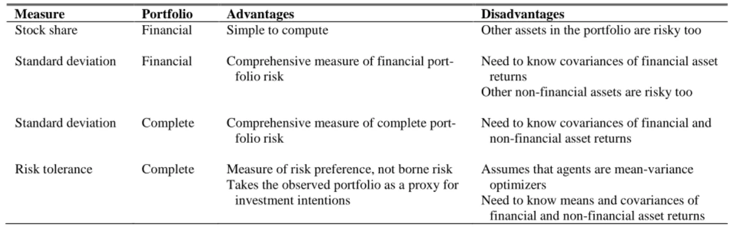
We consider four alternative indicators of risk taking, whose main features are summarized in Table 1. It should be noticed that all the four measures are derived from observations on household portfolio holdings at market value, which we assume reflect investors’ choices. This assumption may be violated for households who had chosen their portfolio composi-tion in earlier years, and then just kept it with no or limited adjustment (see, e.g., Calvet et al., 2009). For such households we would then observe the original portfolio composition modified by the different historical realizations of the asset returns.

TABLE 1 ABOUT HERE

3.1. Stock share in financial portfolio

Following the standard literature on risk, the first indicator is the share of the financial port-folio held in stocks. More generally, consider an economy with one risk free asset and a set of m risky assets. For each household ,i i=1,...,N observed at time t, we know the weights of its portfolio, ωit =ωit,1 ωit,2 … ωit m, ′. Our measure of risk is the asset share ωit s, ,

where the index s denotes stocks. In our application, m=2 and we consider (corporate and government) bonds and stocks as risky assets.

Although popular for its simplicity, this measure ignores that other risky assets apart from stocks are included in a household’s portfolio and that risk may vary over the years. This assumption is probably wrong, as testified by the recent crisis of the financial markets. For instance in a financial portfolio, bonds may be subject to firm-specific risk (corporate bonds) or country-specific risk (government bonds).

3.2. Standard deviation in financial portfolio

Our second measure acknowledges for this by computing the standard deviation of returns in the financial portfolio. More generally, let us suppose that we know for the n risky

as-sets their variances and covariances, collected in the matrix Σt. For each household

, 1,...,

i i= N observed at time t, we then compute the portfolio standard deviation

(

)

1 2

it it t it

This measure provides a thorough assessment of the risk in a financial portfolio at the cost of knowing the variances and covariances of returns among financial assets. Moreover, it may not reflect the overall household portfolio risk; in fact, it ignores that other non-financial assets – which often account for a large amount of total wealth – are risky as well.

3.3. Standard deviation in complete portfolio

We then extend our definition of portfolio, and consider an economy with one risk free as-set and a as-set of n>m risky assets, of which we know the variances and covariances, Σ_t at time t. For each household ,i i=1,...,N at time t, we observe the weights of its portfolio,

,1 ,2 ,

it it it it n

ω ₌_ω ω ω _′

… . In particular, we consider as risky assets bonds and stocks

(our financial portfolio), plus human capital, business wealth, real estate, and related liabili-ties; for sake of simplicity we group liabilities in the same category as bonds. We call this new portfolio, which includes n=5 assets, “complete portfolio”.

Real estate is certainly less liquid than financial assets, due to transaction costs; in addi-tion, most of it is residential housing and is therefore constrained to consumption needs. Similar arguments may be made on the degree of liquidity in human capital and business wealth. In a short time horizon these assets may be seen as completely illiquid, which means that their holdings cannot be changed and are taken as exogenous in the portfolio choice problem (Flavin and Yamashita, 2002). Let us then distinguish the portfolio weights for household ,i i=1,...,N at time t, ωit, in two components,

u c it it it ω ₌ω _′ ω_′′   . Weights , u i t

ω include all the holdings of unconstrained risky assets (bonds and stocks), whereas weights ,

c i t

ω include all the holdings of constrained assets (real estate, business wealth, and human capital). Accordingly we distinguish the components of the covariance matrix Σ_t in

uu uc t t t _{uc cc} t t _{Σ Σ}  Σ =  ′ Σ Σ     .

It can be shown (see Gourieroux and Jouneau, 1999, for details) that the overall portfolio variance is the sum of an unconstrained variance and a constrained variance,

| | |

u c uu u c c cc u c

it t it it t it it t it

where tcc u| cct uct

( )

uut 1 uct

−

′

Σ = Σ − Σ Σ Σ and the unconstrained weights are (1) ωitu c| ωitu

( )

uut 1 uct ωitc

−

= + Σ Σ .

Our third measure of risk is

(

)

1 2

| | |

u c u c uu u c

it it t it

σ = ω ′Σ ω , that is, the standard deviation of the unconstrained portfolio returns. This measure differs from the one based on the financial portfolio because it depends through u c|

it

ω not only on the observed portfolio weights of the financial (unconstrained) assets, but also on their covariance with the weights of the con-strained assets (hedging term). Notice that the variance of returns on the concon-strained assets plays no role in this measure.

Similarly to the standard deviation of the financial portfolio, this measure provides a comprehensive assessment of household portfolio risk, provided that one knows the va-riances and covava-riances of returns on financial assets, and the covava-riances between returns on financial and non-financial assets.

3.4. Risk tolerance implicit in complete portfolio

So far, we described households’ portfolio decisions in terms of portfolio shares and wil-lingness to bear risk, where the latter coincides with the “ex ante” standard deviation of their portfolios. However, the relationship between borne risk (measured by portfolio va-riance) and risk attitude is not straightforward. Thus, any inference about household risk at-titude exploiting data on household portfolio risk requires further simplifying assumptions. In what follows we postulate that households are myopic mean-variance (MV) optimizers (i.e. they have a one-year planning horizon) and asset returns are correlated with each other in a given time period, but they are distributed independently over time. We therefore fol-low Bucciol and Miniaci (2011), who suggest to estimate household’s risk tolerance as the one which equalizes the variance of the observed household portfolio and the variance of MV efficient one.

Our risk tolerance estimate is the value of γ_it implicit in the following equation, which imposes an identity in the variance of the returns on two portfolios:

where the variance on the left-hand side of the equation refers to the observed portfolio, and the variance on the right-hand side refers to the MV optimal portfolio, conditional on the household-specific risk tolerance γ_it and some equality and inequality constraints to their portfolio allocation, described for a generic portfolio of weights w by the conditions

Aw=b Cw≤d.

In our empirical analysis we consider equality constraints on the non-financial assets – that is, we set as exogenous the holdings of business wealth, real estate and human capital – and inequality constraints on the financial assets – short-selling restrictions on deposits and stocks, and debt below the collateral (the sum of business wealth and real estate). With this choice of the equality constraints, equation (2) is equivalent to the comparison between un-constrained variances:

( )

( )

| | | | u c uu u c u c uu u c it t it w it t w it ω ′Σ ω = γ ′Σ γ .

In general, the presence of inequality constraints prevents one from obtaining a closed-form expression for γit; see Bucciol and Miniaci (2011) for further details. The solution is then

found numerically with quadratic programming.2

One could argue that there is no specific reason to derive risk tolerance from portfolio variances, and we could also look at, for instance, portfolio expected returns. In general, any portfolio along the efficient frontier is a potential candidate for our comparison. How-ever, there are three reasons that make us opt for variances: first, the variance of an ob-served portfolio is a clear indicator of the household’s willingness to bear risk; second, it is more robust to estimation errors than the expected return (see, e.g., Merton, 1980; Chopra and Ziemba, 1993); third, our approach is consistent with the analysis in terms of Certainty Equivalent Returns (CER) from standard expected utility theory (as in Calvet et al., 2009). In fact, equation (2) is also the first order condition from the minimization of the distance between the expected utility under the observed portfolio and the expected utility under the optimal portfolio, where the utility is either the one in the MV framework, or the CRRA utility function; Bucciol and Miniaci (2011) derive this formally.

2 _{In the absence of any constraint, the risk tolerance estimate would differ from the variance of the complete}

portfolio only for the market performance,

(

1

)

1 2

it it t it t t t

γ ₌ ω ω η_{′Σ ′Σ}−η _{, with}

t

η vector of excess returns ex-pected at time t.

This measure of risk has two main advantages compared to the alternatives discussed above. First, it provides an assessment of risk attitude rather than merely borne risk. In fact, we believe it is not possible to investigate risk attitude without comparing the risk of a port-folio with its expected return. Second, it is not linked to the observed portport-folio holdings with a one-to-one relationship; observed portfolios matter only in their relation with the op-timal portfolios. They are then seen as a proxy for the real investment intentions, from which they may differ because of i) infrequent rebalancing, which means that portfolios vary just because of gains/losses in asset prices and ii) market imperfections (e.g., mini-mum investment size). The disadvantages of this measure are that it imposes the MV framework, and it needs to know not only variances and covariances of asset returns, but also their expected returns.

4. Data

4.1. Household portfolios

There are few surveys potentially useful to investigate how US households change their portfolio along the life-cycle. The Panel Study of Income Dynamics (PSID) is comple-mented by a Wealth Supplement run from 1984 to 1995 every five years, and every two years since 1999. The PSID is a longitudinal dataset, and thus it enjoys the typical advan-tages of panel data. However, with its information on assets holdings it is not possible to clearly identify the investment in composite assets such as pension funds and retirement plans, and therefore to assess how risky the portfolio is. Portfolio description is more de-tailed in the Health and Retirement Study, which is also a longitudinal study, but it focuses on the population over the age of 50. An obvious candidate dataset for our purpose is there-fore the US Survey of Consumer Finances (SCF).

The SCF is a repeated cross-sectional survey of households conducted every three years on behalf of the Federal Reserve Board. It collects detailed information on assets and liabil-ities, including home ownership and mortgages, together with the demographic characteris-tics of a sample of US households. The survey deliberately over-samples relatively wealthy households to produce more accurate statistics; in our analysis we then use the sampling weights provided by the SCF to obtain unbiased statistics for the US population. The SCF also handles the high rate of item non-response typical of wealth-related microdata by

im-puting a set of five values that represent a distribution of possibilities. Multiple imputations of missing data increase the efficiency of estimation, allowing the researcher to use all available information, and have the distinct advantage of providing information on uncer-tainty in the imputed values. We exploit this information as suggested in Rubin (1987); we develop our analysis independently for each of the five completed datasets and our final statistics are the average of the estimates derived for each dataset; standard errors account for the variability both within and between these five datasets.

Our data on household portfolio holdings are taken from the waves from 1998 to 2007 of the SCF.3 Our final sample consists of 15,134 households with head aged between 25 and 90. We consider two definitions of portfolio. The “financial” definition includes the main financial assets, grouped in three categories: deposits (that we treat as risk free), bonds, and stocks. The “complete” definition also includes human capital, business wealth, real estate, and related liabilities.4 We include liabilities in the bond category, while the other three as-sets form new categories. Human capital is estimated conditional on age, gender, race and education of the household head using an approach similar to Jorgenson and Fraumeni (1989). In a nutshell, it is a discounted projection of the future realizations of gross income, for the head and the spouse (if any); see Appendix A for details.

Over the period we consider the size of household wealth (in 2007 USD) rose markedly using either definition. The median value of financial wealth goes from 22,500 USD in 1998 to 31,000 USD in 2007, the corresponding values for the complete definition of wealth are 1,181,687 USD in 1998 and 1,916,679 USD in 2007. Wealth was indeed fueled by a rising stock market between 1998 and 2001, and by a rising house price market be-tween 2004 and 2007.

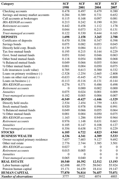
Each asset is classified as defined in Table 2, which also reports the composition of the aggregate complete portfolio, computed accounting for multiple imputations and sampling weights. The financial portfolio includes all the assets in the deposits, bonds, and stocks

3 _{We neglect wave 1995 because portfolios happen to be largely different from those observed in later waves,}

as they are more highly concentrated in deposits. We believe that including this wave would bias our analysis as its portfolios would merely reflect a change in the set of investment possibilities. For instance, 401(k) and other retirement assets were not yet widespread in 1995. We neglect previous waves of the SCF because of small changes in the questionnaire.

4 _{In a robustness check (not reported) we also included credit card debt and debt for other reasons (such as}

student loans or loans for car purchase) . Credit card was taken as a separate asset category because its returns are markedly different from those on other liabilities. Results do not change qualitatively, primarily because credit card debt weighs relatively little in most household portfolios, and we omit this case from the analysis.

categories of the complete portfolio, therefore excluding mortgages and other liabilities. Notice that the largest share in the aggregate portfolio is by far human capital (between 75% and 78%); this share is roughly in line with simulation studies in Cocco (2005). In ag-gregate human capital falls over the years because of population ageing (the economy is progressively more populated by older people, who hold less labor human capital) and be-cause in the period under investigation it provided lower returns than financial wealth (over the years 1998-2001) and real estate (2004-2007). The second largest share of wealth is held in real estate (between 10% and 13%), mostly in owner-occupied residential housing. The inclusion of mortgages in the bonds class determines an aggregate short position in it. Finally, notice that most financial wealth is held in stocks.5

TABLE 2 ABOUT HERE

There is no exact correspondence in the questions of the various SCF waves, as for stance before 2004 we have no information on the fraction of balanced composite assets in-vested in stocks. For this reason imputations have been made.6 However, the trend shown by these assets in the imputations before 2004 (with more wealth held in deposits and less in stocks) is consistent with the trend observed in other assets whose definition has re-mained constant across the waves (e.g., saving and money market accounts, directly held stocks, etc.).

To better understand the evolution of portfolio decisions over the life-cycle, we group our observations by cohorts. Specifically, we define cohorts within a range of 5 birth years. Our sample contains 15 such cohorts, born between 1910 and 1984. Since the oldest and the youngest cohorts are built from few observations, in the following figures we will show cohort-specific statistics based on at least 100 observations.

We start with the cohort-specific age profile of wealth. For each cohort and for each wave we compute aggregate wealth as the average wealth holdings in the sample, weighted

5 _{For instance, the share of stocks in the aggregate financial portfolio of 2007 is 4.94 /(2.79 +2.22 +4.94) =}

49.65%, where 2.22 is the total amount of (directly and indirectly) owned bonds (excluding liabilities).

6 _{With composite assets we mean the four assets written in Italics in Table 2 (IRA-KEOGH accounts,}

retire-ment accounts, annuities, trust-managed accounts); balanced composite assets account for about 30% of the wealth held in these assets. We then exploit information from a question on the composition of these assets and, depending on the answer we observe, we split the holding equally in deposits and stocks, bonds and stocks, or deposits, bonds and stocks.

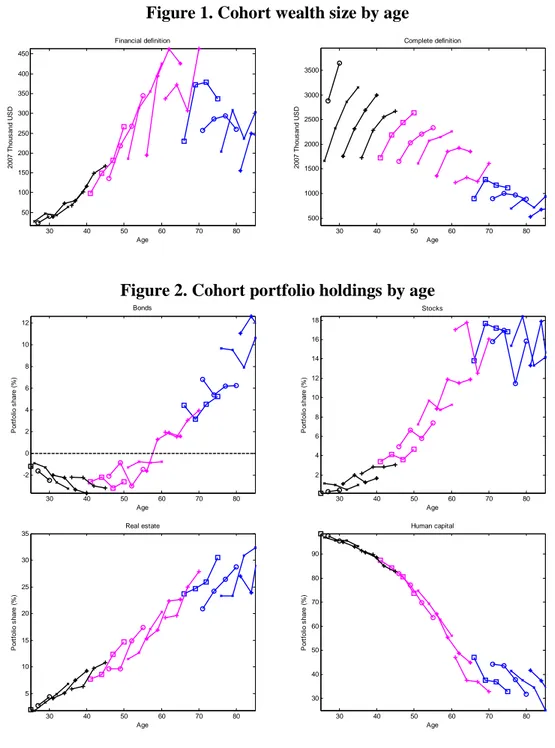
using the SCF sampling weights. Figure 1 shows the resulting age profile for the financial definition (left panel) and for the complete definition (right panel) of wealth. Values are re-ported in 2007 USD using the Consumer Price Index for all urban consumers (source: US Bureau of Labor Statistics). The figure shows for financial wealth the typical inverted U-shape profile, with remarkable cohort and time effects, with younger cohorts systematically richer than older ones. In contrast, total wealth falls monotonically with age, because hu-man capital progressively decumulates.

FIGURE 1 ABOUT HERE

We then turn our attention to the single asset holdings. Figure 2 reports the age profile of some key asset holdings for our complete definition of portfolio. Cohort portfolios are con-structed as the aggregate portfolios from the (weighted) observations in our sample and conditional on cohorts and age (see Poterba and Samwick, 1997). Most of the variation in portfolio allocation is driven by human capital, which accounts for nearly 100% of wealth at the beginning of economic life and then it markedly falls with age, leaving all the other asset shares rise. The remaining age variation in portfolio allocation seems driven by the timing of housing investment. With volatile house prices, the insurance motive makes young households purchase their house early in life (see Sinai and Souleles, 2005 and Banks et al., 2010a). In order to increase their housing consumption they resort to debt.7 It is worth noticing that the stock share is increasing more markedly only when the negative bond position is decreasing. That is, debt positions primarily due to real estate investment make stock investment less attractive. This evidence is consistent with Becker and Shabani (2010) who find that households with mortgage debt are 10 percent less likely to own stocks and 37 percent less likely to own bonds compared to similar households with no out-standing mortgage debt.

Later in the life cycle, households are expected to downsize their housing investment. However, older households do not switch from homeownership to renting. Thus, if they re-duce their position in primary residence, they do so by moving to a smaller, but still owned, house. This finding is consistent with Banks et al. (2010b), who show that the five year

7

housing transition rate from owner to renter is only 4.3% for the US homeowners over 50 years old.

FIGURE 2 ABOUT HERE

4.2. Asset time series

Information on asset returns is essential to estimate our measures of standard deviation and risk tolerance. We take annual financial returns (bonds and stocks) from the “Merrill Lynch US Corporate & Government Master Index” and “MSCI USA Stock Index” time series of US asset total return indices (downloaded from Datastream). We consider as risk free return for deposits the yield of 3-month T-bills. Annual returns for business wealth are proxied with proprietor’s income from Bureau of Economic Analysis (BEA) . To measure the un-certainty related to human capital we construct from BEA data a time series of labor in-come consistent with the definition we used in the SCF.8 Our time series cover quarterly the years from 1979 to 2007. To compute the correlations with the asset excess returns we sub-tract from this series the series of our risk free returns.

It is more problematic to find a time series of real estate returns valid for our purpose. From the perspective of a household, we need a series that accounts for not only capital gains, but also earnings due to rents. We therefore combine a repeat-sale, purchase-only in-dex calculated for the whole of the US from the Federal Housing Finance Agency (FHFA), with an estimate of imputed rents-price ratios for the US market calculated in Davis et al. (2008). The rent-price ratio decreased between 1979 and the second quarter of 2006 from 4. 85% to 3.64%, and started rising again in the following years. The average ratio in our sample period is 4.76%, in line with rough estimates in Flavin and Yamashita (2002) and Pelizzon and Weber (2008).

In the analysis, we consider a moving 20-year window (80 observations) for asset re-turns. Specifically, for the survey data collected in year X we assume that portfolio deci-sions are based on asset returns observed between year X-19 and year X. Households

8 _{See Appendix A. We take the difference between personal income and earnings from rents, dividends, and}

capital gains. The resulting time series incorporates wage and salary disbursements, supplements to wages and salaries, proprietors’ income with inventory valuation and capital consumption adjustments, and personal current transfer receipts, less contributions for public social insurance. BEA data refer to the whole US popu-lation, and thus they already incorporate unemployment spells.

viewed in different years have therefore different expectations about future market move-ments. Table 3 shows the main statistics of the asset returns we consider in the analysis.

TABLE 3 ABOUT HERE

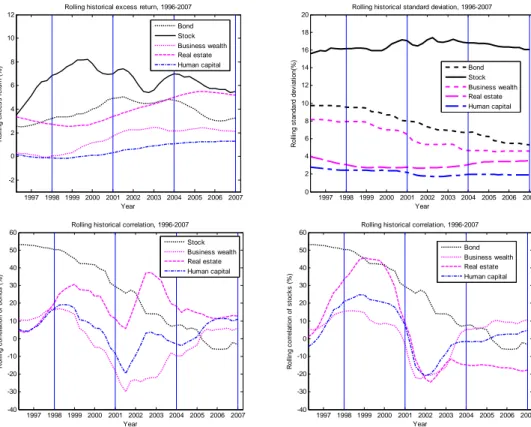
Figure 3 also informs on the results of this estimation exercise. The two top panels re-port the rolling excess return (top-left panel) and rolling standard deviation (top-right panel) for each asset from 1998 to 2007; the vertical lines show the data points we use in each wave. We see that expected stock excess returns rise dramatically before 2000, and become less predictable afterwards; bond excess returns grow until 2001, while real estate excess returns keep growing from 1999 to 2006, outperforming bonds since 2004. This is reflected in Figure 2, where stock shares systematically show a marked growth between the first and the second point of the curve for each cohort. The fall we instead observe in the age profile of stock shares between the third and fourth point of the curve for each cohort (that is, be-tween 2001 and 2004) reflects the shift of savings toward real estate, following the increase over this period in the returns of real wealth. Standard deviations are – unsurprisingly – more stable over time, but nevertheless, bond risk witnesses a remarkable reduction starting from year 2000. In order to assess the riskiness of household portfolios we also need to eva-luate the correlations between assets. The two bottom panels of Figure 3 show the rolling estimates of the correlation between bonds (bottom-right panel) and the other assets (bot-tom-left panel), and between stocks and the other assets. The two panels suggest a marked change in correlation over the years; in particular, the correlations between bonds and stocks were markedly higher at the beginning of our sample period. As a consequence, al-though the standard deviations of the returns are quite stable over time, the risk of a fixed portfolio can vary considerably due to the fluctuations of the correlations.

FIGURE 3 ABOUT HERE

We conclude this section by showing how observed portfolios perform in a MV space. Figure 4 reports this graphical analysis; the left panel refers to our financial definition, while the right panel is based on the unconstrained weights (1) of our complete definition.

Both panels suggest wide heterogeneity of portfolio decisions, with many portfolios per-forming worse than others.

FIGURE 4 ABOUT HERE

As in the empirical exercise we rely on macroeconomic time series in order to assess the riskiness of human capital, business wealth and real estate, one might argue that we are un-der-estimating these risks since we completely ignore the idiosyncratic component. How-ever, this is not a problem in our analysis. In fact, by imposing equality constraints on the holdings of the three non-financial assets, to matter for us is only the covariance between such assets and the remaining assets, which is likely to be driven by systematic rather than idiosyncratic risk.

5. Results

5.1. Distribution of risk taking

We start our analysis by showing statistics on the evolution of risk taking over time. The first part of Table 4 reports the measures of risk we derive from the aggregate portfolios in each SCF wave (those in Table 2), ignoring the heterogeneity in cohorts and other house-hold characteristics. The four measures agree in showing higher propensity to risk taking in the years 1998 and 2001 rather than in the years 2004 and 2007, in correspondence to the highest stock shares, high volatility of bonds and stocks and high correlation between bonds and stocks. Only the risk tolerance indicator reports markedly higher risk taking in 2001 than in 1998.

The second part of Table 4 shows the median value of risk taking as measured from household portfolios. The statistics thus account for the heterogeneity in household portfo-lios, especially regarding participation in the various asset markets. Even though the results from this exercise are quantitatively different from before (estimates are regularly smaller – especially for the stock share and the risk tolerance – because many households in the sam-ple hold poorly diversified portfolios with relatively little risk9), they qualitatively confirm

9 _{8.41% of the households in the sample hold only risk free and human capital assets; 15.44% hold only risk}

our above conclusion: propensity to risk taking was higher in 1998 and 2001. This time we find more marked reduction of risk taking in 2004 and 2007; in addition not only risk toler-ance, but also the stock share indicator reaches a clear peak in 2001.

TABLE 4 ABOUT HERE

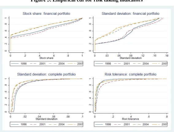
We then turn our attention to the distribution of the household-specific measures of risk. Figure 5 plots the cumulative distribution function (cdf) of our four indicators. All the measures report wide heterogeneity, reflecting different market conditions and portfolio al-location, and inform that a large part of the population has very little propensity to risk tak-ing. This is particularly evident for the stock share, that is set to 0 for a number of house-holds between 40% and 50% of the sample in the same year. Notice that the cdfs referring to the waves 2004-2007 are typically drawn above the cdfs for the waves 1998-2001, which means that over those years the distributions are shifted toward lower levels of risk taking.

FIGURE 5 ABOUT HERE

The four indicators show a similar time trend and similar distributions of risk taking. However, they may provide different results at the single household level. Table 5 reports the correlation among our four indicators, taken as average over the four waves. The corre-lation is very high (0.92) between the two indicators based on the financial portfolio (stock share and standard deviation), and smaller (0.58) between the two indicators based on the complete portfolio (standard deviation and risk tolerance). The correlation is rather small (between 0.30 and 0.43) when we compare indicators based on the financial portfolio with indicators based on the complete portfolio. It then seems that focusing on the complete portfolio rather than the financial one may lead to different conclusions.

TABLE 5 ABOUT HERE

Figure 6 compares graphically the estimates of the households’ specific indicators, tak-ing all the four waves. We observe wide heterogeneity over any pair of measures, especial-ly when comparing estimates from financial portfolios with estimates from complete

port-folios. This all suggests that the choice of the risk taking indicator is not irrelevant at the household level, since each indicator captures different aspects of risk taking.

FIGURE 6 ABOUT HERE

5.2. Age profile

In this section we investigate the correlations between our measures of risk, age and other household characteristics, time and cohort effects. For this reason we run four quantile re-gression analyses, one for each measure, where the dependent variable is our risk taking in-dicator. The specification includes five sets of explanatory variables, on wealth, demo-graphics, financial sophistication, self-assessed measures, age, cohort, and time effects. In the set of wealth variables we consider the logarithm of financial wealth, and the levels of income, real estate plus business wealth net of debt, and debt; the levels are then divided by financial wealth. In the set of demographic variables we treat dummy variables for race, gender, education, children (yes or no), marital status, and occupational status (employed, self-employed) of the household head. This specification is similar to the one in Sahm (2007)10, who estimates risk tolerance from hypothetical questions in the US Health and Retirement Study. In the same vein as Guiso and Jappelli (2005), we further include in the specification some proxies for financial sophistication: the number of financial institutions the household is involved with, and two dummy variables. The dummies are worth one re-spectively if there is regular consulting of a professional financial advisor, or the head works in the finance sector. We also include two dummy variables for the self-assessed good or excellent health status of the head, and for the self-assessed degree of optimism of the household.11

We finally add variables meant to disentangle time and cohort effects from age effects. After trying alternative specifications, we choose one where age effects are captured with dummy variables covering a five-year age range (the baseline is age 25-29), time effects are measured with the average excess return of the stock market in the three years prior to the

10 _{Sahm (2007) focuses on cash-on-hand (wealth plus income) rather than wealth. We prefer our specification}

because cash-on-hand is highly correlated with income. For the same reason, we do not consider a measure of “life-cycle wealth” as described by the sum of wealth and human capital.

11 _{The question asks whether “the US economy will perform better, worse, or about the same in the next 5}

wave12, and cohort effects are measured with the average excess return of the stock market when the head was between 20 and 24 years old.13 This specification mimics one in Ame-riks and Zeldes (2004), where in particular the variable on the cohort effect is meant to de-scribe a “learning” process of the market behavior when young.

Table 6 shows the results of our analysis, separately for the four indicators; the size of the coefficient estimates is clearly different over the four columns, because each indicator has its own scale (see Table 4). We first focus on the two measures based on the financial portfolio definition. We find several regularities: each risk taking indicator correlates posi-tively with financial wealth, income, the number of financial institutions where doing busi-ness, and with the dummy for individuals working in the finance sector, and negatively with debt and the dummy variables for non-white and self-employed individuals. In addi-tion, we find no cohort effect and an age effect insignificantly different from zero in the ages between 45 and 70. In contrast, we observe a strong time effect. This means that, as the stock excess return in the previous three years is the highest (this happens in 1998), the risk indicator rises as well.

When we look at the two measures based on the complete portfolio definition, some – but not all – our previous findings are confirmed. We still find positive correlations be-tween our risk taking indicators and financial wealth, income, the number of financial insti-tutions where doing business, and with the dummy for the finance sector. Notice in particu-lar that we find a positive correlation between risk measures and wealth, as in Siegel and Hoban (1982) and Morin and Suarez (1983). This time we also find that risk taking is high-er among females, college graduates, individuals with self-assessed good health, and it is lower for employed workers and when the individual is optimistic about the future14; Ben

12 _{Based on our time series of stock excess returns. For instance, for year 2007 we take the average from the}

12 observations between 2005 and 2007.

13 _{Our time series of stock excess returns does not allow to retrieve this information from the oldest cohorts.}

For this reason we refer to data available in Kenneth French’s website. Specifically, we consider as excess market return the value-weight return on all NYSE, AMEX, and NASDAQ stocks (from CRSP) minus the one-month Treasury bill rate (from Ibbotson Associates).

14 _{The result that females are more risk tolerant goes against the evidence from previous works. We believe}

that this effect depends on the inclusion of non-financial assets in the definition of complete portfolios. In par-ticular, the median household with a female head holds a relatively larger portfolio weight on human capital (89.41%, as opposed to 76.04% for males). To hedge against this increase in (exogenously given) portfolio risk, the household should invest more heavily in financial assets, especially stocks; however, in our sample 54.91% of the households with a female head do not invest in stocks, as opposed to 28.62% of the households with a male head.

Mansour et al. (2008) also find a negative correlation between risk and optimism. As for the other two indicators, we find a strong time effect that is now coupled with a strong co-hort effect and an age effect always significantly different from zero, apart from the early ages up to 40.

TABLE 6 ABOUT HERE

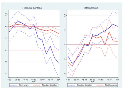
For sake of comparison we provide a graphical representation of the age effects esti-mated for the four indicators. In Figure 7 we depict the estiesti-mated age profile conditional on the median values of wealth, demographic and other household characteristics; for compa-rability reason, the profile is divided by the median observed risk taking indicator.

There is marked difference between the measures based on the financial portfolio and the measures based on the complete portfolio. The former show an age profile that is essen-tially flat up to age 60, and then falls – especially as concerns the stock share, which goes to 0 for the elderly. This evidence is somewhat more complex than common rules of thumb adopted by practitioners, e.g., to invest in stocks a fraction

(

100−age

)

% of the financial wealth. In contrast, the two measures based on the complete portfolio show an age profile that rises at young ages, up to 40, after which it becomes stable, or slightly increases further (significantly only for the standard deviation indicator). Evidence of a rising age profile is not surprising given the complete portfolio shares shown in Figure 2. In fact, the complete portfolio is largely dependent on human capital, which naturally falls with age. As individ-uals get older, their portfolios exhibit higher investment in assets that carry relatively more risk than human capital. Our indicators capture this life-cycle effect in the change of the unconstrained portfolio weights of equation (1). These weights tend to rise for two reasons. First, the portfolio shares in bonds and stocks tend to increase with age (see Figure 2); second, the term of hedging against human capital falls because the weight on human capi-tal reduces with age. Inertia in portfolio adjustment is also likely to play a role. Consider the case of a household with a given complete portfolio. If this household does not inter-vene on her portfolio composition, and the market provides the same returns to all the as-sets, after three years the household holds lower human capital. We then observe a relative-ly larger investment in bonds and stocks, which is used to hedge against a risk that is lower than in the previous three years (since there is less human capital). This situation makes the

household look more risk tolerant now than in the past. This household may thus bear more risk even if her attitude toward risk taking is the same as in the past.

FIGURE 7 ABOUT HERE

5.3. Sensitivity analysis

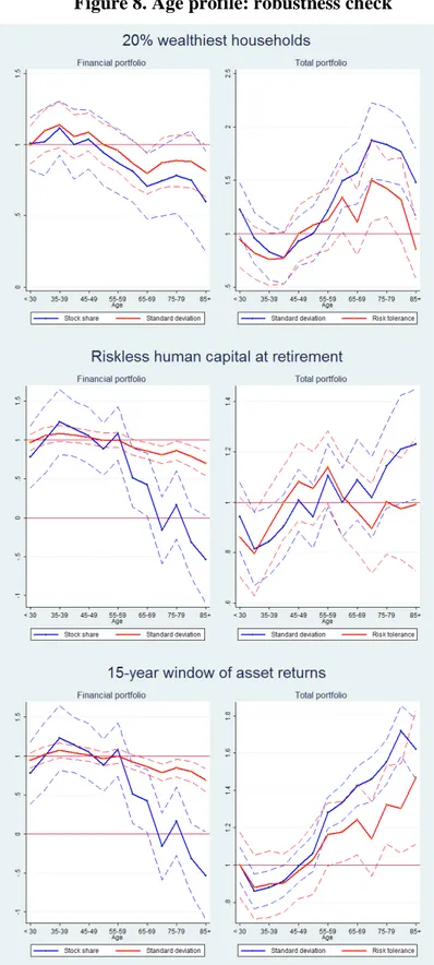
The results obtained so far show that: (i) the way risk varies with age depends on the defini-tion of portfolio, (ii) risk taking is positively correlated with wealth, income and financial sophistication, and (iii) business cycle (captured by financial markets indexes) helps ex-plaining heterogeneity in household portfolio volatility and risk attitudes. In this section we run some robustness checks. Methodological details and complete regression results can be found in the Supplementary Appendix; here we only comment the relevant findings and show Figure 8 with the estimated age profiles of the four measures.

FIGURE 8 ABOUT HERE

Transaction costs

What we interpreted as heterogeneity in risk borne by the households, and thus as hetero-geneity in risk tolerance, might in fact be due to heterohetero-geneity in transaction costs (see Bucciol and Miniaci, 2011, for a detailed discussion of the issue). It is reasonable to expect that the richer the investor the less relevant the transaction costs are for his portfolio choice. Under this assumption, if we observe that our main results hold also when we restrict the sample to the top 20% wealthiest households (which also have a higher income, are better educated and more sophisticated investors), we can be confident that transaction costs do not significantly affect our results. The sub-population of the wealthiest households has an average financial wealth which is about the triple of the financial wealth of the full sample, it invests 39.5% of it in stocks, its portfolios are riskier and their estimated implicit risk to-lerance measures are higher. Nevertheless, the main results of our multivariate analysis still hold: there is a positive relation between risk taking, wealth and financial sophistication, and age, time, and cohort effects are close to those of the benchmark case. However, in this case the confidence interval associated to the age effect is larger and we cannot exclude that the willingness to undertake risk is constant with age (see Figure 8, first panel).

Riskless human capital at retirement

In our main analysis we treat human capital from pension income exactly the same way as human capital from labor income. However, it may be plausible that pension income is less risky than labor income. In this robustness check we replicate the main analysis under the extreme situation where pension human capital is riskless. Again, our benchmark results are confirmed also here; in particular the age effects show a decline after age 60 using the fi-nancial definition, and a rise up to age 40 using the complete definition (see Figure 8, second panel).

Alternative estimates of asset return moments

In our exercise we use estimates of the historical average and the variance-covariance ma-trix of asset returns. The estimates we provided so far are based on a 20-year backward ho-rizon, as described in Section 4. Alternative estimates of the expected returns and variance-covariance matrix would imply a different assessment of the portfolio risk and its corres-ponding risk taking indicators, in particular for what concerns the time effects. As identifi-cation of age, cohort and time effects are strictly related, it is relevant to check if our results change if we vary the time horizon considered for our estimates. We therefore provide new estimates in which the moments of the asset returns are estimated using 15 years instead of 2015. Shortening the estimation period affects remarkably the estimate of returns volatility and correlations. However, the multivariate analysis on household portfolios does confirm our benchmark results, and it gives rise to an age profile in line with our previous findings (see Figure 8, third panel).

6. Conclusions

In this paper we use data from the waves 1998-2007 of the US Survey of Consumer Fin-ances (SCF) to shed light on the evolution of US households’ portfolio risk, and the correla-tion between risk attitude, wealth, age and the main household socio-demographic characte-ristics. The use of repeated cross sections allows us to disentangle age effects from time and cohort effects.

In our analysis we consider four different indicators of risk taking, based on two differ-ent definitions of portfolio (financial and complete, including also human capital, real

15

tate, business wealth and related debt). The four indicators show a similar time trend with risk taking peaking in 2001, and inform that the distribution of household risk taking is skewed to the left, with many households willing to take little risk. Moreover, in all the cases we find our measures of risk taking to correlate positively with wealth, income, and some proxies for financial sophistication. However, the four indicators are imperfectly cor-related, and the correlation is particularly low when comparing a measure based on the fi-nancial portfolio with one based on the complete portfolio. As regards the age profile of risk taking, under the assumption that the other household characteristics remain fixed over the life-cycle, we also find different results when looking at the financial or complete port-folios. Using the two indicators derived from the financial portfolio, risk taking is constant up to age 60, and then it falls; using the two indicators derived from the complete portfolio, risk taking increases up to age 40, and then it remains stable. Importantly, in all the cases we find that risk taking is constant with age for a large part of the life cycle, and in particu-lar over the ages between 40 and 60.

One of the indicators we consider, the implicit risk tolerance, is conditional on the as-sumption of myopic MV optimization. Thus we do not consider that – in a MV multi-period framework – some of the portfolio heterogeneity is due to differences in the expe-rienced portfolio performance and planning horizon. We consider this paper as a first step towards a better understanding of the causality relations between risk preference, wealth and observable characteristics. Future research will develop a fully multi-period frame-work, closer to a life-cycle model of asset allocation, from which to infer risk preferences.

Appendix A. Human capital calculation

We construct human capital using an approach similar to Jorgenson and Fraumeni (1989). The approach computes human capital as the net present value of the income flow that will be produced over an assumed lifetime, in the presence of survival probabilities. Expected future incomes are predicted from the observed incomes of the cross section of individuals. An advantage of this method is that it allows to estimate human capital even for those households who report no income (398 out of 19,165 in the sample, 0.91% considering the sampling weights).

Income in the US arises from a process depending on several characteristics of the head, in particular gender (male, female), race (white, non-white) and education (high school or lower, college). We denote the realization of these three variables by group x∈X . The combination of the three variables gives rise to eight possible groups.

We describe human capital for household i at time t, whose head is aged a and belongs to group x, as follows:

( )

( )

( )

a a a

it it it

HC x = y x +LI x

where y_ita

( )

x is the gross income reported in the survey for the household head and spouse

(if any), and LIita

( )

x is imputed household lifetime gross income.

16

This measure is esti-mated from predictions of future income realizations, and it is defined as follows:

( )

,

( )

ɵ

( )

1 1 1 b a T _b a a b it it it b a t LI x x y x r π − = +   =   +  

∑

.

That is, lifetime income is the sum of the predicted income levels, ɵyb_it

( )

x , conditional on

age b and group x, weighted by a survival probability a b,

( )

it x

π of being alive at age b

condi-tional of being alive at age a and time t, for individual i belonging to group x17, and cor-rected by a discount rate (1+r_t), computed as average over the 20 years before t of real risk

free returns (3-month T-bill yields net of CPI growth).18

Income predictions up to age 64 are derived from the OLS regression of the logarithm of one plus income over a third-order polynomial on age, gender and race dummies, cohort dummies and time dummies respecting the Deaton-Paxson orthogonality constraints. In-come predictions since age 65 are the inIn-come prediction at age 64 times a replacement rate. The rate is given by the ratio of average observed income between 65 and 69 to average ob-served income between 60 and 64, and it is computed separately by education groups. In all the cases we take into account imputations and sampling weights. For households with head older than 64, predicted income is the income predicted for their class times the replace-ment rate.

16 _{On average in our data, gross income is around 4-5% of human capital.}

17 _{Actually, in our calculation survival probabilities differ by gender and not also by race or education,}

be-cause no such data are available.

18

We estimate the regression and the replacement rate19 from the SCF dataset described in Section 4.1, separately for each imputation and for each education group. As one may ex-pect, projected income is higher for households with a male, white and more highly edu-cated head.

19 _{We estimate an average replacement rate of 88.88% for high school graduates, and 71.95% for college}

gra-duates; we do not compute the replacement rate separately also by race and gender for sake of simplicity, as only education seems to matter.

References

Agnew, J., P. Balduzzi, and A. Sundén (2003), “Portfolio Choice and Trading in a Large

401(k) Plan”, American Economic Review, 93(1), 193-215.

Alan, S. (2006), “Entry Costs and Stock Market Participation over the Life Cycle”, Review

of Economic Dynamics, 9(4), 588-611.

Ameriks, J., and S. Zeldes (2004), “How Do Household Portfolio Shares Vary with

Age?”, Working Paper, Columbia University.

Angerer, X., and P. Lam (2009), “Income Risk and Portfolio Choice: An Empirical

Study”, The Journal of Finance, 44(2), 1037-1055.

Banks, J., R. Blundell, Z. Oldfield, and J. Smith (2010a), “Housing Price Volatility and

Downsizing in Later Life”, in D.Wise (ed.) Research Findings in the Economics of Ag-ing, Chicago: University of Chicago Press, 337-86.

Banks, J., R. Blundell, Z. Oldfield, and J. Smith (2010b), “Housing Mobility and

Down-sizing at Older Ages in Britain and the United States”, IZA Discussion Paper No. 5168.

Becker, T.A., and R. Shabani (2010), “Outstanding Debt and the Household Portfolio”,

The Review of Financial Studies, 23(7), 2900-2934.

Ben Mansour, S., A. Jouini, J.M. Marin, C. Napp, and C. Robert (2008), “Are Risk

Averse Agents More Optimistic? A Bayesian Estimation Approach”, Journal of Applied

Econometrics, 23(6), 843-860.

Bilias, Y., D. Georgarakos, and M. Haliassos (2009), “Portfolio Inertia and Stock Market

Fluctuations”, CEPR Discussion Paper No. 7239

Brunnermeier, M. K., and S. Nagel (2008), “Do Wealth Fluctuations Generate

Time-Varying Risk Aversion? Micro-Evidence on Individuals’ Asset Allocation”, American

Economic Review, 98(3), 713-736.

Bucciol, A., and R. Miniaci (2011), “Household Portfolios and Implicit Risk Preferences”,

Review of Economics and Statistics, forthcoming.

Calvet, L.E., J.Y. Campbell, and P. Sodini (2009), “Fight or Flight? Portfolio

Rebalanc-ing by Individual Investors”, Quarterly Journal of Economics, 124(1), 301-348.

Campbell, J. , and L. Viceira (2002), Strategic Asset Allocation: Portfolio Choice for

Long-Term Investors, Oxford: Oxford University Press.

Cocco, J.F. (2005), “Portfolio Choice in the Presence of Housing”, Review of Financial

Davis, S.J., F. Kubler, and P. Willen (2006), “Borrowing Costs and the Demand for

Equi-ty over the Life Cycle”, Review of Economics and Statistics, 88(2), 348-362.

Davis, M.A., A. Lehnert, and R.F. Martin (2008), “The Rent-Price Ratio for the

Aggre-gate Stock of Owner-Occupied Housing”, Review of Income and Wealth, 54(2), 279-284.

Deaton, A., and C.H. Paxson (1994), “Saving, Growth and Aging in Taiwan”, In D. Wise

(ed.) Studies in the Economics of Aging, Chicago: University of Chicago Press.

Draviam, T., and T. Chellathurai (2002), “Generalized Markowitz Mean-Variance

Prin-ciples for Multi-Period Portfolio-Selection Problems”, Proceeding of the Royal Society A: Mathematical, Physical & Engineering Sciences, (458), 2571–2607.

Flavin, M., and T. Yamashita (2002), “Owner-Occupied Housing and the Composition of

the Household Portfolio”, American Economic Review, 92(1), 345-362.

Geanakoplos, J., M. Magill and M. Quinzii (2004), “Demography and the Long-Run

Pre-dictability of the Stock Market”, Brookings Papers on Economic Activity, 1, 241-307.

Guiso, L., M. Haliassos, and T. Jappelli (2001), Household Portfolios, Cambridge: MIT

Press.

Guiso, L., and T. Jappelli (2005), “Household Portfolio Choice and Diversification

Strate-gies”, Trends in Saving and Wealth Working Paper No. 7/05.

Heaton, J., and D. Lucas (1997) “Market Frictions, Savings Behavior, and Portfolio

Choice”, Macroeconomic Dynamics, 1(1), 76-101.

Jianakoplos, N.A., and A. Bernasek (2006) “Financial Risk Taking by Age and Birth

Co-hort”, Southern Economic Journal, 72(4), 981-1001.

Jorgenson, D.W., and B.M. Fraumeni (1987), “The Accumulation of Human and

Non-Human Capital, 1948-1984”, in R. Lipsey and H. Tice (eds.), The Measurement of Sav-ing, Investment and Wealth, Chicago: University of Chicago Press.

Kent, C., A. Park and D. Rees (Eds.) (2006), “Demography and Financial Markets”,

Pro-ceeding of a G20 conference held in Sydney on 23-35 July 2006, Australian Govern-ment Treasury and Reserve Bank of Australia.

Lusardi, A., and O. Mitchell (2007) “Baby Boomer Retirement Security: The Roles of

Planning, Financial Literacy and Housing Wealth”, Journal of Monetary Economics, 54(1), 205-224.

McInish, T.H. (1982), “Individual Investors and Risk-taking”, Journal of Economic

Psy-chology, 2(2), 125-136.

Morin, R.A., and A.F. Suarez (1983), “Risk Aversion Revisited”, Journal of Finance,

38(4), 1201-1216.

Normandin, N. and P. St-Amour (2008), “An Empirical Analysis of Aggregate

House-hold Portfolios”, Journal of Banking &Finance, 32, 1583-1597.

Palsson, A. (1996), “Does the Degree of Relative Risk Aversion Vary with Household

Characteristics?”, Journal of Economic Psychology, 17(6), 771-787.

Pelizzon, L., and G. Weber (2008), “Are Household Portfolios Efficient? An Analysis

Conditional on Housing”, Journal of Financial and Quantitative Analysis, 43(2), 401-432.

Poterba, J.M., and A.A. Samwick (1997), “Household Portfolio Allocation over the Life

Cycle”, NBER Working Paper No. 6185.

Sahm, C. (2007), “How Much Does Risk Tolerance Change?”, Finance and Economics

Discussion Series No. 2007-66, Federal Reserve Board.

Siegel, F.W., and J.P. Hoban (1982), “Relative Risk Aversion Revisited”, Review of

Eco-nomics and Statistics, 64(3), 481-487.

Sinai, T. and N. Souleles (2005), “Owner-Occupied Housing as a Hedge Against Rent

Risk”, The Quarterly Journal of Economics, May, 763-789.

Takats, E. (2010), “Ageing and Asset Prices”, BIS Working papers No. 318, Bank for

In-ternational Settlements.

Viceira, L. (2001), “Optimal Portfolio Choice for Long-Horizon Investors with

Nontrada-ble Labor Income”, Journal of Finance, 56(2), 433-470.

Wachter, J.A., and M. Yogo (2010), “Why Do Household Portfolio Shares Rise in

Table 1. Alternative risk taking indicators

Measure Portfolio Advantages Disadvantages

Stock share Financial Simple to compute Other assets in the portfolio are risky too

Standard deviation Financial Comprehensive measure of financial

port-folio risk

Need to know covariances of financial asset returns

Other non-financial assets are risky too

Standard deviation Complete Comprehensive measure of complete

port-folio risk

Need to know covariances of financial and non-financial asset returns

Risk tolerance Complete Measure of risk preference, not borne risk

Takes the observed portfolio as a proxy for investment intentions

Assumes that agents are mean-variance optimizers

Need to know means and covariances of financial and non-financial asset returns