Soft sensing in the process industry

Università Politecnica delle Marche

Scuola di Dottorato di Ricerca in Scienze dell’Ingegneria Curriculum in Ingegneria Industriale

---

Soft sensing in the process industry

Ph.D. Dissertation of:

Edoardo Copertaro

Advisor:

Prof. Gian Marco Revel Curriculum supervisor: Prof. Nicola Paone

Abstract

Present contribution discusses the application of soft sensing in the process industry, as an indirect monitoring technique for the on-line assessment of non-accessible process variables. A relevant application case is presented which involves clinker sintering, a low-efficient, high-energy intensive process with strong environmental impact: the soft-sensing approach is firstly tested in the conventional thermal system, then it is addressed an innovative heating module based on the application of high-power, mono-modal microwaves to the material under processing.

The work is focused over the development of physical models for the indirect evaluation of the critical process variables. The integration of the computation routines with the data provided by the sensors of the monitoring architectures is also addressed, as well as possible optimization strategies for improving the reliability of the tools.

A stochastic method based on an adaptive Monte Carlo procedure is implemented, for assessing the propagation of the input uncertainties through the mathematical model of the soft sensor. An innovative numerical framework provides a lower-bound estimation of the uncertainty introduced by the model itself. Successively, the overall uncertainty of the soft sensor is calculated as the composition of the different contributes.

The soft sensors are tested in the real-time monitoring of thermal and chemical variables of the processes considered. The indirect estimations of the target variables are compared with direct measurements, showing deviations in the order of 1%. Computation routines ensure fast executions, thus improving the exploitability of the tools. Results confirm the good performances of the soft sensors in the on-line monitoring of non-accessible variables. The intrinsic robustness makes them a potential back-up of direct sensors, ready to intervene when a breakdown of the hardware counterpart occurs, and before this affects the process.

Contents

List of Figures ... ii

List of Tables ... iv

Introduction ... 1

Section 1 – Soft sensing ... 3

1.1 – Literature survey ... 3

1.1.1

– Data-driven soft sensors ... 4

1.1.2 – Model-driven soft sensors ... 5

1.2 – The concept of soft sensing ... 6

1.3 – Soft sensors vs. hardware sensors ... 7

1.4. – Estimation of the uncertainty of a soft sensor ... 9

1.4.1 – Propagation of input uncertainties through the correlating model .... 9

1.4.2 – Uncertainty introduced by the correlating model ... 10

Section 2 – Clinker production process... 11

2.1 – Conventional thermal process ... 12

2.1.1 - Quarrying ... 12

2.1.2 – Raw mixture preparation ... 13

2.1.3 - Clinkering ... 13

2.1.4 – Cement grinding ... 14

2.2 – New microwave heating stage ... 15

Section 3 – Soft sensing for conventional rotary kilns ... 17

3.1 – The real kiln ... 18

3.2 – CFD-FEA model ... 20

3.2.1 – CFD analysis of the freeboard region ... 21

3.2.2 – Transport and diffusion of pulverized fuel with the primary air ... 22

3.2.3 – Fuel oxidation ... 22

3.2.4 – Propagation of radiation inside the freeboard region ... 23

3.2.5 – Radiative, convective and conductive heat exchanges between the

freeboard gas, the material bed and the wall ... 23

3.2.6 – Heat conduction inside the wall and the material bed ... 23

3.2.7 – Chemical conversion of the material bed ... 24

3.3 – Lumped element model ... 25

3.4 - Results ... 33

3.4.1 – CFD-FEA model ... 33

3.4.2 – Optimized lumped element model ... 41

Section 4 – Estimation of the uncertainty of the soft sensor ... 48

4.1 – Propagation of the input uncertainties... 48

4.2 – Extended Discrete Element Method ... 50

4.2.1 – DEM approach for the powder phase ... 50

4.2.2 – CFD approach for the fluid domain ... 53

4.2.3 – DEM-CFD coupling ... 55

4.3 – XDEM model ... 55

4.4 - Results ... 56

4.5 – Uncertainty introduced by the model ... 67

Section 5 – Soft sensing for the new microwave heating stage ... 70

5.1 – Monitoring architecture of the new DAPhNE module ... 70

5.2 – Lumped element model ... 71

5.3 – Input measurements ... 73

5.3.1 – Electrical absorbance ... 74

5.3.2 – Absorbed and back-reflected power ... 74

5.3.3 - Temperature ... 75

5.4 - Results ... 80

Concluding Remarks ... 84

References ... 86

Appendix A.1 – adaptive Monte Carlo procedure ... 92

Appendix A.2 – CFD-FEA model for the conventional rotary kiln ... 94

Appendix A.3 – LEM model for the conventional rotary kiln ... 97

Appendix A.4 – GUI for the conventional rotary kiln ... 102

List of Figures

Figure 1. The concept of soft sensing. ... 7

Figure 2. Input uncertainties of the correlating model. ... 9

Figure 3. Distributed vs. lumped element model. ... 10

Figure 4. Temperature profiles in short-dry kilns [62]. ... 15

Figure 5. Microwave cavity. ... 16

Figure 6. Loss factor vs. temperature. ... 16

Figure 7. Geometry of the kiln. ... 20

Figure 8. Mesh elements on a vertical cross-section. ... 21

Figure 9. Iterative routine for calculating chemical conversion. ... 24

Figure 10. Application of the shooting method. ... 28

Figure 11. Temperature profiles from iterative routine (continuous line) and

bvp4c (dots). ... 29

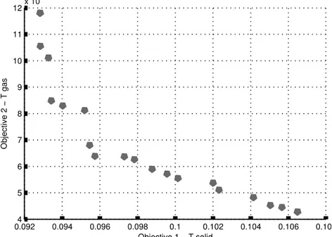
Figure 12. 2D-projection of the Pareto front. ... 31

Figure 13. LEM steady solution after optimization. ... 32

Figure 14.. Temperature profiles – comparison between LEM prediction and

CFD-FEA model. ... 33

Figure 15. x-direction velocity field (m/s) – freeboard region. ... 34

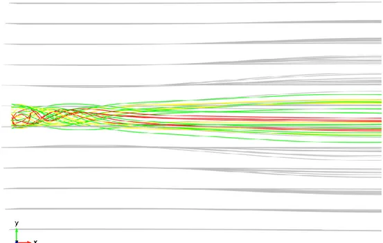
Figure 16. Streamlines – burner area. ... 35

Figure 17. logCfCf_inlet – burner area. ... 36

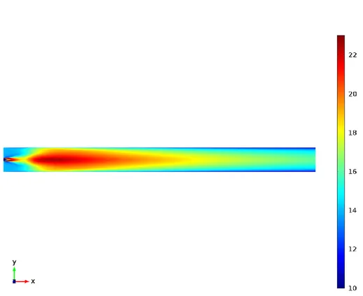
Figure 18. Temperature field (K) – freeboard region. ... 37

Figure 19. Temperature field (K) – burner area. ... 38

Figure 20. Temperature distribution of the solid material (K) ... 39

Figure 21. Temperature profiles. ... 40

Figure 22. Chemical profiles. ... 41

Figure 23. Step response after increasing the fuel flow. ... 42

Figure 24. Step response after reducing the mass flow of raw meal to 112

T/h. ... 43

Figure 25. Step response after reducing the mass flow of raw meal to 90

T/h. ... 44

Figure 26. Step response after reducing the mass flow of raw meal to 90

T/h. Rot. Speed and fuel flow are adjusted ... 45

Figure 27. Convective heat exchange – lines are for section 3.3.3 prediction,

dots for increased value. ... 46

Figure 28. Emissivity – lines are for section 3.3.3 prediction, dots for

reduced value. ... 47

Figure 30. Simulation domain (particles are not in scale). ... 56

Figure 31. Velocity field ... 57

Figure 32. CFD-DEM coupling... 58

Figure 33. Positions vs. time. ... 59

Figure 34. Temperature distribution – t=1 min. ... 60

Figure 35. Temperature distribution – t=10 min. ... 61

Figure 36. Temperature distribution – t=20 min. ... 62

Figure 37. CaO distribution – t=1 min. ... 63

Figure 38. CaO distribution – t=10 min. ... 64

Figure 39. CaO distribution – t=20 min. ... 65

Figure 40. C2S distribution – t=20 min. ... 66

Figure 41. C3S distribution – t=20 m ... 67

Figure 42. Probability distributions of temperature. ... 68

Figure 43. Temperature vs. time. ... 69

Figure 44. DAPhNE monitoring infrastructure. ... 71

Figure 45. Calibration of the h

coefficient using IST model as reference. 72

Figure 46. Graphical User Interface. ... 73

Figure 47. Incident, absorbed and back-reflected power components. ... 74

Figure 48. Absorbed to incident power ratio. ... 75

Figure 49. Measurement setup. ... 76

Figure 50. Alumina emissivity spectrum [98]. ... 76

Figure 51. Coating emissivity spectrum at 300 °C. ... 77

Figure 52. IR measurements with (b) and without (a) the high-emissivity

coating. ... 77

Figure 53. Experimental setup for the estimation of emissivity. ... 78

Figure 54. Measurements from pyrometer and contact sensor. ... 79

Figure 55. Temperature measurements during operation. ... 79

Figure 56. Thermal image from the outside of the cavity. ... 80

Figure 57. Maximum temperature of the material vs. time. ... 81

Figure 58. Prediction from the soft sensor and direct measurement from the

IR camera for the maximum temperature of the material. ... 82

List of Tables

Table 1. Chemical composition of clinker. ... 11

Table 2. Particles size distribution of raw meal. ... 13

Table 3. Thermo-physical properties of fuel and the material bed. ... 19

Table 4. Chemical composition of fresh raw meal. ... 19

Table 5. Measurements. ... 20

Table 6. Initial mass fractions. ... 25

Table 7. Reactions involved in clinker sintering [80]. ... 27

Table 8. Variation ranges for the input parameters. ... 30

Table 9. Parameters of the GA optimization. ... 30

Table 10. LEM steady solution compared to measurements. ... 31

Table 11. Mono-variant sensitivity analysis. ... 48

Introduction

In the process industry disposing of accurate measurements of critical variables at the appropriate sampling frequency is fundamental in order to take proper control actions. On this regard, hardware devices may not satisfy fundamental requirements, mainly in terms of reliability and performances. In either case on-line control and optimization schemes cannot be implemented.

Recently, new indirect measurement approaches based on soft sensing have gained relevance in the field of process monitoring, whereas technical or economic aspects make hardware devices unsuitable. In this sense, disposing of theoretical models based on the phenomenological knowledge of the process and/or on regression analyses of the historical data, allows the full exploitation of a large number of values measured continuously as they may represent input signals for the soft sensor. At the same time, soft sensing opens the way to a wide range of applications, among which on-line monitoring, process fault detection, identification of broken sensors and back up of the hardware equipment.

Present contribution discusses the general application of soft sensing in the process industry. An application case is presented, regarding the clinker production process. Indeed, this process is deeply affected by a dramatic lack of direct measurements on critical variables, as a consequence of technical difficulties (aggressive environment, physical inaccessibility, moving parts, etc.). Lack of measurements prevents the achievement of a full understanding of the process thus resulting in non-optimized operation. Soft sensing could represent a valuable tool for filling this gap of knowledge and producing new efficiency-oriented control strategies, which is an actual issue for whole the global cement industry.

The manuscript is organized as follows:

I. Section 1 introduces the topic of soft sensing. In subsection 1.1 a literature survey is reported, concerning the application of indirect measurement techniques to the monitoring of industrial processes: the development approach of a soft sensor is discussed; potentialities and weaknesses are identified; further, a wide range of applications is reported. Subsection 1.2 describes the concept of soft sensor, and provides deep focus on both its metrological and theoretical aspects. Subsection 1.3 points out the differences between a soft sensor and the hardware counterpart; it deals with the distinction between the theoretical model supporting a soft sensor and the transduction function of a measurement device. Subsection 1.4 is concerned over possible methods for esteeming the uncertainty of a soft sensor, which is a topic not faced yet.

II. Section 2 introduces the clinker production process. Particular focus is dedicated to the kiln system, a high-energy intensive, low-efficient sintering stage with strong environmental impact. Subsection 2.1 deals with the conventional thermal process, whilst subsection 2.2 is focused over an innovative heating cavity developed in the EU FP7 project DAPhNE (grant agreement n° 314636), which is based on microwaves application.

to be in good agreement with real data; besides, it represent valuable information to be used in the development of new optimization-oriented control strategies. IV. In section 4 the accuracy of the soft sensor is esteemed by studying the propagation

of the input uncertainties through the mathematical model; further, an innovative modellistic framework is used for quantifying the approximation introduced by the simplifying assumptions of the theoretical part.

V. In section 5 an analogous monitoring approach is proposed for the new DAPhNE module. The possibility for intervening in the design of the whole monitoring architecture has been fully exploited for integrating the new tool with the rest of the hardware devices.

Section 1 – Soft sensing

1.1 – Literature survey

In the last two decades, soft sensors have established themselves as a valid alternative to traditional approaches for monitoring critical process variables, whereas technical or economic aspects make direct measurements unfeasible. According to Kadlec [1], “industrial processing plants are usually heavily instrumented with a large number of sensors. The primary purpose of the sensors is to deliver data for process monitoring and control. But approximately two decades ago researchers started to make use of the large amounts of data being measured and stored in the process industry, by building predictive models based on this data. In the context of process industry, these predictive models are called “soft sensors”. This term is a combination of the words “software”, because the models are usually computer programs, and “sensors”, because the models are delivering similar information as their hardware counterparts”.

According to Mohler [2], “control systems and optimization procedures require regular and reliable measurements at the appropriate frequency […]. The quality measure may only be available as a laboratory analysis or very infrequent on-line measurement”. Lack of appropriate on-line instrumentation and unreliability of on-line instruments are mentioned as possible causes which may prevent the achievement of good measurements. In either case on-line control or optimization schemes cannot be implemented. As stated in [2], “the application of soft sensors for estimating hard-to-measure process values is extremely interesting in the process industry, where there are usually a large number of values measured continuously and they may serve as input signals for the soft sensor. They can work in parallel with real sensors, allowing fault detection schemes devote to the sensor’s status analysis to be implemented. Also, they can take the place of sensors which have been taken off for maintenance, to keep control loops working properly and to guarantee product specification without undertaking conservative production policies, which are usually too expensive”. In its literature survey, Kadlec [1] identifies a broad range of tasks were a soft sensor could be effectively exploited. In this sense, “the original and still most dominant application area of soft sensors is the prediction of process variables which can be determined either at low sampling rates or through off-line analysis only. Because these variables are often related to the process output quality, they are very important for the process control and management. For these reasons it is of great interest to deliver additional information about these variables at higher sampling rate and/or at lower financial burden, which is exactly the role of the soft sensors […]. Other important application field of soft sensors is fault detection […]”; on this regard “once a fault sensor is detected and identified, it can be either reconstructed or the hardware sensor can be replaced by another soft sensor, which is trained to act as a back-up soft sensor of the hardware measuring device. If the back-up sensor proves to be an adequate replacement of the physical sensor, this idea can be driven even further and the soft sensor can replace the measuring device also in normal working conditions. The software tool can

Kadlec [1] distinguishes two types of soft sensors, “namely “model-driven” and

“data-driven” soft sensors. Firsts are also called white-box models because they have full

phenomenological knowledge about the process background. In contrast to this purely data-driven models are called black-box techniques because the model itself has no knowledge about the process and is based on empirical observations of the process […]. Model-driven soft sensors are primarily developed for the purpose of planning and development of the process plants. These soft sensors are based on equations describing the chemical and physical principles underlying the process. A typical example is using mass-preservation principles, exothermal equation, energy balances, reaction kinetics in the form of reaction rate equations for this purpose. The drawback of this type of soft sensors is that their development requires a lot of process expert knowledge. This knowledge is not always available […]. Another problem is that the models often describe a simplified theoretical background of the process rather then the real-life conditions of the process which is influenced by many factors out of the scope of the model-driven soft sensor. Additionally, the model-driven soft sensors usually focus on the description of the optimal steady-state of the process and are thus not suitable for the description of any transient states […]”. On the other hand, “data-driven models are based on the data measured within the processing plants […]. The most popular modelling techniques applied to data-driven soft sensors are the Principal Component Analysis, Partial Least Squares, Artificial Neural Networks, Neuro-Fuzzy Systems and Support Vector Machines”.

1.1.1 – Data-driven soft sensors

Linear Regression models have been applied in a wide range of cases: here they provide a straightforward modeling of the target values, which are expressed as linear combinations of the input variables. Casali et al. [3] propose an ARMAX-type stepwise regression model for modeling the particle size in a grinding plant. Park [4] applies a Locally Weighted Regression together with non-linearity handling pre-processing of the input data; the model is applied to two industrial cases (toluene composition in a splitter column and diesel temperature estimation in a crude oil column).

Artificial Neural Networks (ANNs) are widely exploited in the field of machine learning. In the context of soft sensors development, Qin [5] applies Multilayer Perceptron (MLP) to the description of a batch refinery process. Radhakrishnan [6] provides an extensive discussion of application aspects of MLP to steel industry data modelling, for prediction of hot metal quality. MLP is applied in [7] and [8], respectively for esteeming sugar quality and predicting butane and stabilized gasoline concentrations of a distillation column. In [9] MLP is applied to the detection of typical faults in a fluid catalytic cracking reactor. In [10] an approach for soft sensor development based on MLP is applied to an industrial drier process. In [11] the performances of two ANN variants, namely the MLP and the Radical Basis Function Network (RBFN), are compared to a Support Vector Regression model, in the context of fed-batch bioreactors. A RBFN-based soft sensor is tested in [12], for modeling a membrane separation process. Recurrent Neural Network (RNN) is applied in [13], [14] and [15], respectively for predicting the degree-of-cure in an epoxy/graphite fiber composites production process, the biomass concentration in bioprocesses and the melt-flow length for

filling of molds in a injection molding process. Application of RNN in a dynamic environment is reported in [16].

A further method commonly applied to soft sensing is Principal Component Analysis (PCA)/Partial Least Squares (PLS)-based regression. In [17] a PCA-based preprocessing of input data removes co-linearity and allows the possibility of reconstructing sensor fault. The soft sensor is tested in the monitoring of air emission. A recursive version of the PLS algorithm (namely Exponentially Weighted PLS) is applied in [18] to the simulation of a continuous stirred tank reactor and a industrial flotation circuit. An application of PLS to the prediction of the octane number in a refinery process is discussed in [19]. Zamprogna et al. [20] are dealing with application aspects of the PCA and PLS to the modelling of batch processes. A PCA-based soft sensor for predicting concentrations of free lime and NOX in a

cement kiln is presented in [21]. In [22], [23], [24] and [25] PCA and PLS-based techniques are tested in the monitoring of batch and semi-batch processes. Li et al. [26] deal with the application of the PCA and related methods to the monitoring of a rapid thermal annealing process. A multi-step Fisher Discriminant Analysis-based approach for detecting process fault is reported in [27]. In [28] a complex soft sensor for the detection and isolation of process faults is devised which is based on PCA, RBFN and Self Organizing Map. Applications of PCA in sensor fault detection and reconstruction are reported in [29], [30], [31] and [32].

Support Vector Machines (SVM) are emerging in the field of machine learning. Yan et al. [33] apply SVR to the estimation of the freezing point of light diesel oil in a fluid catalytic cracking unit. A further application of SVM for developing soft sensors dedicated to the monitoring of industrial processes is discussed in [34].

Another very popular and successful family of approaches applied to soft sensing are neuro-fuzzy models (ANFIS) which combine the advantages of ANNs and Fuzzy Inference Systems (FIS). In [35] Merikoski implements a soft sensor based on an ANFIS model for predicting rubber viscosity. Another ANFIS-based soft sensor is presented in [36]: here data is preprocessed using PCA transformation which helps dealing with co-linearity and at the same time limits the size of the input space; the soft sensor is applied to the prediction of polymeric-coated substrate anchorage which is an important quality measure of the process product. In [37] and [38] the performances of a neuro-fuzzy soft sensor are tested, respectively, in the prediction of the freezing point of light diesel fuel in a fluid catalytic cracking unit and in the control of a penicillin production batch process. In [39] an extended Takagi-Sugeno model is tested in the prediction of the quality of crude oil distillation in a refinery process.

1.1.2 – Model-driven soft sensors

Model-driven soft sensors are widely spread in the context of process fault detection. According to [40], “fault detection problems require two steps. The first step generates inconsistencies between the actual and expected behavior. Such inconsistencies, also called “residuals”, are artificial signals reflecting the potential faults of the system. The second step chooses a decision rule for diagnosis. The check for inconsistency needs some form of

due to the extra cost and additional space required. On the other hand, analytical redundancy is achieved from the functional dependence among the process variables and is usually provided by a set of algebraic or temporal relationships among the states, inputs and the outputs of the system”. These relationships are obtained based on a physical understanding of the process. In a chemical engineering process, mass, energy and momentum balances as well as constitutive relationships (such as equations of state) are used in the development of model equations. Comprehensive discussions on both artificial redundancy and discrimination methods applied to fault detection can be found in [41][42][43][44][45]. In the context of process monitoring, hybrid models are significantly widespread: in these models the greater accuracy of a data-driven soft sensor can be effectively exploited in conjunction with the typical robustness of a model-driven one. In [46] an MLP is compared to model-driven approaches based on an adaptive observer technique and Kalman filter, on a test case involving the estimation of fermentation batch processes; whilst complexity of the development and the amount of a priori knowledge are recognized as limiting factors of the model-based approach, on the other hand the applicability of the MLP is limited due to the changing dynamics of the particular batch runs. In [47] a test case involving a biochemical batch process is used for comparing a model-driven soft sensor with either an MLP or an RBFN. Meleiro et al. [48] are presenting a grey-box soft sensor which delivers necessary information for self-tuning an adaptive controller of a fermentation process. The soft sensor is an MLP which is trained using simulated data based on a phenomenological model.

1.2 – The concept of soft sensing

Next part of this contribution will be focused on model-driven soft sensors; these will be simply addressed as soft sensors.

A soft sensor is the synthesis of two different parts, which are complementary, namely: a) the metrological one, which includes the direct monitoring of accessible variables by using dedicated hardware sensors; b) the theoretical one, which consists of a deterministic model providing a correlation between the target variable and the measurements available at plant level. This model will be addressed as “correlating model”.

When developing a soft sensor these two parts should be considered as strictly correlated, even if they may seem separate each from other. in fact, the more the measurements are “close” to the target variable, the easier it will be developing an accurate correlating model. The simple case reported in Figure 1 can be considered an example of a soft sensor development. Here the target variable is the temperature T1 of the bottom surface s1: if the

only measurements available consist of T3 and Q3, respectively the temperature and the heat

flux through the top surface s3, then the model should account for the heat conduction through

t1 and t3 and the convective and radiative heat exchanges through t2; on the other hand, if

direct measurements T2 and Q2 (respectively the temperature and the heat flux through the

surface s2) are made available, then only the heat conduction through t1 should be considered.

As pointed out in the previous example, direct measurements could be effectively exploited for providing boundaries to the correlating model, thus reducing its complexity and at the same time increasing the accuracy. Anyhow it should be considered that an excessively-pushed metrological part may compromise the potential benefits of soft sensing, in terms of cost and reliability.

If a soft sensor is intended to provide an alternative to the counterpart hardware sensors, its capability of self-interfacing to the rest of the monitoring architecture should be assessed. This aspect is particularly critical when the soft sensor is specifically developed for overcoming the bottleneck represented by a long response time of the hardware equipment (e.g. a chemistry analyzer). The response time of a soft sensor is determined by the model, in particular its computation routine. In this sense extremely complex and omni-comprehensive models may be effective in providing reliable and detailed outputs, but they are generally relegated to the role of stand alone tools. On the other hand, disposing of simplified but still accurate models opens the way to a wide range of on-line applications.

Figure 1. The concept of soft sensing.

1.3 – Soft sensors vs. hardware sensors

Even if the difference between soft and hardware sensors may seem evident, actually it is less obvious then it could be imagined. This is due the frequent difficulty of providing a clear and objective distinction between the transduction function of a sensor and the correlating model used in soft sensing. Indeed, in both cases we are dealing with functions which are responsible for converting inputs into output data.

Currently, a generally accepted definition which objectifies the difference does not exist. It might be thought the specific feature of a transduction function is that it is based on a physical law. As a few examples: eq. 1 reports the Seeback effect, which is used in thermocouples, and relates the output voltage V to the difference of temperature of the hot junction respect to the cold one (S denotes the calibration factor); eq. 2 shows the Stefan-Boltzmann law for infrared measurement devices, where the radiation intensity P is expressed as a function of the temperature T (A,  and  denote respectively the area of the surface, the Stefan-Boltzmann constant and the emissivity); the transduction function of a heat flux meter is

T

T

T

Q

Q

t

t

t

s

s

s

𝑽 = 𝑺 ∙ 𝛁𝑻 (1)

𝑷 = 𝑨 ∙ 𝜺 ∙ 𝝈 ∙ 𝑻𝟒 ₍₂₎

𝑽 = 𝑸 ∙ 𝑲𝒔𝒆𝒏𝒔 (3)

This definition stands when the correlating model is a data-driven one; but it fails when referring to deterministic models, which are based on physical laws themselves. On this regard, we can refer to the example reported in Figure 1: here the correlating function expressing T1 as a function of T2 and Q2 is the one reported in eq. 4.

𝑻𝟏= 𝑻𝟐+ 𝑸𝟐∙

𝒕𝟏

𝑲𝒘𝒂𝒍𝒍 (4)

The expression represents a physical law, besides it requires the calibration of the Kwall

parameter, same as it happens with the Ksens parameter for the heat flux meter. Differences

between a correlating model and a transduction function are pointed out hereafter:

I. In the transduction function the output is directly related to the input. This may be untrue in the case of a correlating model, whose output could be a physical quantity that is completely different respect to the inputs. As an example, in [49] it is developed a soft sensor for predicting the fuel consumption and the exhaust emissions of a diesel engine, using real time values of: intake manifold air temperature; intake manifold boost pressure; fuel rack position; engine coolant temperature; exhaust gas temperature; engine speed; fuel rail temperature and pressure.

II. The transduction function acts upstream the digitalization. The correlating function gets digital inputs, and elaborates them on the basis of calculation routines which are external to the instrument.

III. A correlating model may receive more inputs and elaborates them into one or more outputs. A transduction function converts one input into one output.

IV. A correlating function may not be based on a physical law, instead it could be developed on the basis of fuzzy or regression approaches, artificial neural networks, etc.

The previous points should clarify the difference between a transduction function and a correlating model. Nevertheless, it may be useful to consider the correlating function as an integrating part of the transduction chain. So it is possible to easily extend some relevant features of a measurement device also to soft sensors. In section 1.4. some considerations will be pointed out regarding the uncertainty of a soft sensor.

1.4. – Estimation of the uncertainty of a soft sensor

Estimation of the uncertainty of a soft sensor is a topic which has not been faced yet. Nevertheless, when soft sensing is applied to the monitoring of process variables, a quantification of the accuracy is fundamental. In the next part of this section a method for assessing the uncertainty of a soft sensor is discussed.

The method considers the correlating model as an integrating part of the transduction chain, thus it influences the overall uncertainty of the soft sensor. For sake of clarity, it can be considered the example depicted in Figure 2. Here the correlating model receives n measurements i1…in in input, which are characterized by the respective uncertainties ui1…uin;

at the same way the model accounts for m parameters p1…pm, characterized by the

uncertainties up1…upm, respectively; Y denotes the output of the model and it is affected by

the uncertainty uy, which is the sum of two contributes:

1. Propagation of the input uncertainties ui1…uin and up1…upm through the correlating

model. This contribution is discussed in subsection 1.4.1.

2. The uncertainty introduced by the simplifying assumptions of the mathematical model. Subsection 1.4.2. deals with this part.

These two contributes can be combined, in order to obtain the overall uncertainty of the soft sensor.

Figure 2. Input uncertainties of the correlating model.

1.4.1 – Propagation of input uncertainties through the

correlating model

Propagation of the uncertainties through the mathematical model can be esteemed according to the recommendations of the Guide to the expression of uncertainty in measurement (GUM) [53]. In particular, the Supplement 1 to the GUM “is concerned with the propagation of probability distributions through a mathematical model of measurement as basis for the evaluation of uncertainty of measurement, and its implementation by a Monte Carlo method

p

i

i

Correlating model

Y

i

p

p

associated standard uncertainty provided by the GUM uncertainty framework might be unreliable […]. This Supplement provides a general numerical approach, consistent with the broad principles of the GUM for carrying out the calculations required as part of an evaluation of measurement uncertainty. The approach applies to arbitrary models having a single output quantity where the input quantities are characterized by any specified PDFs […]. This Supplement can be used to provide the PDF for the output quantity from which a) an estimate of the output quantity, b) the standard uncertainty associated with the estimate, c) a coverage interval for that quantity, corresponding to a specified coverage probability can be obtained”. Guidelines for the implementation of an adaptive Monte Carlo procedure are provided, “which involves carrying out an increasing number of Monte Carlo trials until the various results of interest have stabilized in a statistical sense. A numerical result is deemed to have stabilized if twice the standard deviation associated with it is less than the numerical tolerance associated with the standard uncertainty”. The adaptive Monte Carlo procedure is reported in Appendix A.1.

1.4.2 – Uncertainty introduced by the correlating model

Soft sensors are generally based on simplified models. Typically, these are lumped element models which are able to provide a quite accurate representation of the system, but at the same time ensure short computation times. An estimation of the uncertainty introduced by the different simplifying assumptions is fundamental for quantifying the overall accuracy of the soft sensor.

In a lumped element model, variables that are spatially distributed are approximated using discrete elements. In the example of Figure 3a an envelope A contains two different phases

B and C, whereof B is heated by an electric resistance R providing the total heating power QR. The system can be well described by using three lumped elements, connected each other

by thermal resistances (see Figure 3b). It is evident that in the lumped model the spatial variance of T is completely lost, thus it introduces an uncertainty of representation. The lower-bound of this uncertainty can be esteemed via an off-line comparison with a spatially-distributed model, to be used as reference (the method does not account for the uncertainty of the reference model).

a) b) R B C A Environment TB, QR TC TA TEnv

Section 2 – Clinker production process

mass density, produced by sintering limestone and clay during the cement kiln stage. The composition of the final clinker is the product of several chemical reactions involving the starting materials (raw meal), and occurring in a wide range of temperatures. Main reactions involved in clinker sintering are reported hereafter. Table 1 indicates the typical composition of final clinker, data from [54].

𝟐𝐂𝐚𝐎 + 𝐒𝐢𝐎𝟐→ 𝐂𝟐𝐒 (Belite) (5)

𝟑𝐂𝐚𝐎 + 𝐀𝐥𝟐𝐎𝟑→ 𝐂𝟑𝐀 (Aluminate) (6)

𝟒𝐂𝐚𝐎 + 𝐀𝐥𝟐𝐎𝟑+ 𝐅𝐞𝟐𝐎𝟑→ 𝐂𝟒𝐀𝐅

(Ferrite) (7)

𝐂𝐚𝐎 + 𝐂𝟐𝐒 → 𝐂𝟑𝐒 (Alite) (8)

In order to regulate the hydration process, a quantity (typically 5 %) of calcium sulfate (usually gypsum or anhydrite) is added to clinker, and the mixture is finely ground to form the final cement powder. This is achieved in a cement mill. The grinding process is controlled to obtain a powder with a broad particle size range, in which typically 15 % by mass consists of particles below 5 m diameter, and 5 % of particles above 45 m. Portland cement cab be marketed as pure, otherwise it can be mixed with other constituents expected by technical standards. Mixing is performed during cement milling, adding the other constituents to clinker and gypsum.

Phase Mass fraction (%)

C3S 58.6  4.0

C2S 23.3  2.8

C4AF 14.1  1.4

C3A 2.3  2.1

Clinker pyro-process is a high-energy intensive and low-efficient process, with a strong environmental impact. Constantly increasing fuels prices, besides always more demanding environmental regulations, are therefore pushing world cement producers to improve their processes and to continuously verify that these processes are run under optimized conditions [56][57][58][59][60][61]. Continuous improvement of the technology installed is a mandatory issue in order to keep economical competitiveness and enhance the process efficiency: in this context, the EU FP7 project DAPhNE (grant agreement n° 314636) brings together three manufacturing sectors including the clinker production, with common problems in relation to the energy consumption of their firing stages, seeking common solutions via the implementation of high-temperature microwave technologies based on self-adaptive control and innovative monitoring systems.

Section 2.1. introduces the conventional thermal process for clinker production; section 2.2. deals with the new microwave process.

2.1 – Conventional thermal process

EU cement production is distributed into 320 plants of which about 70 are grinding plants (i.e. no equipped with kilns). Only very few kilns have a capacity of less than 500 tones per day. Typical size of a modern installation is about 3000 tones per day.

Clinker manufacturing process progressively switched from “wet” systems (the leading technology in the 70’s) to “dry” ones with the intermediate steps of the wet” and

“semi-dry” processes. The main advantage of a modern dry process over a traditional wet system is

the far lower fuel consumption, which is a consequence of the higher efficiency of the dry kiln.

The physical nature of the available raw materials influences the choice of the technological process, but today wet process is preferable only under very specific raw materials and process conditions. As a matter of fact, about 78 % of the current EU’s cement production is from dry-process systems. Thus, the next discussion is focused on a typical dry process, whose operations are described hereafter.

2.1.1 - Quarrying

Raw materials are extracted from quarries which, in most cases, are located close to the cement plant. Raw materials for cement manufacture is a rock mixture which is about 80 % limestone (which is rich in CaCO3) and 20 % clay minerals (a source of silica, alumina and

Fe2O3).

Other raw materials may be used, such as shells or chalk, as a substitutes of limestone, and shale or slate, instead of clay minerals.

Corrective materials such as bauxite, iron ore or sand may be required to adapt the chemical composition to the requirements of the process and product specifications.

2.1.2 – Raw mixture preparation

Raw mixture preparation consists of a grinding operation, that is performed inside raw mills. Here the raw materials are fed together, then rocks are dried ground together until the desired particles size distribution is obtained (Table 2).

Lower size 0.1 m

Mean size 8-12 m

Higher size 200-250 m

Table 2. Particles size distribution of raw meal.

Grinding is performed inside a raw mill, according to the following steps:

I. Metering and proportion. The raw materials are dosed, in order to obtain the desired composition.

II. Grinding and drying. Drying is performed using heat recovery from the exhaust gases provided by the kiln system.

III. Separation. Here large particles are removed by means of an air separator, so that they can be sent back to mill for further grinding.

After being ground, the raw meal is sent to the clinkering stage.

2.1.3 - Clinkering

As already mentioned, dry kilns are the most efficient, for this reason they have become the standard in cement production. This kind of kilns requires an ancillary equipment consisting of the following parts:

I. Preheater. It was introduced in order to increase the efficiency of the kiln. The key component of the gas-suspension preheater is the cyclone. A cyclone is a conical vessel into which dust-bearing gas stream is passed tangentially, producing a vortex within the vessel. The gas exits the vessel through a co-axial “vortex-finder”. The solids are thrown to the outside edge of the vessel by centrifugal action, and leave through a valve in the vertex of the cone. The number of cyclones stages used in practice varies from 1 to 6.

II. Precalciner. It was developed in the 70’s, and has subsequently become the equipment of choice for new large plants worldwide. The precalciner basically consists in a development of the suspension preheater: considering that the amount of fuel that can be burned in the kiln is directly related to the size of the kiln, if part of the fuel necessary to burn the raw mix is burned outside the kiln, the output could be increased by injecting extra fuel into the base of the preheater. So a precalciner consists of specially designed combustion chamber at the base of the preheater, into which pulverized coal is injected. The ultimate development is the “air-separate” precalciner, where the hot combustion air arrives directly from the cooler, bypassing

III. Rotary kiln. After exiting the precalciner, the raw meal enters the cold end of the rotary kiln. Whilst moving towards the hot end, material gets heat by contact with both a hot gas phase and the rotating wall. Raw meal is sintered to clinker at temperatures between 1400 and 1450 °C. Chemical reactions involved are summarized hereafter:

 900 to 1050 °C: CaO starts reacting with SiO2 to form belite.

 1300 to 1450 °C: partial (20-30 %) melting takes place, and belite reacts with calcium oxide to form alite. Alite is the characteristic constituent of Portland cement and it is thermodynamically unstable below 1250 °C, but can be preserved in a metastable state at room temperature by fast cooling. On slow cooling it tends to revert to belite.

 The partial melting causes the material to aggregate into lumps or nodules, typically of diameter 1-10 mm, which constitute the final clinker.

A typical modern installation is about 50 m long. Retention time of the material is around 20 minutes. The movement of the material towards the outlet is helped by the rotation and a slight inclination of the kiln. Filling level is maintained around 15 %. A multi-channel burner is located at the hot end of the kiln. Typical fuel is carbon; alternative fuels or mixes are also possible. Primary air is injected through the burner, with fuel particles in suspension. A second air flow coming from the heat recovery of the cooling stage, which is called secondary air, enters the kiln through the hot end; injection temperature is around 1000 °C, and helps the fuel to auto-ignite. Fuel combustion rises the temperature of the gas flow up to about 2000 °C. The gas flow moves countercurrent respect to the material bed. It exchanges heat with both the material and the wall, and finally is conveyed inside the precalciner. Typical temperature profiles for a short dry kiln are reported in Figure 4.

IV. Cooler. The hot clinker falls into a cooler which recovers most of its heat, and cools the clinker to around 100-200 °C, at which temperature it can be conveniently conveyed to storage.

2.1.4 – Cement grinding

Ball mills are commonly used for grinding cement clinker. A ball mill basically consists of a large rotating drum containing grinding media, normally steel balls. As the drum rotates (around one revolution per second), the motion of balls crushes the clinker. The drum is generally divided into two or three chambers, with different size grinding media. As the clinker particles are ground down, smaller media are more efficient at reducing the particle size still further. Gypsum is ground together with the clinker in order to control the setting properties of the cement.

Figure 4. Temperature profiles in short-dry kilns [62].

2.2 – New microwave heating stage

In the new DAPhNE process the clinkering operation is performed inside a microwave applicator. The new technology has shown marked potentialities, both in terms of efficiency and reduction of polluting emissions. Also, the new heating stage allows for fast processing of the material, and may produce a relevant increase of the production capacity if scaled-up to industrial level.

The project has resulted in the implementation of a demonstrator with lab-scale capacity (10 kg/h). Here a high-power (10 kW), 910 MHz magnetron sends microwaves to a mono-modal resonant cavity, whose design is sketched in Figure 5. A ceramic tube is located inside the cavity. Its rotation, together with a slight inclination, allows the fed material moving from one end towards the other. When moving inside the tube, material absorbs microwaves. The rate of microwaves absorption is proportional to the loss factor of the material. Temperature dependency of the raw meal loss factor is reported in Figure 6. Several water circuits and a chiller avoid overheating of the instrumentation (magnetron, waveguide and cavity walls). A venting system removes the CO2 produced by the CaCO3 decomposition from the inside of

the tube. This action is fundamental in order to avoid plasma formation, which would reduce the process efficiency. The new microwave heating stage is ideally located between the grinding and cooling operations. It replaces the whole kiln and provides heating of the raw meal from room temperature up to sintering.

As it can be noted, the loss factor increases with temperature. In particular, it shows an abrupt jump at 900 K. Therefore, the heating rate tends to increase when the temperature of the

Figure 5. Microwave cavity.

Figure 6. Loss factor vs. temperature.

MW cavity Waveguide Inlet material Outlet material 200 400 600 800 1000 1200 1400 1600 Temperature [K] 0 0.5 1 1.5 2 2.5 3 3.5 4 4.5 L o s s f a c to r [-]

Section 3 – Soft sensing for conventional

rotary kilns

Cement production is a high energy-intensive process, which is characterized by low efficiency and high environmental impact in terms of emissions. According to [63], “cement manufacturing is the third largest energy consuming and CO2 emitting sector, with an

estimated 1.9 Gt of CO2 emissions from thermal energy consumption and production

processes in 2006”. Among the different stages constituting the cement production process, the one that impacts more heavily on both efficiency and emissions is clinker sintering, where the raw meal is heated from room temperature up to about 1450 °C. In [64] it is presented a energy audit on a 600 ton-clinker/day dry kiln: conclusions show that about 40 % of the total input energy is lost through hot flue gas (19.15 %), cooler stack (5.61 %) and kiln shell (15.11 % convection plus radiation).

World cement producers are currently facing constantly increasing fuels prices, besides always more demanding environmental regulations. Therefore, the improvement of process efficiency is a very actual topic for the cement industry. In this sense, multiple solutions have been proposed: they range from economies of scale, where size of the plant is increased in order to improve the competitiveness both in terms of costs and energy performances, to the continuous innovation of the technology installed. According to [63], “if Best Available Technologies can be adopted in all cement plants, global energy intensity can be reduced by 1.1 GJ/t-cement, from its current average value of 3.5 GJ/t-cement. This would result in CO2

savings of around 119 Mt”.

Technology innovation surely is essential for achieve better competitiveness. However, it is also complementary, and does not exclude, a continuous improvement of the knowledge related to the process. Indeed, efficiency-oriented operation strategies cannot disregard a complete and deep knowledge of the phenomena involved in the process itself. When referring to cement kilns for clinker sintering, it must be addressed a process that is highly complex for several reasons: a) it is characterized by multi-stage chemical reactions; b) there are radiative, convective and conductive heat exchanges, occurring in a wide range of temperatures; c) the process includes solid, liquid and gaseous phases, as well as powder phase. Moreover, there are several technical difficulties (moving parts, aggressive environment, etc.) that prevent to measure many process variables in a direct way. These whole aspects prevent an in-depth understanding of the process itself, so it has been usually approached as a black box, where process related control strategy mainly relies on the experience of the operator and/or on fuzzy approaches [65][66][67][68].

Within this context, the development of comprehensive and accurate numerical models that are able to describe all the thermo-chemical phenomena involved during clinker production is gaining importance. Kilns for clinker pyro-processing have been extensively studied. CFD turbulent models provide detailed representation of flame and aerodynamic phenomena inside the freeboard region [69][70][71][72][73][74][75][76][77]. Discrete Element Method

thermal exchanges between the freeboard region and the material bed. Boateng’s model, which was obtained by incorporating a 2D representation of the bed’s transversal plane into a 1D plug flow model, was developed without accounting for chemical conversions of phase changes inside the material. A 1D model describing thermal exchanges and chemical conversion was developed by Spang [80]. Mujumdar [81] presented a model integrating two separate parts: a CFD approach was used for describing the freeboard region, whilst a 1D thermo-chemical model provided a representation of the solid material. Mastorakos [82] proposed an interesting approach, where an iterative procedure was exploited for achieving a comprehensive solution of the kiln’s behavior. Predictions showed consistency with measurements in a full-scale plant, despite several simplifying assumptions were made. Previous models, despite representing powerful tools for achieving deep knowledge of the process itself, may be considered as stand-alone tools with limited exploitation possibilities, because of extremely long computational times. On the other hand, the integration of theoretical tools to the monitoring and control architecture would result into obvious advantages: indeed, disposing of innovative soft sensors for esteeming critical and non-accessible process variables may lead to new optimization-oriented control approaches, where process efficiency is maximized in the respect of quality targets for the product. Next part of this section describes an innovative monitoring approach for cement kilns based on soft sensing. The proposed soft sensor is based on a lumped element model (LEM) of the kiln. The model estimates the thermal and chemical variables from the operating set point of the kiln. The model is designed to provide predictions of a stationary behavior, and also forecasts of a transient response to one or more changes of the operation parameters. Computation times are extremely reduced. Therefore, the tool can be effectively exploited in on-line monitoring applications.

The LEM accounts for heat and mass balance equations, besides one equation describing fuel combustion. Critical parameters of the model have been adjusted using a multi-objective optimization strategy based on the application of a Genetic Algorithm (GA) inside the MATLAB environment. The optimization has been conduced using predictions from a comprehensive CFD-FEA model as reference. The reference model has been developed using the COMSOL Multiphysics framework, then validated by comparing its predictions with real data. After the optimization, the LEM has shown good accuracy. At the same time its computation requirements are compatible with real-time applications.

Next part of this section is organized as follows: a) subsection 3.1. describes the real kiln considered in the test case; b) subsection 3.2. introduces the CFD-FEA model; c) subsection 3.3. faces the development of the LEM and its optimization; d) subsection 3.4. is focused over the results.

3.1 – The real kiln

The kiln considered is a short dry one for clinker production (length 54 m, external radius 2.3 m, internal radius 2.1 m) installed in the production plant. The kiln can process up to 140 T/h (total mass flow) of material.

The material enters the kiln almost completely calcined at a temperature of 950 °C, then it is heated up to a maximum temperature of 1450 °C. This temperature is reached in the so-called sintering zone. Secondary air (i.e. air coming from the heat recovery circuit) enters the kiln

a rate of 80 m3_{/s and at a temperature of 1300 °C. Primary air is injected at ambient}

temperature through a multi-channel burner, at a flow rate of 5700 m3_{/h. Pulverized coal}

(7300 kg/h total mass flow) is transported in suspension with the primary air. The kiln is operated at a slight depression of -20 mmH2O respect to the atmospheric pressure, thus

forcing gas extraction and conveying towards the precalciner. The kiln is rotated at 3.5-4.2 rpm (rotational speed range) and it is titled at a 2 deg angle (relative angle between the kiln axis ant the horizontal plane). The filling level is 15 % and the retention time (i.e. the time spent by the material inside the kiln while moving towards the outlet) is 20 min.

Table 3 reports thermo-physical properties of both the fuel and the material bed. The chemical composition of the fresh raw meal (i.e. the raw meal at ambient temperature, before entering the precalciner) is reported in Table 4. All data mentioned have been collected from the real cement production plant. The following measurements have been also made available for assessing the correctness of the model developed: maximum, minimum and average temperature of the external shell of the kiln; maximum temperature of the material bed in the sintering zone; temperature of the material bed at the outlet of the kiln; flame temperature; average speed of the gas inside the kiln. These variables are reported in Table 5.

Thermal conduction material bed 1.4 W/mK

Bulk density material bed 700 kg/m3

Specific heat material bed 0.25 kCal/gK

Bulk density fuel 1 T/m3

Heat of combustion fuel 2.6e7 J/kg

Table 3. Thermo-physical properties of fuel and the material bed. Mass fraction (%) SiO2 14 Al2O3 2.68 Fe2O3 2 CaO 43 MgO 2.6 Loss on Ignition 34.5

Maximum T external shell 329 °C

Minimum T external shell 194 °C

Average T external shell 271 °C

T material sintering 1450 °C

T material out 1300 – 1400 °C

T flame 1800 – 2100 °C

Average speed gas 12 – 17 m/s

Table 5. Measurements.

3.2 – CFD-FEA model

The kiln has been modelled using the COMSOL Multiphysics framework, which allows to efficiently integrate the different physics involved in the clinker production process. Geometry of the kiln is shown in Figure 7.

Figure 7. Geometry of the kiln.

Quadratic elements were used for a mapped wall mesh. Tetrahedral elements were used for meshing the material bed and the freeboard domain, with a progressive mesh refinement towards the area of the burner. The final mesh accounts five hundred thousand nodes. The accuracy of the model was verified by checking the convergence of the maximum temperature of the material (Tmax) after progressive mesh refinements. Mesh elements on a

vertical cross-section of the kiln are shown in Figure 8.

The final model was obtained by integrating the following analyses: a) a CFD analysis of the freeboard domain; b) transport and diffusion of pulverized fuel with the primary air; c) fuel oxidation; d) propagation of radiation inside the freeboard domain; e) conductive, convective and radiative heat exchanges between the freeboard region, the wall and the material bed; f) conductive heat transfer inside the wall and the material bed; g) chemical conversion of the material bed. Each analysis is discussed in detail in the following subsections. A full list of symbols is provided in Appendix A.2.

Figure 8. Mesh elements on a vertical cross-section.

3.2.1 – CFD analysis of the freeboard region

The freeboard region is described with a non-isothermal, k –  turbulent model. The energy equation accounts for a source term, Qf, that represents the heat generated by the fuel

oxidation. Equation 9 reports the analytical expression of Qf:

𝑸𝒇= ∆𝒉𝒇∙ 𝑹𝒇∙ 𝒄𝒇 (9)

In eq. 9, hf represents the enthalpy of the reaction, Rf the rate of the reaction, and cf the mass

concentration of fuel. The analytical expression of Rf is discussed in subsection 3.2.3.

The following boundary conditions are considered: a) a total mass flow of 80 m3_{/s of}

secondary air at a temperature of 1000 °C in the A1 section (see Figure 7); b) an absolute

pressure of 1.008e5 Pa in the A2 section.

The burner is modelled with three channels. The external channel provides the axial air, and it is characterized by an axial tilt, with respect to the kiln rotation axis, of 5 deg. The intermediate channel is orthogonal to the axis of the kiln and provides the transport air, i.e. the air with fuel particles in suspension. The internal channel shows an axial tilt of -3 deg with respect to the axis of the kiln and it provides the swirl air. The primary air enters the three channels at ambient temperature and at a total flow rate of 5700 m3_{/h. The swirl air}

3.2.2 – Transport and diffusion of pulverized fuel with the

primary air

Fuel transport is described by eq. 10:

𝛁 ∙ (−𝑫𝒇∙ 𝛁𝒄𝒇) + 𝒖𝒈∙ 𝛁𝒄𝒇= 𝑹𝒇 (10)

In eq. 10 cf is the mass fraction of fuel, ug is the velocity field of the freeboard domain, Df is

the diffusivity and Rf is the rate of the reaction.

Fuel enters the kiln at a flow rate of 7300 kg/h, through the inlet section of the carrier air. A zero x-gradient condition for cf is imposed in the A2 section.

3.2.3 – Fuel oxidation

The model representing fuel oxidation is the one proposed by Spang [80]. Here the rate of oxidation Rf’ of a single particle is described by eq. 11:

𝑹𝒇′ = 𝒌𝒇∙ 𝒅𝑶∙ 𝑪𝑶𝟐 (11)

Where CO2 is the O2 concentration; dO is the sub-fraction of CO2 being effectively available

at the surface of the particle; kf is the rate constant, whose temperature dependency is

expressed according to the Arrhenius formulation reported in eq. 12:

𝒌𝒇= 𝑨𝒇∙ 𝒆𝒙𝒑 (

−𝑬𝒇

𝑹𝒈∙ 𝑻𝒈) (12)

In eq. 12, Af is the pre-exponential factor, Ef the activation energy, Rg the gas constant and Tg

the temperature field of the freeboard domain. The analytical expression of dO is obtained

from a 1D diffusion model and it is reported in eq. 13:

𝒅𝑶= 𝟑𝑫𝑶 𝒓𝒇𝟐∙ 𝒌𝒇 𝟑𝑫𝑶 𝒓_𝒇𝟐_{∙ 𝒌} 𝒇+ 𝟏 (13)

In eq. 13, rf is the radius of the particle and DO the diffusion constant of oxygen. A more

exhaustive discussion about the 1D diffusion model is reported in [80].

The total rate of reaction Rf is a function of Rf’ and the fuel-to-air ratio ; its final expression

𝑹𝒇= 𝑹𝒇′ ∙ 𝜶 = 𝑹𝒇′ ∙

𝑭𝒇∙ 𝝆𝒈∙ 𝑴𝑪

𝑭𝒈∙ 𝝆𝒇 (14)

Where MC is the molecular weight of fuel; Ff, f, Fg and g are the mass flow and the density

of fuel and air, respectively.

3.2.4 – Propagation of radiation inside the freeboard region

The radiative intensity I(,s) at position s and direction  is expressed by eq. 15: 𝛀 ∙ 𝛁𝑰(𝛀, 𝒔) = 𝒌 ∙ 𝑰𝒃(𝑻𝒈, 𝒏) − 𝜷 ∙ 𝑰(𝛀, 𝒔) + 𝝈𝒔 𝟒𝝅∫ 𝑰(𝛀, 𝒔) ∙ 𝝓(𝛀′, 𝛀) ∙ 𝝏𝛀 𝟒𝝅 𝟎 (15)

Where k,  and s are the absorption, extinction and scattering coefficients of the gas media,

respectively. Ib(Tg,n) is the blackbody radiation intensity, which is a function of both the

temperature and the refractive index n of the medium.

3.2.5 – Radiative, convective and conductive heat

exchanges between the freeboard gas, the material bed and

the wall

The convective heat exchange coefficient is expressed by the Nusselt number Nu of the CFD domain (eq. 16):

𝑵𝒖 =𝒉 ∙ 𝒅

𝒌𝒈 (16)

Where h is the convective thermal transmittance, d the characteristic length and kg the thermal

conductivity of the fluid. Nu is calculated from the Reynolds and Prandtl numbers of the CFD domain.

The net radiative heat exchange between the exposed surfaces of the internal wall and the material bed is also accounted.

The conductive heat exchange between the material bed and the wall is calculated assuming a 200 W/m2_{K heat exchange coefficient, as indicated in [83][84].}

3.2.6 – Heat conduction inside the wall and the material bed

𝝆𝒔,𝒘∙ 𝒄𝒔,𝒘∙ (

𝝏𝑻𝒔,𝒘

𝝏𝒕 + 𝒖𝒔,𝒘∙ 𝛁𝑻𝒔,𝒘) = 𝒌𝒔,𝒘∙ 𝛁𝟐𝑻𝒔,𝒘+ 𝑸𝒔 (17)

In eq. 17, s,w, cs,w, ks,w are the mass density, the specific heat and the thermal conductivity of

the material bed and the wall, respectively; u is the velocity field. The wall domain rotates at 3.8 rpm, while the material bed undergoes a translational speed (along the kiln) of 45 mm/s. Such translational speed corresponds to a retention time of 20 minutes. The source term Qs

represents the heat absorbed or generated by the chemical conversions inside the material bed.

The thermo-physical properties characterizing the material bed are reported in Table 3. Wall properties are taken from a typical brick refractory.

A temperature of 950 °C is imposed in the A3 section. A zero x-gradient condition for Ts is

imposed in the A4 section. The external shell of the kiln dissipates heat towards the

environment (temperature of the environment is 20 °C). An emissivity value of 0.9 is assumed for the external surface of the kiln, whilst the convective heat exchange coefficient is set to 10 W/m2_K.

3.2.7 – Chemical conversion of the material bed

Chemical conversion inside the material bed is calculated according to the set of eqs. 69 to 77, which are reported in Appendix A.2. The initial mass fractions for the chemical species are obtained from Table 4 by subtracting the Loss on Ignition to the total mass; the values thus estimated are reported in Table 6. Equations from 69 to 77 are solved through an external routine (developed in MATLAB) coding the iterative procedure represented in Figure 9. Here an initial solution Sol1 is obtained from COMSOL, by assuming a zero heat source

Qs,0 inside the material bed; a MATLAB solver for ordinary differential systems (ode23)

provides the solution Chem1 of eqs. from 69 to 77 assuming the temperature field Ts,1 from

Sol1; the heat source Qs,1 is calculated according to eq. 78; Sol2, assuming the heat source

Qs,1, is then estimated. All these steps are iterated until the relative variation of Qs,i with

respect to Qs,i-1 is lower then a predefined threshold (1e-3).

Mass fraction (%) SiO2 21.37 Al2O3 4.09 Fe2O3 3.05 CaO 65.65 MgO 3.96

Table 6. Initial mass fractions.

3.3 – Lumped element model

Rotary kilns are heat exchangers, where the material bed moves counter-current to the gas of the freeboard region. A lumped element-based description of the whole system can be achieved by assuming four different nodes representing, respectively, the external wall, the internal wall, the freeboard gas and the material bed.

The heat balances for each node are reported in eqs. 18 to 31. In these equations Qf represents

the heat produced inside the gas from fuel combustion; the rate of combustion Rf is calculated

according to the same 1D diffusion model used in [80] (eq. 22); Qc represents the heat

generated/absorbed inside the material bed by exothermic and endothermic chemical conversions. Qc can be expressed by knowing the reactions involved in clinker sintering,

besides their enthalpies and rates (see Table 7). Equations 23 to 31 represent mass balances for fuel and solid species. Saeman equation [85] provides correlation of the filling level with the operative parameters of the kiln (i.e. rotating speed, tilt angle and mass flow). Detailed expressions of the different terms appearing in eqs. 18 to 31, besides a full list of symbols, are reported in Appendix A.3.

𝝆𝒈𝒄𝒈𝑨𝒈𝒗𝒈∙ 𝝏𝑻𝒈 𝝏𝒙 = 𝑸𝒇+ 𝒉𝒈𝒘(𝑻𝒘− 𝑻𝒈) + 𝒉𝒈𝒔(𝑻𝒔− 𝑻𝒈) (18) 𝝆𝒔𝒄𝒔𝑨𝒔∙ ( 𝝏𝑻𝒔 𝝏𝒕 + 𝒗𝒔 𝝏𝑻𝒔 𝝏𝒙) = 𝑸𝒄+ 𝒉𝒔𝒘(𝑻𝒘− 𝑻𝒔) + 𝒉𝒈𝒔(𝑻𝒈− 𝑻𝒔) (19) 𝝆𝒘𝒄𝒘𝑨𝒘𝒊∙ 𝝏𝑻𝒘𝒊 𝝏𝒕 = 𝒉𝒈𝒘(𝑻𝒈− 𝑻𝒘𝒊) + 𝒉𝒔𝒘(𝑻𝒔− 𝑻𝒘𝒊) + 𝒌𝒘 𝒓𝒆− 𝒓𝒊(𝑻𝒘𝒆− 𝑻𝒘𝒊) (20) 𝝆𝒘𝒄𝒘𝑨𝒘𝒆∙ 𝝏𝑻𝒘𝒆 𝝏𝒕 = 𝒌𝒘 𝒓𝒆− 𝒓𝒊(𝑻𝒘𝒊− 𝑻𝒘𝒆) + 𝒉𝒆𝒏𝒗(𝑻𝒆𝒏𝒗− 𝑻𝒘𝒆) (21)