Leveraged network-based financial accelerator

(1)

Leveraged Network-Based Financial Accelerator

Luca Riccetti, Alberto Russo, Mauro Gallegati

∗

Abstract

In this paper we build on the network-based financial accelerator model of Delli Gatti et al. (2010), modelling the firms’ financial structure following the “dynamic trade-off theory”, instead of the “pecking order theory”. Moreover, we allow for multiperiodal debt structure and consider multiple bank-firm links based on a myopic preferred-partner choice. In case of default, we also consider the loss given default rate (LGDR). We find many results: (i) if leverage increases, the economy is riskier; (ii) a higher leverage pro-cyclicality has a destabilizing effect; (iii) a pro-cyclical leverage weakens the monetary policy effect; (iv) a Central Bank that wants to increase the interest rate, should previously check if the banking system is well capitalized; (v) policy maker has to develop the laws about bankruptcies to reduce the LGDR and improve the stability of banks.

Keywords: Leverage, dynamic trade-off theory, bankruptcy cascades, monetary policy, agent based model.

JEL classification codes: C63, E32, E52, G01.

Acknowledgments: The authors gratefully acknowledge the European projects FOC (“Fore-casting Financial Crises”) and POLHIA (“Monetary, Fiscal, and Structural Policies with Hetero-geneous Agents”) for financial support. We also thank the participants to the annual FOC meeting (Barcelona, October 10, 2011) and the REPLHA International Conference (“Rethinking Economic Policies in a Landscape of Heterogeneous Agents”, October 13-15, 2011, Catholic University, Milan, Italy), and an anonymous referee for useful comments and suggestions.

∗_Universit`_{a Politecnica delle Marche, Department of Economic and Social Sciences, Piazzale Martelli 8,} 60121 Ancona (Italy). E-mail: l.riccetti@univpm.it, alberto.russo@univpm.it, mauro.gallegati@univpm.it

(2)

(3)

1 Introduction

The financial accelerator (Bernanke and Gertler, 1989, 1990; Bernanke et al., 1999) is a positive feedback mechanism that can enlarge business fluctuations. Negative aggregate or idiosyncratic shocks on firms’ output make banks less willing to loan funds, hence firms might reduce their investment and this leads again to a lower output in a vicious circle. However, models of the financial accelerator available so far are generally limited, in our opinion, because of the Representative Agent assumption. The aggregate mainstream view of the financial accelerator abstracts from the complex nexus of credit relationships among heterogeneous borrowers and lenders that characterizes modern financially sophisticated economies. This causes one of the main problems with the current monitoring systems: they are based on the idea that micro and macro behavior should coincide. Then, crises are expected to require aggregate shocks, while in reality small local shocks can also trigger large systemic effects. Delli Gatti et al. (2010) introduced the “Network-based financial accelerator”: the presence of a credit network may produce an avalanche of firms’ bankruptcies, then even a small shock can generate a large crisis. Indeed, bankruptcies deteriorate banks’ financial condition leading to higher interest rates to all borrowers (Stiglitz and Greenwald, 2003, p.145), thus increasing the weakness of the whole non-financial sector and the number of bankruptcies, in another vicious circle that can make banks go bankrupt too.

We want to enrich the “Network-based financial accelerator” with the standard financial accelerator mechanism, modelling the leverage cycle, because changes in leverage over the business cycle are an important amplification mechanism of shocks. Indeed, many papers recently try to understand the leverage process both for firms and banks: Adrian and Shin (2008, 2009, 2010), Brunnermeier and Pedersen (2009), Flannery (1994), Fostel and Geana-koplos (2008), Greenlaw, Hatzius, Kashyap and Shin (2008), He, Khang and Krishnamurthy (2010), Kalemli-Ozcan et al. (2011). The leverage level is a component of a more general discussion on firm and bank capital structure, such as in Booth et al. (2001), Diamond and Rajan (2000), Gropp and Heider (2010), Lemmon, Roberts and Zender (2008), Rajan and Zingales (1995). In the economic literature there are many theories on capital structure, but, according to Flannery and Rangan (2006), three are the most important:

• “pecking order”, hypotesized by Donaldson (1961) and revived by Myers and Majluf (1984), based on information asymmetry. It implies that investments are financed first with internally generated funds, then with debt if internal funds are not enough, and equity is used as a last resort;

• “trade-off”, firstly observed in a paper concerning asset substitution (Jensen and Meck-ling, 1976), and in a work on underinvestment (Myers, 1977). It is based on the trade-off between the costs and benefits of debt and implies that firms select target debt-equity ratios;

(4)

• “market timing” of Baker and Wurgler (2002), founded on behavioral hypotheses. It implies that firms issue shares when the firm’s market-to-book ratio is high.

The empirical literature found at first contrasting evidence to support these theories. Then, a refined version of the trade-off theory was proposed: the “dynamic trade-off theory”. In this theory firms actively pursue target debt ratios even though market frictions temper the speed of adjustment. In other words, firms have long-run leverage targets, but they do not immediately reach them, instead they adjust to them during some periods. Dynamic trade-off seems to be able to overcome some puzzles related to the other theories, explaining the stylized facts emerged from the empirical analysis and numerous papers conclude that it dominates alternative hypotheses: Hovakimian, Opler, and Titman (2001), Mehotra, Mikkelsen, and Partch (2003), Frank and Goyal (2008), Flannery and Rangan (2006). Moreover, Graham and Harvey (2001) conduct a survey where they evidence that 81% of firms affirm to consider a target debt ratio or range when making their debt decisions.

To model in a reliable way the leverage cycle we apply the dynamic trade-off theory. Indeed, in this paper we build on the agent based model of Delli Gatti et al. (2010), avoiding the trade-credit relationship and substituting the pecking order theory with the the dynamic trade-off theory for firms’ financial structure. Therefore, we hypothesize that firms have a target leverage. This theory implies that a growing firm will increase its capital increasing also its debt exposure, thus creating in good periods the basis for the subsequent crisis. Moreover, we allow for multiperiodal debt structure and consider multiple bank-firm links based on a myopic preferred-partner choice. In case of default, we also consider the recovery rate (RR) or loss given default rate (LGDR = 1-RR) that is the second most important component of the credit risk models after the estimate of the probability of default (PD).

Our analysis is confined to the investigation of business fluctuations in the short-run given that we do not consider neither the factors at the root of economic growth in the long period (technological innovations, labour productivity, population growth, and so on) nor inflation dynamics in the medium run (due to the interaction between firms’ price-setting and workers’ wage dynamics or the change of money supply, and so on). Nevertheless, we analyze the role of the central bank in stabilizing the business cycles, in particular to prevent financial crisis due to bankruptcy cascades.

The paper is organized as follows. In the next Section we present the general characteristics of our economy. Then, firms’ behavior is analyzed in Section 3, while Section 4 considers the banking sector. Simulation results and sensitivity analysis to changes in the parameter values are presented in section 5. Section 6 reports the sensitivy analysis on the parameter that controls the leverage pro-cyclicality. In Section 7 we propose some analysis on the monetary policy effectiveness and Section 8 concludes.

(5)

2 Environment

Our economy is populated by households (final consumers and labor suppliers), firms and banks. Firms - indexed by i=1,2,...,I - produce consumption goods. Banks, indexed by z=1,2,...,Z, extend credit to firms.

We consider two markets: consumption goods and credit market. We will focus on the last market, making simplifying assumptions for the first one. Moreover, we do not explicitly model the labor market1_.

On the market for consumption goods there are consumers and firms. Prices are exogen-ously determined: following Greenwald and Stiglitz (1993), we assume that on the market for consumption goods, prices are governed by a random process. We suppose that consumers buy all the output that firms produce and sell at a firm-specific stochastic price (fluctuating around a common average). Consider that this simplifying assumption makes us unable to analyze inflation or deflation dynamics. This implies that in our monetary policy experiments we cannot investigate the usual trade-off between inflation and output growth. However, prices on good market have the important role of determining profits, which in turn affect the accu-mulation of net worth and financial fragility. Our analysis is confined to business cycle issues given that there are not growth-enhancing factors as population growth, labor productivity evolution, technological progress, and so on.

Credit market is the other market we consider, where the main actors of the model, that is firms and banks, interact. The net worth of firms is the “engine” of fluctuations for the economy: we assume that the scale of production of firms is constrained only by their net worth, then it turns out to be the main driver of fluctuations. A shock to a firm affects the credit relationship between the firm and the bank: if the shock is large enough, the firm may be unable to fulfill debt commitments and may go bankrupt. In a networked economy, the bankruptcy of a firm may bring “bad debt” - i.e. non-performing loans - that affects the net worth of banks, which can also go bankrupt or, if they manage to survive, they will react to the deterioration of their net worth increasing the interest rate to all their borrowers. Hence, borrowers may incur additional difficulties in servicing debt. The fact that a relatively small shock may be amplified by the credit network, was labeled “network-based financial accelerator” in Delli Gatti et al. (2010).

The endogenous evolution of credit interlinkages affects the extent of bankruptcies’ diffusion: the bankruptcy of a highly connected agent increases the probability of bankruptcy diffusion across the network. The structure of the network of credit relationships evolves endogenously due to a decentralized mechanism of interaction: in every period each firm looks for the bank with the lowest interest rate. Thus, prices on the credit market (that is, interest rates) have

1_{The lack of this market does not change the theoretical framework compared to a model where the labor} market is present, workers obtain a fixed slice of aggregate income and entrepreneurs set a mark-up on the labor cost.

(6)

two important roles: (i) to influence profits, which affect the accumulation of net worth and financial fragility, (ii) to shape the evolving topology of the credit network.

3 Firms

3.1 Capital structure

The core assumption of the model, following Delli Gatti et al. (2010), is that the scale of activity of the ith _{firm at time t - i.e. the level of production Y}

it - is an increasing concave

function of its net worth Ait. Indeed, we hypothesize that the production function (called

“financially constrained output function”) is2_:

Yi,t = φKi,tβ (1)

where φ > 1 and 0 < β < 1 are uniform parameters across firms and Ki,t is the total capital

of the i firm at time t, composed by net worth and debt (see eq.6). However, Yi,t is a function

of Ai,t because we follow the dynamic trade-off theory for the capital structure of firms, then

we hypothesize that the amount of debt B∗

i,t is a function of the net worth, given the leverage

target:

B∗

i,t = Ai,tleveragei,t3. (2)

The leverage level is set by firms following an adaptive behavioral rule according to which the current leverage level is equal to the previous level modified by a random percentage increase (decrease) when the expected price is larger (smaller) than the interest rate on bank loans (corrected for taking into account the firms’ net worth); thus, it is a positive function of the expected mark-up on sales, and a negative function of the interest rate paid and of the net worth:

Leveragei,t = f (pmi,t, ri,t) (3)

where pm is a modified exponential smoothing of recent observed firm-specific prices.4 _This

level changes among firms and over time given the evolution of pmi,t and ri,t. The specific

form of the leverage setting adaptive rule is the following:

Leveragei,t = Leveragei,t−1(1 ± adj · random) (4)

where adj is a parameter that sets the maximum leverage change between the two periods and is multiplied by a random number drawn by a uniform distribution between 0 and 1. The

2_{The concavity of the financially constrained output function captures the idea that there are ”decreasing} returns” to financial robustness. Moreover, following Greenwald and Stiglitz (1993), this function can be thought as the solution of an optimization problem of firms’ expected profits net of expected bankruptcy costs. For a detailed discussion see Delli Gatti et al. (2010, pp. 1630-1631).

3_{Obviously we are implicitly defining the leverage as debt/net worth.} 4_{See equation 10 below for the specification of the firm-specific price.}

(7)

adjustment increases the previous leverage if pmi,t > ri,t, where pm is a function of pi,t−1,

pi,t−2, pi,t−3, and Ai,t/ max At5. Instead, if pmi,t < ri,t, the adjustment decreases the previous

leverage6_.

In this way, a firm that has some reinvested profits, increasing Ai,t, will also ask banks new

debt funds to reach the desired level of leverage: the debt is built during the growth periods. We could also hypothesize that this mechanism is driven by the bank side: banks are willing to lend money to profitable firms and firms use the available money; the reverse is true when firms have losses: banks constraint the amount of credit and firms are forced to reduce their debt exposure. Therefore, we assume that firms are averse to the risk of bankruptcy (see eq.1), while banks finance firms without (credit) constraints, just for modeling purpose, given that the final outcome is the same.

To make the model more realistic, we hypothesize that debt lasts for two periods. To do it, every period each firm asks banks an amount of credit equal to the difference between the

debt B∗ _{and the debt made in the previous period (that will expire in the following one):}

Bi,t = max(B∗i,t− Bi,t−1, 0) (5)

Thus:

Ki,t = Ai,t + Bi,t + Bi,t−1 (6)

If a firm suffers high losses that, reducing the net worth, make the debt implied by the target leverage smaller than the previous debt, the firm does not ask for a new debt.

In this way we address four problems. First, we consider that firms prefer multiperiodal debt. Second, it is possible for firms to have two banks to obtain credit (in practice big firms often have syndicated loans or multiple banks). Third, as implied by the dynamic trade-off theory, firms that suffer high losses may present a real debt higher than that implied by the current target because now the target is lower than the previous period debt; this rigidity may cause financial problems to firms. Fourth, we add another factor able to spread the financial instability in the network.

5_{The correction for the relative net worth is made to consider the presence of decreasing return of scale.} We also check the influence of this assumption on the system behavior applying the following more complex optimization rule, by deriving the profit equation with respect to the leverage:

LeverageT arget = [(ri,t/(pi,t−1· β · φ))1/(β−1)]/Ai,t− 1

hypothesizing adaptive expectations about firm specific prices (or expectations given by an exponential smoothing of the last observed prices, with a large weight on the most recent one). Then, according to eq.4, the leverage goes up when its previous period value is below the optimal target and decreases in the opposite case. Equation 3 is a simplified form of the optimal leverage equation written above. Anyway, we obtain similar results with both specifications. The two cases have in common the hypothesis of non-fully rational firms: they are not able to forecast the real expected price, and they use an adaptive expectation about pi,t.

(8)

3.2 Firm-bank interaction

In every period every firm asks for a debt that lasts two periods and whose amount is de-termined as explained in the previous sections. Thus, in every period firms usually have two debts, one of which is expiring and has to be renewed. Initially, the credit network, i.e. the links among firms and banks, is random. Afterwards, in every period each borrower observes the interest rates of a number BN K of randomly selected banks. We assume, as done in Delli Gatti et al. (2010), that the firm changes bank with a propensity ps of switching to the new lender, that is decreasing (in a non-linear way) with the difference between rold (the previous

bank’s interest rate) and rnew (the interest rate set by the observed potential new bank), only

if it finds another bank that charges an interest rate lower than the actual. In symbols: ps = 1 − e(rnew_−rold)/rnew

if rnew < rold (7)

This procedure to choose the partner is activated in every period, but the partner is changed less frequently. In this way, we model the sticky connection between a borrower and its banks, due to the (asymmetric) information on the firm owned by the bank.

However, the topology of the network is in a process of continuous evolution due to the changing interest rate charged by the banks. Indeed, banks characterized by more robust

financial conditions can charge lower prices and therefore attract more new partners7_{. As}

a consequence, their profits go up and their financial conditions improve, making room for even lower interest rates in the future and attracting more new partners. This self-reinforcing mechanism gives rise to an endogenous evolution of the credit network, that will be charac-terized by a right-skew distribution for node degree: there will be nodes characcharac-terized by a relatively high number of links (“hubs”) and nodes with a small number of connections. The partner’s selection mechanism could have interesting effects on the whole system: when a negative shock hits a node - for instance a firm goes bankrupt - the lenders of the bankrupt firm react by raising the interest rate charged to all the other borrowers, as we will see in the section dedicated to banks. This interest rate hike may induce the borrowers to switch to lenders who offer more favorable conditions, with two possible effects: on the one hand mit-igating the spreading of the shock to other firms, i.e. slowing down the financial accelerator (that is, the network effect mitigates financial instability); on the other hand, further weak-ening the bank that suffers for the bankruptcy (that is, the network effect amplifies financial instability).

7_{See Delli Gatti et al. (2010, pp. 1632-3) for references on the relationship between banks’ financial} soundness and interest rate setting.

(9)

3.3 Profits

Profits (P ri,t) are a key component of the model for two reasons:

• they determine firms’ net worth Ai,t in the following way:

Ai,t+1 = Ai,t+ P ri,t (8)

• they are used to set the target leverage as already seen in section 3.1. Profits are computed with the following formula:

P ri,t = pi,tYi,t− Rbi,tBi,t− Rbi,t−1Bi,t−1 (9)

where Yi,t is the output, Rbi,t is the interest rate paid on the last loan (Bi,t), Rbi,t−1 is the

interest rate paid on the loan received the previous period (Bi,t−1) and pi,t is the stochastic

gain on a unit of output, that contains the stochastic price net of the expenses for producing the output itself (excluding financial costs). In practice pi,t is composed by two parts

pi,t = α + randomi,t (10)

where α is the expected gross profit (that is net of financial costs), and randomi,t is the

random component for each firm in each period. We assume that the random part is a variable distributed as a Normal with zero mean and finite variance (varp). The rationale is the same explained in Delli Gatti et al. (2010): given the predetermined supply, the relative

price is an increasing function of the demand disturbance. A high realization of pi,t can be

thought of as a regime of “high demand” which drives up the relative price of the commodity in question. On the other hand in a regime of “low demand”, the realization of pi,t turns out

to be low and may push the firm to the bankruptcy.

3.4 Bankruptcy

At the end of each period, the net worth of the i firm is defined, as already seen, by Ai,t+1=

Ai,t+ P ri,t. The firm goes bankrupt if Ai,t+1 < 0, i.e. if it incurs a loss (negative profit) and

the loss is big enough to deplete net worth: P ri,t < −Ai,t. When a firm goes bankrupt, we

hypothesize that a new firm enters in the market with a very small random net worth.

4 Banks

4.1 Interest rate setting

As already seen in sections 3.1, firms require credit from banks. Moreover, each bank sets a different interest rate on loans and these differences imply that firms sometimes change banks

(10)

to obtain a lower interest rate, following the mechanism explained in section 3.2.

We hypothesize that the zth _{bank adopts the following rule in setting the interest rate on}

loans to the ith _borrower:

Rbdi,t = rCBt+ f1(Az,t) + f2(leveragei,t, Ai,t) (11)

Thus the interest rate is composed by three parts: 1. the policy rate set by the central bank: rCBt;

2. a term that decreases with the financial soundness of the bank (proxied by the zth _bank’s

networth Az,t). If the bank is financially in good shape, it will be eager to extend credit

at more favorable terms to increase its market share. We follow Delli Gatti et al. (2010) setting this term as follows: f1(Az,t) = γ · A−γz,t;

3. a term that incorporates a risk premium increasing with borrower’s leverage:

f2(leveragei,t, Ai,t) = γ(leveragei,t/(1 + Ai,t/Amaxt ), where Amaxt is the net worth of the

largest firm. The presence of this endogenous premium in the interest rate is a channel of the network-based financial accelerator.

4.2 Profits

Banks’ net worth Az,t evolves in the following way:

Az,t+1 = Az,t+ P rz,t (12)

Where P rz,t is bank z profit at time t, given by:

P rz,t=

X

Rbi,tBi,t+

X

Rb_i,t−1B_i,t−1− rCBtDz,t− c · Az,t− badz,t; (13)

where Rbi,t is the interest rate paid on Bi,t (if firm i has not gone bankrupt), rCBtis the

Cent-ral Bank official interest rate, Dz,tis the amount of z banks’ deposits, c is a cost proportional

to bank’s size and badz,t is the z banks’s bad debt. In particular:

• deposits Dz,t are computed as the sum of all the lent credit, less the amount of the net

worth;

• bad debt badz,t is computed as the sum of all the credit lent to firms gone in default in

period t, multiplied by the loss given default rate (LGDR), that is 1 less the recovery rate (RR); RR is computed as the ratio between the asset and the debt of the bankrupted firm and decreased by a fixed amount for the legal expenditure LE. In this way we insert both the two most important components of the credit risk models: the probability of default (PD) and the loss given default rate (LGDR).

(11)

5 Simulations

We analyze our economy by means of computer simulations. We assume that this economy is composed by 500 firms and 50 banks over a time span of 1000 periods. Figures and statistics are about the last 800 periods, given that the first periods are needed to initialize the simulations and sometimes follow unreliable patterns. At the beginning of the simulation, we set the net worth of each firm and bank to 10. We hypothesize that, when a firm or bank goes bankrupt, it is replaced by a new one with net worth equal to a random number included between 0 and 2; in this way the entrant is small relative to the size of the incumbent firms/banks. We begin with a baseline model considering the parameter values reported in Table 1. In this section we report the simulation of the baseline model; section 5.1 and

Table 1: Parameter setting of the baseline model.

Parameter Value Meaning

φ 3 see production function eq.1 β 0.7 see production function eq.1 α 10% expected gross profit, see eq.10 varp 0.4 profit variance, see eq.10

adj 10% maximum percentage of leverage change allowed to firms in a time period rCB 2% central bank monetary policy rate, see eq.11

γ 2% risk premium parameter, see eq.11 c 10% bank operational costs, see eq.13

LE 10% legal expenditure in case of firm bankruptcy, that increases the loss given default BN K 5 number of banks observed by each firm, every period

5.2 presents a robustness check and a sensitivity analysis, respectively. Section 7 analyzes some monetary policy experiments. However, we do not perform a validation exercise, given that we have sketched many characteristics of the economic system and we have neglected some others such as the labor market, even if we chose parameter values to reproduce some empirical regularities in the simulated data already explained by Delli Gatti et al. (2010). Indeed, even if all firms start from the same conditions, they become rapidly heterogeneous and a right-skew distribution of firms’ size emerges. This feature also emerges for banks, which concurrently present a right-skew distribution of the number of borrower firms (the degree distribution of the credit network). The mechanism is simple: weaker firms grow less with less debt (or they could even go bankrupt), thus their banks grow less. Smaller and less profitable banks set higher interest rates and:

• lose some customers, further reducing their own growth;

• decrease the growth of their residual borrowers, which face higher interest rates. On the other hand, financially robust banks increase their market share. Therefore, both the corporate and the banking sector become polarized and the degree distribution becomes

(12)

asymmetric.

Our model extends the analysis of the network-based financial accelerator proposed by Delli Gatti et al (2010) by considering the effect of the dynamic trade-off theory and the endogenous evolution of the firms’ leverage. Indeed, a firm that makes negative profit, lowers its activity, reducing both the amount of internal and external funds. Here we hypothesize that the firm asks for less credit, but this characteristic could be theoretically coupled with the unavailability of banks to loan funds to a firm with negative profit. Hence the firm reduces its investment, leading again to a lower output. Moreover, a firm could even be unable to pay its debt to banks and goes bankrupt. Its banks record a non performing loan that reduces their net worth. If banks are not financially robust, they could also go bankrupt. Instead, if the loan is relatively small compared to the banks’ net worth, they survive the loss; however, even in this case, banks increase the interest rates to other borrowers to cover the loss; the increased interest rates reduce the firms’ profits, starting again the standard financial accelerator or, if other firms go bankrupt, enlarging the network-based mechanism. In both cases, with or without bank defaults, the initial shock spreads across the financial network, with the possibility to create an avalanche of bankruptcies, which amplifies business fluctuations. Therefore, the network makes possible that an idiosyncratic shock creates an extended/global crisis, without the need of a systemic shock.

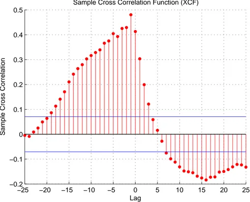
In other words, simulations shown in Figure 1 tell the following story: when a firm makes high profit, it increases its net worth. Thus, the firm wants (and has the possibility because banks evaluate it profitable) to obtain further funds from banks to enlarge its leverage. Moreover, it may have a higher target leverage: it is profitable to obtain more credit to invest in an activity with a high gain, higher than the lower cost of the credit. In good times there are the seeds of the subsequent crisis, with a possible high debt bubble. Then, in this case the pro-cyclicality of credit clearly emerges, given that during a first phase the increase of leverage (i.e., the debt grows more than proportionally than the net worth) boosts firms’ growth until the system reaches a critical point of financial fragility and the cycle is reversed through deleveraging. This feature results clearly from Figure 2: during an expansion the production growth allows to further expand the economy through increasing the leverage (negative lags in the Figure show positive correlation between firms net worth and subsequent leverage); the increase of leverage, in turn, enlarges the production (first positive lags in the Figure), but after a while the rise of financial fragility eventually leads to a recessionary phase (negative values of cross correlations’ positive lags). Indeed, when the leverage is high, this may boost production along an expansion, but the economy may also become more fragile and volatile, and then:

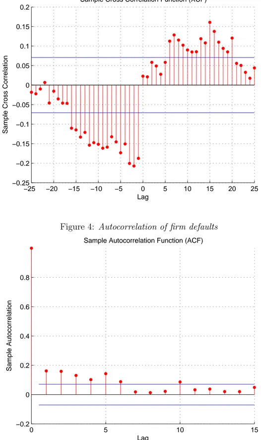
• a negative real shock for the firm can easily create a large loss when the debt is high, because there are high interests to be paid without a corresponding gain. According to what said above about the influence of the leverage on net worth (and then production), the cross-correlation function between leverage and bad debt ratio (the sum of all the debts that is not repaid by the firms defaulted in the period divided by the overall

(13)

outstanding credit) highlights the mechanism of financial fragility (Figure 3): during the expansionary phase of the cycle, the decrease of firm defaults reduces the bad debt ratio and the accumulation of capital proceeds; this allows firms to borrow more (negative cross-correlations of negative lags in Figure 3) both because they are more capitalized and because banks are financially sounder. But, after some periods the increased leverage results in a “too-high” financial fragility and an increase of default (and bad debt) follows (positive cross-correlations between leverage and subsequent bad debt ratio). Thus, with the variable leverage, the standard financial accelerator is even increased and we can call it “leveraged financial accelerator”;

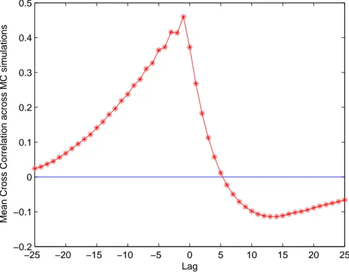
• the increased number of firms’ bankruptcies starts the “network-based accelerator”; the correlation between firm and bank defaults is clearly significant: in the same period firms and banks’ defaults are positively related, with a correlation coefficient equal to 15%. Now, the reduced bank capitalization due to the increased previous bad debt, tightens the credit supply and makes the interest rates higher for the other firms that increase the number of their defaults: this is shown by the autocorrelation function of firm defaults that shows significant positive values for some lags (see fig.4)8_.

Figure 1 shows that, in our simulations, financial fragility creates quite strong bankruptcies avalanches with the number of defaulted banks in the same period that is in mean equal to 1.28 but varies from a minimum of 0 to a maximum of 5 (the 10% of the banks in the economy); moreover, bankruptcies tend to cluster in subsequent periods; the distribution of bank defaults presents positive skewness (more than 0.7) and high kurtosis (6.15). However,

this propagation could be dampened (or increased) considering the interbank market9_{, that}

we want to introduce in further extensions of the present model.

Analyzing firm bankruptcies, we observe that they vary from a minimum of 55 (11% of overall firms) to a maximum of 105 (21%), with a mean of 77.86 and a distribution with a high kurtosis of 5.9.

8_{We can see it also in the not reported cross-correlation function between firm bankruptcies and bad debt} ratio: a higher bad debt ratio increases the following periods’ bankruptcies and, by definition, bankruptcies increase the same period bad debt.

9_{There is an increasing literature branch that is studying the ability of the interbank market in reducing} the systemic/contagion risk, since the seminal paper of Allen and Gale (2001), with works such as Acharya (2009), Allen et al. (2010); Brock et al. (2009), Castiglionesi and Navarro (2010), Gai and Kapadia (2010), Haldane and May (2011), Ibragimov et al. (2011), Ibragimov and Walden (2007), Nier et al. (2007), Shin (2008, 2009), Stiglitz (2010), Wagner (2009) and so on. Many of these papers highlight that an increasing connectivity of the interbank network implies a more severe trade-off between the stabilizing effect of risk diversification and the destabilizing effect of bankruptcy cascades.

(14)

Figure 1: Baseline model: simulation results 200 400 600 800 1000 104.5 104.6 Aggregate production 200 400 600 800 1000 0 0.01 0.02 0.03 0.04

Bad debt ratio

200 400 600 800 1000 1.8 2 2.2 2.4 2.6 Leverage 200 400 600 800 1000 0 2 4 6 Bank defaults

Figure 2: Cross-correlation between firms’ leverage and net worth

−25 −20 −15 −10 −5 0 5 10 15 20 25 −0.2 −0.1 0 0.1 0.2 0.3 0.4 0.5 Lag

Sample Cross Correlation

(15)

Figure 3: Cross-correlation between firms’ leverage and bad debt −25 −20 −15 −10 −5 0 5 10 15 20 25 −0.25 −0.2 −0.15 −0.1 −0.05 0 0.05 0.1 0.15 0.2 Lag

Sample Cross Correlation

Sample Cross Correlation Function (XCF)

Figure 4: Autocorrelation of firm defaults

0 5 10 15 −0.2 0 0.2 0.4 0.6 0.8 Lag Sample Autocorrelation

(16)

5.1 Robustness check

We implement a simple Monte Carlo experiment, repeating the simulation 100 times with different seeds of the random numbers, to check the robustness of our findings.

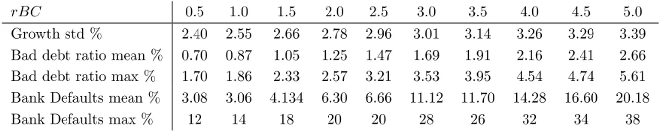
All features are confirmed (see Table 2 and compare it with Tables in the appendix). For example, we report the two cross-correlation functions between leverage and net worth or bad debt ratio, two of the most important characteristics emerging from simulations. Figures 5 and 6 confirm the cyclical behavior of leverage. Indeed, we detect a strong positive correlation between net worth and the subsequent leverage (that is negative lags in Figure 5) in all the 100 simulations, while we find a negative correlation between leverage and the following net worth (positive lags in Figure 5) in 91 cases out of 100. Moreover, we observe a strong evidence of negative correlation between bad debt ratio and the subsequent leverage (negative lags in Figure 6) in all simulations, while a positive correlation between leverage and the following bad debt (positive lags in Figure 6) emerges in 97 cases out of 100.

Table 2: Mean, minimum and maximum of relevant statistics across 100 simulations

mean min max Growth std % 3.30 3.09 3.54 Leverage mean 2.09 2.05 2.14 Leverage maximum 2.57 2.41 2.87 Bad debt ratio mean % 1.10 1.05 1.15 Bad debt ratio max % 4.33 3.07 6.74 Bank Defaults mean % 3.14 2.30 4.18 Bank Defaults max % 12.48 8 20

5.2 Sensitivity analysis

In this section we discuss the effects of model parameters’ changes (keeping all the other vari-ables fixed at the level set in Table 1) in terms of the following output varivari-ables: the volatility of the aggregate production’s growth rate, average and maximum value of overall leverage in

the economy, average and maximum value of bad debt ratio10_{, average and maximum number}

of bank defaults. In this way we check the sensitivity of our findings to the hypotheses on the parameter setting and we can observe some interesting results.

α (see Table 5). We change the mean gain from 2% to 20% with steps of 2%. The higher the average profit for firms the more stable the economic system is. Indeed, the number of firm defaults decreases (when α is 2%, 121.9 firms go bankrupt in mean every period, while when it is 20% the number of mean defaults is 35.5) and, because of the reduction of the bad debt ratio, the overall banking system is less fragile (more capitalized) and bank defaults decrease (from 36.87% to 0), with a lower and lower correlation between firm and bank defaults. The

(17)

Figure 5: Mean cross correlation between firms’ leverage and net worth −25 −20 −15 −10 −5 0 5 10 15 20 25 −0.2 −0.1 0 0.1 0.2 0.3 0.4 0.5 Lag

Mean Cross Correlation across MC simulations

Figure 6: Mean cross correlation between firms’ leverage and bad debt

−25 −20 −15 −10 −5 0 5 10 15 20 25 −0.25 −0.2 −0.15 −0.1 −0.05 0 0.05 0.1 Lag

(18)

larger capital accumulation implies a higher level of aggregate production, further enlarged by a higher debt level, also tied to the higher leverage level, due to higher expected profits. The increased stability emerges even if the system has a higher leverage, thus, a stronger economy can support a limited increase of leverage.

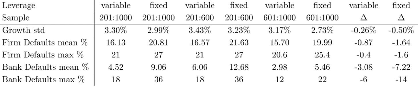
varp (see Table 6). We change the variance of the Normal random shock from 0.24 to 0.60 with steps of 0.04. We find that an increasing gain volatility implies a more volatile economy, with a growing number of firm bankruptcies (from a mean of almost 24.3 with varp 0.24, to a mean of 121.2 when varp is 0.60) and of the bad debt ratio. Then, an increase of bank defaults follows (there are almost no defaults with variance 0.24, while 27.81% of banks go bankrupt in mean every period when variance is 0.60) with a higher and higher correlation between firm and bank defaults. The effect of bankruptcy cascades is also very evident: when varp is equal to 0.6, there are periods in which the number of firm defaults reaches the 150 units and periods in which the number of bank defaults reaches the number of 26 (more than a half of the banks in the system). Moreover, leverage increases (because the biggest firms, that have very high profits, enlarge their production with higher leverage too) and it further enlarges the financial fragility and the accelerator mechanism, as shown by the cross-correlation between leverage and bad debt that is not statistically significant for low values of varp.

adj see Section 6.

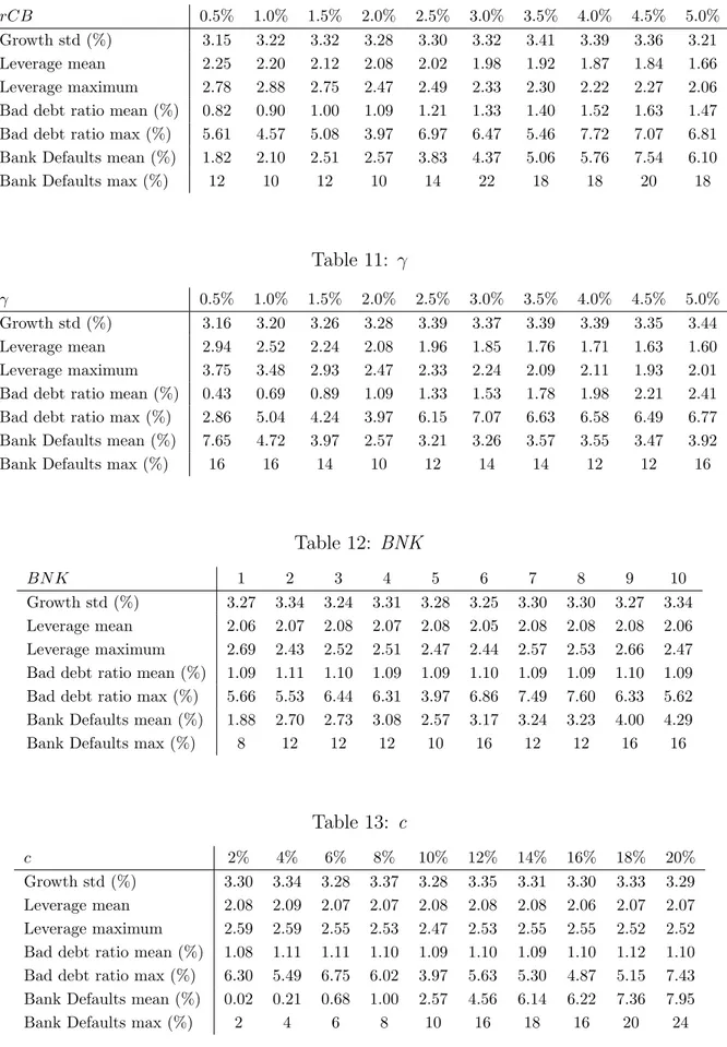
φ (see Table 8). A higher value of this parameter implies a higher volatility of aggregate production. It is worth to note that this is related to a higher level of the aggregate production itself. Then, a trade-off between production level and its volatility emerges. The leverage shows a slight increase of its mean and a larger rise of volatility/maximum. A similar pattern is followed by the bad debt ratio and, consequently, we observe an increase of bank defaults. β (see Table 9). A growth of β increases the volatility of the aggregate production’s growth rate, the leverage level, the number of defaults and the amount of the bad debt ratio. Moreover, a high β implies very strong cascade effects, with events characterized by high values of maximum leverage, bad debt ratio and bank defaults.

rCB see Section 7.

γ (see Table 11). A high γ, increasing the risk premium, increases the mean interest rate even if the leverage is reduced (due to the fact that is less convenient to borrow money at high interest rates). Then, the number of firm bankruptcies increases. However, the increased bad debt does not create problems to banks, because they earn very large profit thanks to the high interest rates on non defaulted firms.

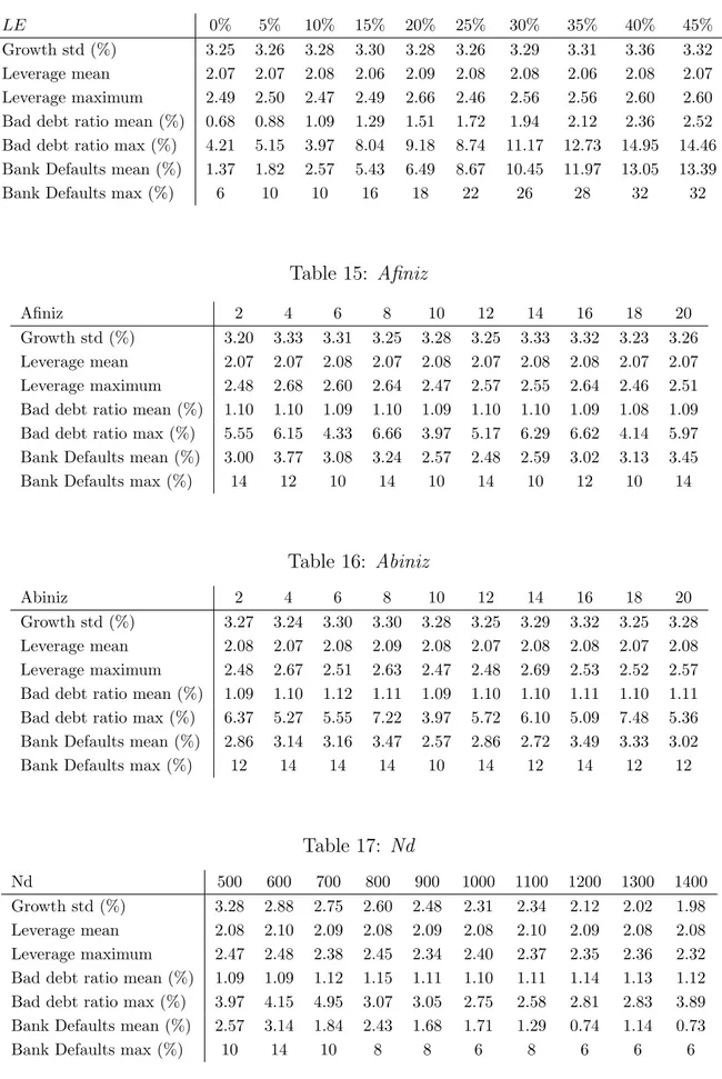
Minor parameters. The number of observed banks BN K (see Table 12) influences the number of bank defaults only, given that when firms have a larger set of banks among which to choose the best partner, they tend to concentrate on the cheapest ones, so implying the failure of minor banks. The parameter c (see Table 13) has a similar effect. A relevant in-crease of bank defaults is also caused by an inin-crease of parameter LE (see Table 14): if the

(19)

recovery rate (RR) is reduced, the amount of bad debt increases for a given number of firm defaults; then, it strongly affects bank profits and the number of bank defaults. The policy maker has to develop the laws about bankruptcies also to improve the stability of banks. The fact that bank defaults are not strongly related to other output variables, and in partic-ular to aggregate production, is the consequence of our simplifying assumption of one-to-one replacement of bankrupt agents. Indeed, in certain circumstances, for instance when BN K, c or LE are “high”, small banks tend to fail with a high probability and they are replaced by new “small” entrants that stabilize the system and, in turn, have a high probability to fail, and so on. As a consequence, the banking system becomes more concentrated and a large fraction of firms, that continues to borrow from large banks, does not have consequences from the high default rate of (small) banks. This is one of the assumptions we want to remove in our future research on the topic.

Initial conditions. Computer simulations are robust to changes in initial conditions of the firms’ net worth (Afiniz) (see Table 15) and of the banks’ net worth (Abiniz) (see Table 16). We also simulate the system for different ratios between the number of firms and banks: from 500/50 to 1400/50 adding 100 firms for each of the ten steps (keeping constant the number of banks). Simulations are again robust to this change, the only difference being a decreasing volatility of the growth rate, and a decreasing number of bank defaults given that each bank has more customers (see Table 17).

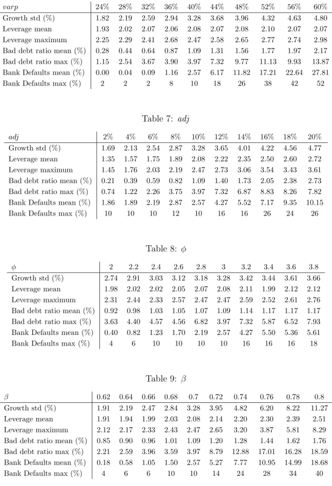
6 From variable to fixed target leverage

We devote this section to the sensitivity analysis of the parameter adj that is the most important variable regarding the leverage behavior. We change it from 2% to 20% with steps of 2%. When adj increases an increase of all output variables analyzed follows (see Table 7). In particular, a strong adjustment of the leverage level increases the volatility of the system both in terms of the aggregate production’s growth rate and failures (bad debt ratio). It is worth to note that cascades of bad debt are more likely to appear for larger values of adj (for example, when adj = 20%, the average of the bad debt ratio is around 2.7% and a cascade of more than 7.8% magnitude may happen). It clearly emerges that a higher mean leverage (due to the fact that the skewness of leverage distribution is higher when adj is higher: the distribution of the leverage has a lower bound in 0, while it has not an upper bound theoretically) and a higher pro-cyclicality of the leverage increase the “leveraged network-based financial accelerator” with a destabilizing effect on the economy. Instead, as adj decreases the pro-cyclicality of the leverage becomes less evident.

Geanakoplos (2010) finds that leverage is pro-cyclical, while Kalemli-Ozcan et al. (2011), as well as Adrian and Shin (2008,2009), find that the leverage pattern for non-financial firms is acyclical (instead this is pro-cyclical for investement banks and large commercial banks). We simulate the model also for adj even smaller than 2%, approaching zero, finding that our

(20)

model is able to reproduce also this acyclical pattern. If adj is equal to zero, the financial structure of the model changes and it is based on a fixed leverage target (that is the standard trade-off theory). In this scenario, the leverage becomes even counter-cyclical11_{. Accordingly,}

our model gives rise to different patterns of leverage along the business cycle: from pro-cyclical to acyclical and even counter-cyclical.

In Section 7 we will compare this simulation with those where the leverage target is fixed. The simulation with fixed leverage target has a smaller standard deviation of the production

growth12 _{(2.81%, as shown in Table 3, compared to 3.28% of our baseline model), because}

there is not the pro-cyclicality of the leverage that increases investments in growth periods and decreases them during recessions: do not considering the leverage pro-cyclicality makes it lose a component of volatility due to the financial accelerator.

Moreover, with a variable leverage also big firms go bankrupt, as shown by the maximum reached by the bad debt ratio that is higher than the maximum reached with fixed target leverage (3.97% vs 2.72%) even if the mean bad debt is similar and the number of firm defaults is higher when the target is fixed (in mean 77.8 vs 98.7, with a maximum of 105 vs 126). The reason is that a firm that has a high profit enlarges its net worth, but also its leverage, thus it could be financially fragile even with a high net worth.

The inverse relation between firm net worth and leverage is also the cause of another difference between the two simulations. Indeed, the number of bank defaults is higher if the leverage is fixed. The reason is that, in case of a fixed leverage target, a negative correlation between net worth and leverage emerges: a net worth reduction can pursue the real leverage over the target; in this case banks do not constraint the credit to firms, then they are more exposed. Instead, the variable leverage simulation presents, as already explained, a positive correlation between net worth and leverage; this is a better description of the credit constraint applied by banks to their borrowers during the last crisis. In this way banks reduce their risks and their probability of default, reacting to the external changes.

11_{In this case, the exogenous choice of the fixed target leverage is fundamental, while in the variable leverage} target setting the system evolves to an endogenous target, reducing the impact of the initial condition. In order to compare this simulation with the baseline simulation, we set the fixed target leverage at 2. The effective mean leverage is a bit over the target - about 2.09, very close to the mean leverage which emerges from the baseline model - and has a small, but non-null variance, because of the mechanism of equation 5 explained in section 3.1. This mechanism is also the cause of the counter-cyclical pattern: a firm facing a huge net worth loss should proportionally reduce the debt, but it could be not feasible at all if the previous period debt is so high that pushes the leverage above the target.

12_{The growth rate is calculated on firms’ production only. The banking sector component is not included} in the product computation.

(21)

7 Monetary policy experiments

In this section we first show the effect of the sensitivity analysis on rCB and then we analyze a couple of monetary policy experiments. As already said, stochastic prices fluctuate around a common mean, then the Central Bank does not follow an inflation target strategy or somewhat similar focused on the control over inflation through interest rate changes. However, we find interesting to investigate the influences of monetary policy on the financial stability of the system.

When rCB (see Table 10) increases, firms’ financial conditions weaken. This has two consequences:

• firm defaults and the bad debt ratio increase, so leading to a higher number of bank defaults;

• firms ask for less credit, reducing the leverage.

The second effect counteracts the first. Indeed, if we repeat the same sensitivity analysis (as shown in Table 3) setting the leverage target at the fixed level of 2, we find that a higher interest rate has much stronger consequences: firm and bank defaults significantly increase if compared to the simulation with floating leverage, and the growth volatility is also larger, because the system does not adapt itself to the new monetary conditions.

Then, model findings suggest that Central Bank should consider this effect of the monetary policy change on the leverage when deciding monetary policy changes. For example, a reduc-tion of the interest rate made to revitalize the economy, could increase the overall leverage and, then, the volatility of the system, with possible negative cascade effects.

Table 3: rCB with leverage target = 2

rBC 0.5 1.0 1.5 2.0 2.5 3.0 3.5 4.0 4.5 5.0

Growth std % 2.40 2.55 2.66 2.78 2.96 3.01 3.14 3.26 3.29 3.39 Bad debt ratio mean % 0.70 0.87 1.05 1.25 1.47 1.69 1.91 2.16 2.41 2.66 Bad debt ratio max % 1.70 1.86 2.33 2.57 3.21 3.53 3.95 4.54 4.74 5.61 Bank Defaults mean % 3.08 3.06 4.134 6.30 6.66 11.12 11.70 14.28 16.60 20.18

Bank Defaults max % 12 14 18 20 20 28 26 32 34 38

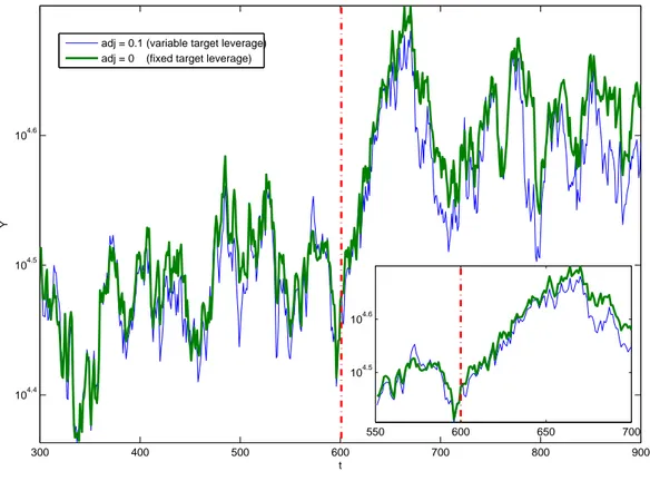
Now we analyze the following policy experiment: we modify the interest rate during the simulation to show the different impact of a monetary policy in a context of fixed vs variable leverage. When the policy rate decreases (increases) a short-run expansion (restriction) of aggregate production follows (after a while the growth rate converges to the long-run level) with a fall (growth) of firm and bank defaults: the economy passes from a steady state to another, with a period of growth (recession). Figure 7 shows the short-run expansion due to a policy rate decreases from 4% to 2% at time 600, both for a simulation with fixed leverage

(22)

(dash-dot line) and with variable leverage (solid line). We can observe that the effect of the monetary expansion is stronger in the case of fixed leverage. To confirm this finding, we report some statistics in Table 4: the last two columns show the difference between growth standard deviation, firm defaults and bank defaults before and after the interest rate change. It is evident that do not considering the influence of the monetary rate on leverage makes the central bank overestimate the strenght of the monetary policy. The reason is, as already observed, the leverage increases due to the reduction of the interest rate: when the central bank interest rate is set at 4% the mean leverage is 1.89, with a standard deviation of 9.63% and a maximum of 2.19; instead, when the central bank interest rate is set at 2% the mean leverage is 2.03, with a standard deviation of 12.32% and a maximum of 2.35; then, a higher and more volatile leverage counteracts the positive effects of the monetary expansion, making the economy relatively more fragile.

Figure 7: Monetary policy easing with variable vs. fixed target leverage

300 400 500 600 700 800 900 104.4 104.5 104.6 t Y 550 600 650 700 104.5 104.6 adj = 0.1 (variable target leverage)

adj = 0 (fixed target leverage)

We try another experiment. In this case we keep the leverage target variable and we implement a monetary tightening from 2% to 4% in two simulations with a different value of bank costs c: 2% and 10%. As already explained, the monetary tightening creates a recession phase, but after a while the growth rate converges to the long-run level. However, after the recession phase, the number of bank defaults remains higher (from 2.12% to 5.62% mean bank default per period) in the simulation where c is 10%, because the banking system is less capitalized and the increased number of firm bankruptcies makes it more fragile. On the other

(23)

Table 4: Monetary policy with variable target leverage and fixed target leverage at 2.

Leverage variable fixed variable fixed variable fixed variable fixed Sample 201:1000 201:1000 201:600 201:600 601:1000 601:1000 ∆ ∆

Growth std 3.30% 2.99% 3.43% 3.23% 3.17% 2.73% -0.26% -0.50%

Firm Defaults mean % 16.13 20.81 16.57 21.63 15.70 19.99 -0.87 -1.64

Firm Defaults max % 21 27 21 27 20.6 25.4 -0.4 -1.6

Bank Defaults mean % 4.52 9.06 6.06 12.68 2.98 5.46 -3.08 -7.22

Bank Defaults max % 18 36 18 36 12 22 -6 -14

‘Variable ∆’ represents the difference between column ‘variable 601:1000’ and column ‘variable 201:600’, while ‘fixed ∆’ represents the difference between column ‘fixed 601:1000’ and column ‘fixed 201:600’.

hand, when c is equal to 2% there is no variation between the two sub-samples (before and after the monetary restriction), given that there are almost no bank failures in both. Thus, the important policy implication is: a Central Bank that wants to increase the interest rate, should previously check if the banking system is well capitalized, to avoid cases such as the financial crises started in 2007 after a monetary restriction phase.

8 Conclusions

In this paper we build on the agent based model of Delli Gatti et al. (2010), determining the firms’ financial structure with the dynamic trade-off theory (Flannery and Rangan, 2006), adding multiperiodal debts and the loss given default rate in bankruptcies.

Following the dynamic trade-off theory, we hypothesize that firms have a target leverage. It implies that a growing firm will couple the increasing capital with increasing debt exposure, thus creating in good times the basis for the subsequent crisis. Then, we enrich the positive feedback mechanism tied to the network-based financial accelerator of Delli Gatti et al. (2010), with the pro-cyclicality of leverage. Indeed, a negative shock on firms’ output makes banks less willing to loan funds (the same holds for risk averse firms characterized by dynamic trade-off theory), hence firms might reduce their investment both because of less internal funds and because of a reduced leverage due to the increased interest rates faced (or a credit constraint) and the reduced investment leads again to lower output. Moreover, there is the network-based accelerator: bankruptcies deteriorate banks’ financial condition and this leads to higher interest rates to all borrowers (Stiglitz and Greenwald, 2003, p.145), further increasing the financial weakness of the whole non-financial sector. Thus, the presence of a credit network may produce an avalanche of firms’ bankruptcies, in another vicious circle that can make banks go bankrupt too. The last mechanism makes possible that an idiosyncratic shock creates an extended/global crisis, without the need of a systemic shock.

(24)

reproduce some of those already found in Delli Gatti et al. (2010), such as the emergent right-skew distribution of firms’ and banks’ size from firms that start with the same conditions, even without the use of trade-credit between two different kinds of firms (upstream and downstream).

As already said, the first result concerns the leverage: if it increases, the economy is riskier, with a higher volatility of aggregate production and an increase of firms and banks’ defaults. Moreover, if the leverage target is variable (positively related to gains and negatively related to interest rate), the pro-cyclicality of credit clearly emerges. During the expansionary phase of the cycle, gains make firms accumulate capital and the decrease of firm defaults reduces the bad debt; this allows firms to borrow more both because they are more capitalized and banks are financially sounder thus lending at favourable terms. However, the overall spread could be higher due to the increased leverage. The higher leverage boosts firms’ growth until the system reaches a critical point of financial fragility and the cycle is reversed through an in-crease of defaults. In this framework the network-based financial accelerator is even inin-creased and we can call it “leveraged network-based financial accelerator”.

In particular, if leverage changes rapidly (adj increases), the volatility of the system grows both in terms of the aggregate production’s growth rate and in the number of failures. Moreover, cascades of bad debt are more likely to appear for larger values of adj: a higher pro-cyclicality of the leverage increases the “leveraged network-based financial accelerator” with a destabil-izing effect on the economy.

Another result is tied to the consideration of the recovery rate (RR) or loss given default rate (LGDR). The amount of losses that banks suffer in case of borrowers’ default is a variable strongly significant in determining the number of bank defaults. Thus, an increase of the LGDR causes a growth of bank defaults and the banking system becomes more concentrated (in fact, many banks near to bankruptcy were acquired by financially sounder ones). The policy maker has to develop the laws about bankruptcies also to improve the stability of banks and, then, of the economic system.

Comparing this model to a model with fixed leverage target, some other features emerge: with variable leverage big firms go bankrupt too, because a firm that has a high profit enlarges its net worth but also its leverage, thus it could be financially fragile even with a high net worth. On the other hand, a variable leverage reduces the number of bank defaults because there is a strong credit constraint (interest rate hike) during the crisis.

The most important result regards the monetary policy. When the policy rate decreases (increases) a short-run expansion (restriction) of aggregate production follows (after a while the growth rate converges to the long-run level) with a fall (rise) of firm and bank defaults. However, the presence of a variable leverage target weakens this effect because, for example, when rCB decreases, firms ask more credit enlarging the leverage and this mechanism coun-teracts the standard expansionary effect, increasing the volatility of the system. Indeed, if we repeat the same sensitivity analysis setting the leverage target at a fixed level, we find

(25)

that monetary policy change has much stronger consequences. Thus, the incorporation of the effect of the interest rate on the leverage exposure of firms should be considered by the Central Bank when deciding monetary policy changes.

The last result concerns again the monetary policy. A monetary tightening creates a re-cession phase, but it also creates a higher number of bank failures when the banking system is poorly capitalized. Then, a Central Banks that wants to increase the interest rate, should previously check if the banking system is well capitalized, to avoid cases such as the financial crises started in 2007 after a monetary restriction phase. In future works it would be inter-esting to see whether the same holds when an increase of the reserve requirements is decided or the Central Bank may follow this alternative way to implement a monetary tightening considering banks’ financial solidity. Moreover, in order to improve the analysis of monetary policy, we are going to extend our framework to also consider the role of the Central Bank in stabilizing the financial system through ’monetary easing’ measures, even when interest rates are close to zero.

References

[1] Acharya V.V. (2009), “A theory of systemic risk and design of prudential bank regula-tion”, Journal of Financial Stability, 5(3): 224-255.

[2] Adrian, T., Shin, H.S. (2008) “Liquidity, monetary policy and financial cycles”, Current

Issues in Economics and Finance, 14(1), Federal Reserve Bank of New York (Janu-ary/February).

[3] Adrian, T., Shin, H.S. (2009), “Money, Liquidity, and Monetary Policy”, American

Eco-nomic Review, 99(2): 600-605.

[4] Adrian, T., Shin, H.S. (2010), “Liquidity and leverage”, Journal of Financial

Intermedi-ation, 19(3): 418-437.

[5] Allen F., Babus A., Carletti E. (2010), “Financial Connections and Systemic Risk”,

NBER Working Papers 16177.

[6] Allen F., Gale D. (2001), “Financial contagion”, Journal of Political Economy, 108: 1-33. [7] Baker M., Wurgler J. (2002), “Market timing and capital structure”, The Journal of

Finance, 57: 1-32.

[8] Brunnermeier M.K., Pedersen L.H. (2009), “Market liquidity and funding liquidity”,

Review of Financial Studies, 22(6): 2201-2238.

[9] Bernanke B., Gertler M. (1989) “Agency costs, net worth and business fluctuations”,

(26)

[10] Bernanke B., Gertler M. (1990), “Financial fragility and economic performance”,

Quarterly Journal of Economics, 105: 87-114.

[11] Bernanke B., Gertler M., Gilchrist S. (1999), “The financial accelerator in a quantitative business cycle framework”, in: Taylor J., Woodford M. (Eds.), Handbook of

Macroeco-nomics, Vol. 1, North Holland, Amsterdam, 1341-1393.

[12] Booth L., Asli Demirgu-Kunt V.A., Maksimovic V. (2001), “Capital Structures in De-veloping Countries”, Journal of Finance, 56(1): 87-130.

[13] Brock W.A., Hommes C.H., Wagener F.O.O. (2009), “More hedging instruments may destabilize markets”, Journal of Economic Dynamics and Control, 33(11): 1912-1928. [14] Castiglionesi F., Navarro N. (2010), “Capital Fragile Financial Networks”, Tilburg

Uni-versity, mimeo.

[15] Delli Gatti D., Gallegati M., Greenwald B., Russo A., Stiglitz J.E. (2010), “The financial accelerator in an evolving credit network”, Journal of Economic Dynamics and Control, 34(9): 1627-1650.

[16] Diamond D.W., Rajan R. (2000), “A Theory of Bank Capital”, Journal of Finance, 55(6): 2431-2465.

[17] Donaldson G. (1961), “Corporate debt capacity: a study of corporate debt policy and the determination of corporate debt capacity”, Harvard Business School, Harvard University. [18] Flannery M.J. (1994), “Debt Maturity and the Deadweight Cost of Leverage: Optimally

Financing Banking Firms”, American Economic Review, 84(1): 320-31.

[19] Flannery M.J., Rangan K.P. (2006), “Partial adjustment toward target capital struc-tures”, Journal of Financial Economics, 79(3): 469-506.

[20] Fostel A., Geanakoplos J. (2008), “Leverage Cycles and the Anxious Economy”,

Amer-ican Economic Review, 98(4): 1211-44.

[21] Frank M.Z., Goyal V.K. (2008), “Tradeoff and Pecking Order Theories of Debt”, in: Espen Eckbo (ed.) The Handbook of Empirical Corporate Finance, Ch. 12: 135-197. [22] Gai P., Kapadia S. (2010), “Contagion in financial networks”, Proceedings of the Royal

Society A, 466: 2401-2423.

[23] Geanakoplos J. (2010), “Leverage cycle”, Cowles foundation Paper No. 1304, Yale Uni-versity.

(27)

[24] Graham J.R., Harvey C. (2001), “The Theory and Practice of Corporate Finance”,

Journal of Financial Economics, 60: 187-243.

[25] Greenlaw D., Hatzius J., Kashyap A.K., Shin H.S. (2008), “Leveraged Losses: Lessons from the Mortgage Market Meltdown”, Proceedings of the U.S. Monetary Policy Forum. [26] Greenwald, B., Stiglitz, J.E. (1993), “Financial market imperfections and business

cycles”, Quarterly Journal of Economics, 108: 77-114.

[27] Gropp R., Heider F. (2010), “The Determinants of Bank Capital Structure”, Review of

Finance, 14(4): 587-622.

[28] Haldane A.G., May R.M. (2011), “Systemic risk in banking ecosystems ”, Nature, 469: 351-355.

[29] He Z., Khang I.G., Krishnamurthy A. (2010), “Balance Sheet Adjustments in the 2008 Crisis”, IMF Economic Review, 58: 118-156.

[30] Hovakimian A., Opler T., Titman S. (2001), “The Debt-Equity Choice”, Journal of

Financial and Quantitative Analysis, 36: 1-24.

[31] Ibragimov R., Walden J. (2007), “The limits of diversification when losses may be large”,

Journal of Banking and Finance, 31: 2551-2569.

[32] Ibragimov R., Jaffee D., Walden J. (2011), “Diversification disasters”, Journal of financial

Economics, 99: 333-348.

[33] Jensen M.C., Meckling W.H. (1976), “Theory of the Firm: Managerial Behavior, Agency Costs, and Ownership Structure”, Journal of Financial Economics, 3: 305-360.

[34] Kalemli-Ozcan S., Sorensen B., Yesiltas S. (2011), “Leverage Across Firms, Banks, and Countries”, NBER Working Papers 17354.

[35] Lemmon M., Roberts M., Zender J. (2008), “Back to the beginning: Persistence and the cross-section of corporate capital structure”, Journal of Finance, 63: 1575-1608.

[36] Mehrotra V., Mikkelsen W., Partch M. (2003), “Design of Financial Policies in Corporate Spinoffs”, Review of Financial Studies, 16: 1359-1388.

[37] Myers, S.C. (1977), “Determinants of corporate borrowing”, Journal of Financial

Eco-nomics, 5(2): 147-175

[38] Myers, S.C., Majluf N.S. (1984), “Corporate Financing and Investment Decisions When Firms Have Information that Investors Do Not Have”, Journal of Financial Economics, 13: 87-224.

(28)

[39] Nier E., Yang J., Yorulmazer T., Alentorn, A. (2007), “Network Models and Financial Stability”, Journal of Economic Dynamics and Control, 31(6): 2033-2060.

[40] Rajan R., Zingales L. (1995), “What do we know about capital structure? Some evidence from international data”, Journal of Finance, 50: 1421-1460.

[41] Shin, H. (2008), “Risk and Liquidity in a System Context”, Journal of Financial

Inter-mediation, 17: 315-329.

[42] Shin, H.S. (2009), “Securitisation and Financial Stability”, Economic Journal, 119: 309-332.

[43] Stiglitz J.E. (2010), “Risk and Global Economic Architecture: Why Full Financial In-tegration May Be Undesirable”, American Economic Review, 100(2): 388-92.

[44] Stiglitz J.E., Greenwald B. (2003), Towards a New Paradigm in Monetary Economics, Cambridge University Press, Cambridge.

[45] Wagner W. (2009), “Efficient Asset Allocations in the Banking Sector and Financial Regulation”, International Journal of Central Banking 5(1): 75-95.

A

Sensitivity Analysis: Tables

Table 5: α

α 2% 4% 6% 8% 10% 12% 14% 16% 18% 20%

Growth std (%) 4.01 3.83 3.81 3.52 3.28 3.09 2.77 2.62 2.52 2.40 Leverage mean 1.55 1.64 1.86 1.95 2.08 2.20 2.32 2.43 2.55 2.67 Leverage maximum 2.48 2.20 2.65 2.37 2.47 2.67 2.73 2.70 2.87 2.97 Bad debt ratio mean (%) 3.37 2.36 1.97 1.44 1.09 0.89 0.73 0.63 0.58 0.54 Bad debt ratio max (%) 11.86 9.89 6.14 6.90 3.97 4.67 4.48 3.37 2.87 2.63 Bank Defaults mean (%) 36.87 25.45 17.73 8.74 2.57 0.96 0.15 0.02 0.00 0

(29)

Table 6: varp

varp 24% 28% 32% 36% 40% 44% 48% 52% 56% 60%

Growth std (%) 1.82 2.19 2.59 2.94 3.28 3.68 3.96 4.32 4.63 4.80 Leverage mean 1.93 2.02 2.07 2.06 2.08 2.07 2.08 2.10 2.07 2.07 Leverage maximum 2.25 2.29 2.41 2.68 2.47 2.58 2.65 2.77 2.74 2.98 Bad debt ratio mean (%) 0.28 0.44 0.64 0.87 1.09 1.31 1.56 1.77 1.97 2.17 Bad debt ratio max (%) 1.15 2.54 3.67 3.90 3.97 7.32 9.77 11.13 9.93 13.87 Bank Defaults mean (%) 0.00 0.04 0.09 1.16 2.57 6.17 11.82 17.21 22.64 27.81

Bank Defaults max (%) 2 2 2 8 10 18 26 38 42 52

Table 7: adj

adj 2% 4% 6% 8% 10% 12% 14% 16% 18% 20%

Table 8: φ

φ 2 2.2 2.4 2.6 2.8 3 3.2 3.4 3.6 3.8

Table 9: β

β 0.62 0.64 0.66 0.68 0.7 0.72 0.74 0.76 0.78 0.8

(30)

Table 10: rCB

rCB 0.5% 1.0% 1.5% 2.0% 2.5% 3.0% 3.5% 4.0% 4.5% 5.0%

Table 11: γ

γ 0.5% 1.0% 1.5% 2.0% 2.5% 3.0% 3.5% 4.0% 4.5% 5.0%