Received January 15, 2013 Published as Economics Discussion Paper January 29, 2013 Revised July 21, 2013 Accepted October 29, 2013 Published November 25, 2013
Unemployment Benefits and Financial Leverage in
an Agent Based Macroeconomic Model
Luca Riccetti, Alberto Russo, and Mauro Gallegati
Abstract
This paper is aimed at investigating the effects of government intervention through unemployment benefits on macroeconomic dynamics in an agent based decentralized matching framework. The major result is that the presence of such a public intervention in the economy stabilizes the aggregate demand and the financial conditions of the system at the cost of a modest increase of both the inflation rate and the ratio between public deficit and nominal GDP. The successful action of the public sector is sustained by the central bank which is committed to buy outstanding government securities.
Published in Special Issue Economic Perspectives Challenging Financialization, Inequality and Crises
JEL E32 C63
Keywords Agent based macroeconomics; business cycle; crisis; unemployment; leverage Authors
Luca Riccetti, Sapienza Università di Roma, Department of Management,
Alberto Russo, Università Politecnica delle Marche, Department of Economics and Social
Sciences, Piazzale Martelli 8, 60121 Ancona, Italy, [email protected]
Mauro Gallegati, Università Politecnica delle Marche, Department of Economics and Social
Sciences, [email protected]
Citation Luca Riccetti, Alberto Russo, and Mauro Gallegati (2013). Unemployment Benefits and Financial Leverage in an Agent Based Macroeconomic Model. Economics: The Open-Access, Open-Assessment E-Journal, Vol. 7, 2013-42. http://dx.doi.org/10.5018/economics-ejournal.ja.2013-42
1 Introduction
In this paper we explore the effects of government intervention through unem-ployment benefits on macroeconomic dynamics. In particular, we slightly modify the agent based decentralized matching macroeconomic model proposed in Ric-cetti et al. (2012) to allow the government to transfer a certain amount of money to unemployed people. In general, we show that the presence of such a public intervention in the economy stabilizes the aggregate demand and the financial conditions of the system at the cost of a modest increase of both the inflation rate and the ratio between public deficit and nominal GDP. The successful action of the public sector is sustained by the operation of the central bank which is committed to buy outstanding government securities.
There is a huge literature which analyzes the role of unemployment insurance on both individual behavior and aggregate dynamics. From a microeconomic point of view, many papers analyze the nature of incentives and how the introduction of an unemployment insurance scheme modifies individual behavior regarding labor supply, that is the choice between leisure and working time. A typical result is that there is an adverse income effect of “high” unemployment insurance on the incentive to search and accept an employment opportunity. Moreover, “high” unemployment benefits reduce the opportunity costs of unemployment, resulting in a higher wage demand and an incentive to lower labor effort on the workplace. Other researchers noticed that unemployment benefits can have also positive consequences as the improvement of the quality of the matching between employers and employees (Acemoglu and Shimer, 2000) or the welfare-improving effect which emerges when people looking for jobs are liquidity constrained (Bender et al., 2009). Many contributions analyzed the effects of unemployment benefits on employment and unemployment dynamics on the basis of a “search and matching” framework (Mortensen and Pissarides, 1999a,b; Pissarides, 2000). According to this theoretical framework the presence of unemployment insurance produces more unemployment, because of the increase of workers’ bargaining power that decreases the marginal benefit for firms of the search and matching process. Moreover, the unemployment insurance operates as a friction in the labor market, modelled as a search and matching aggregate function, which amplifies business fluctuations.
In mainstream macroeconomics, the presence of unemployment benefits en-hances the bargaining power of workers with respect to firms, so leading to an increase of requested wages that, for a given mark-up set by firms, makes the “natural” rate of unemployment (Friedman, 1968; Phelps, 1968), that is the Non-Accelerating Inflation Rate of Unemployment, to rise (Turner et al., 2001). Hence, ceteris paribus, the higher the level of unemployment benefits the larger the rate of unemployment in the macroeconomic equilibrium. Basically, the “natural” rate of unemployment depends on the workers’ reservation wage (that is the bargain-ing power which is inversely dependent on the unemployment rate and directly related to the degree of unionization, unemployment benefits, etc.), the degree of monopoly in markets (that is the mark-up set by firms), and labor productivity (which depends on many variables as the accumulation of physical and human capital, and then technological progress and workers’ skills). In such a mainstream framework, there is not an impact of the aggregate demand on equilibrium unem-ployment (but for a limited period of time if agents are characterized by adaptive expectations instead of rational expectations). Accordingly, the main effect of the unemployment insurance is to act as a rigidity that pushes away the economy from Pareto optimality (the same holds for other frictions). In principle, indeed, if a demand shock hits the macroeconomy, so leading to higher unemployment, the system is able to spontaneously returns to its “natural” equilibrium through a decrease of nominal wages and (with a constant mark-up) a proportional reduction of prices (although policy makers can avoid such a deflationary process of adjust-ment through an expansionary monetary and/or fiscal policy). Moreover, in such a “natural” equilibrium setting, monetary policy is mainly addressed to assure a low and stable rate of inflation, as the best way to promote macroeconomic stability and a growth-enhancing environment (Allsopp and Vines, 2000). For these reasons, according to the conventional view, the central bank has to be independent of the government in setting monetary policy (Walsh, 2010).
However, there are many contributions in the macroeconomic field which investigate the role of unemployment insurance in stabilizing output fluctuation. The transfer of a benefit from the government to unemployed people works as an automatic stabilizer, thus providing a countercyclical action of the public sector which sustains the aggregate demand. When the credit market is imperfect, given that the relationship between lenders and borrowers is characterized by asymmetric
information (Stiglitz and Weiss, 1981), the additional liquidity provided by the government, that issues bonds to finance unemployment benefits, mitigates the credit constraint to the economy. In such an asymmetric information context, the typical working of credit markets produces financially constrained business cycles (Greenwald and Stiglitz, 1993). Consequently, the removal or at least the mitigation of the liquidity constraint may improve macroeconomic performances.
Challe et al. (2011) analyze the role of unemployment insurance when capital markets are imperfect, highliting the macroeconomic nexus between unemploy-ment benefits, public debt and liquidity-constrained firms. Their starting point is the idea that firms can mitigate the liquidity constraint through buying and holding liquid assets to be sold when they need to finance hiring and production (Holm-strom and Tirole, 1998). As a matter of fact, when firms are liquidity constrained, a higher public debt “increases the flexibility of the private sector in responding to variations in both income and spending opportunities, and so can increase economic efficiency” (Woodford, 1990, p. 382). According to Challe et al. (2011), the gov-ernment raises public debt during recessions to transfer benefits to the unemployed, thus implying an increase of liquidity supply that relaxes the credit constraint faced by firms; in this way, the government (which does not follow a balanced public budget rule) dampens the fall of employment which happens during recessions and stimulates households’ consumptions because (i) unemployed people now have an income to be spent, and (ii) the sustained aggregate demand improves firms’ profits, thus allowing for higher consumption on the part of entrepreneurs too.
As suggested by the cited literature, then, issuing public securities the govern-ment improves liquidity conditions on private markets, so mitigating the credit constraint to firms and improving macroeconomic performance. As we will see, indeed, in our model the introduction of unemployment benefits modifies the finan-cial conditions of the macroeconomy, for example influencing firms’ leverage and banks’ exposure and the impact of these financial variables on the business cycle. The recent financial turmoil has stressed the relevance of financial factors and the fundamental role of leverage cycles in shaping macroeconomic dynamics. Accord-ingly, many recent contributions have proposed an analysis of the leverage process both for firms and banks: Adrian and Shin (2008, 2009, 2010), Brunnermeier and Pedersen (2009), Flannery (1994), Fostel and Geanakoplos (2008), Greenlaw et al. (2008), He et al. (2010), Kalemli-Ozcan et al. (2011). The behaviour of the
leverage level is a component of a more general discussion on firm and bank capital structure, such as in Booth et al. (2001), Diamond and Rajan (2000), Gropp and Heider (2010), Lemmon et al. (2008), Rajan and Zingales (1995).
As for the capital structure of firms, almost all previous papers proposing an agent based approach assumed a “pecking order” theory (Donaldson, 1961; Myers and Majluf, 1984), according to which, when information is asymmetric, investments are financed first with internal funds, then with debt (if internal funds are not enough), and equity is used as a last resort. A different perspective on the firms’ financial structure was proposed by the “trade-off” theory, firstly observed in a paper concerning asset substitution (Jensen and Meckling, 1976), and in a work on underinvestment (Myers, 1977). This theory is based on the trade-off between the costs and benefits of debt and implies that firms select a target debt-equity ratio. The empirical literature found at first contrasting evidence to support these theories. Then, a refined version of the off theory was proposed: the “dynamic trade-off theory” (Flannery and Rangan, 2006). In this theory firms actively pursue target debt ratios even though market frictions temper the speed of adjustment. In other words, firms have long-run leverage targets, but they do not immediately reach them, instead they adjust to them during some periods. Dynamic trade-off seems to be able to overcome some puzzles related to the other theories, explaining the stylized facts emerged from the empirical analysis and numerous papers conclude that it dominates alternative hypotheses: Hovakimian et al. (2001), Graham and Harvey (2001), Mehotra et al. (2003), Flannery and Rangan (2006), Frank and Goyal (2008).
In this paper we implement an agent based model in which firms’ capital structure is based on the Dynamic Trade-Off theory. According to this theory, we assume that firms have a “target leverage”, that is a desired ratio between debt and net worth, and they try to reach it by following an adaptive rule governing credit demand. This capital structure is already investigated in the agent based model proposed by Riccetti et al. (2013) that builds upon the previous work by Delli Gatti et al. (2010), which was based on a firms’ capital structure given by the Pecking Order theory.
The modeling framework in which we analyze the effects of introducing unemployment benefits on financial and macroeconomic conditions is the one proposed in Riccetti et al. (2012) according to which the macroeconomy is a
complex systempopulated by heterogeneous agents (households, firms and banks) which directly interact in different markets (goods, labor, credit, and bank deposits). Then, there are two policy makers: the government and the central bank. In this context, aggregate regularities emerge from the “bottom up” (Epstein and Axtell, 1996) as statistical properties at the meso and macro levels that derive from the (simple and adaptive) individual behavioural rules and the interaction mechanisms which describe the working of markets (Tesfatsion and Judd, 2006; LeBaron and Tesfatsion, 2008).
Many papers in the field of agent based computational economics investigated the role of interaction in a heterogeneous agents setting, exploring the properties of a methodological alternative to neoclassical, that is Walrasian, microfoundation. Indeed, when we consider that the economy is a complex system in which aggre-gate regularities (from meso to macro) emerge from the decentralized interaction of a multitude of autonomous agents, Heterogeneous Interacting Agents (HIA) constitutes an effective alternative to the Representative Agent (RA) hypothesis, which is instead the typical assumption made by mainstream macroeconomics (Stiglitz and Gallegati, 2011). Various authors proposed an agent based approach to the study of complex (macro)economic dynamics; just to make a few exam-ples: Ashraf et al. (2013), Delli Gatti et al. (2005a, 2009, 2010), Deissenberg et al. (2008), Dosi et al. (2006, 2010, 2012), Fagiolo et al. (2004), Haber (2008), Howitt and Clower (2000), Lengnick (2013). On these methodological bases, some contributions have proposed an analysis of economic policy issues as the role of monetary policy (Delli Gatti et al. 2005b; Cincotti et al. 2010, 2012), fiscal policy and its effect on R&D dynamics (Russo et al., 2007), the combination of Keynesian management of aggregate demand and Schumpeterian policies aimed at promoting technological progress (Dosi et al., 2010), the interplay between income distribution and economic policies (Dosi et al., 2012), monetary and fiscal policies (Haber, 2008), the effectiveness of various stabilization policies (Westerhoff and Franke, 2012), labor market policies (Neugart, 2008), the role of regulatory policies on financial markets (Westerhoff, 2008), the effects of introducing a Tobin-like tax (Westerhoff and Dieci, 2006; Mannaro et al. 2008;), and so on. Hence, agent based models represent an alternative formulation of microfoundations suited for a complex macroeconomic system and this different approach may have important
implications for policy advice (Dawid and Neugart, 2011). For a comprehensive review, see Fagiolo and Roventini (2009, 2012).
With the present paper we add some results to the analysis of policy issues in an agent based macroeconomic framework. In particular, we show that the countercyclical intervention of the government stabilizes the aggregate demand and the resulting increase of the labor share, due to the introduction of unemployment benefits, does not damage the economic system (in term of firms’ profitability) if the benefit paid to unemployed workers is within a certain range. Instead, when unemployment benefits goes beyond a “reasonable” level, the subsequent profit squeeze leads to a marked decrease of the labor demand, resulting in a large unemployment rate and then in a fall of aggregate demand, so amplifying the recessionary phase.
The paper is organized as follows. Section 2 presents the model setup and the characteristics of the four markets which composes our economy: credit (Subsection 2.1), labor (Subsection 2.2), goods (Subsection 2.3), and bank deposits (Subsection 2.4); the evolution of agents’ wealth is described in Subsection 2.5, while the behavior of policy makers is discussed in Subsection 2.6. Model dynamics are studied in Section 3 in which we report the results of the simulation of the baseline model; we also provide some Monte Carlo experiments in order to analyze the interplay between financial and real factors, the characteristics of the business cycle and the behaviour of the system when an extended crisis happens. Then we provide a comparison of the baseline model with simulations performed in presence of unemployment benefits, highliting the potential positive effect of government intervention. In Section 5 we provide some concluding remarks.
2 The Model
Starting from Riccetti et al. (2012), we consider a macroeconomy composed of households (h = 1, 2, ..., H), firms ( f = 1, 2, ..., F), banks (b = 1, 2, ..., B), a central bank, and the government, which interact over a time span t = 1, 2, ..., T in the following four markets: (i) credit market; (ii) labor market; (iii) goods market; (iv) deposit market.
Agents are boundedly rational and follow (relatively) simple rules of behaviour in an incomplete and asymmetric information context: households try to buy con-sumption goods from the cheapest supplier; firms try to accumulate profits by selling their products to households (they set the price according to their individual excess demand) and hiring cheapest workers; workers update the asked wage according to their occupational status (upward if employed, downward if unem-ployed); households’ saving goes into bank deposits; given Basilea-like regulatory constraints, banks extend credit to finance firms’ production; firms choose the banks offering lowest interest rates, while households deposit money in the banks offering the highest interest rates. The government hires public workers, taxes private agents and issues public debt. Finally, the central bank provides money to banks and to the government given their requirements.
To go into details, in each period, at first firms and banks interact in the credit market. Firms ask for credit to banks given the demand deriving from their net worth and leverage target; the leverage level changes according to expected profits and inventories. Banks set their credit supply depending on their net worth, deposits and the quantity of money provided by the central bank. As said above, they must comply with some regulatory constraints.
Then, government, firms and households interact in the labor market. The govern-ment hires public workers. Afterwards, firms hire workers: labor demand depends on available funds, that is net worth and bank credit.
Subsequently, households and firms interact in the goods market. Firms produce consumption goods on the basis of hired workers. They put in the goods market their current period production and previous period inventories. Households decide their desired consumption on the basis of their disposable income and wealth. Finally, households determine their savings to be deposited in banks: banks and households interact in the deposit market.
The interaction between the demand and the supply sides of the four markets is set by the following decentralized matching protocol. In general, each agent in the demand side observes a list of potential counterparts in the supply side and chooses the most suitable partner according to some market-specific criteria. At the beginning, a random list of agents in the demand side – firms in the credit market, firms in the labor market, households in the goods market, and banks in the deposit market – is set. Then, the first agent in the list observes a random subset
of potential partners; this subset represents a fraction 0 < χ ≤ 1 (which proxies the degree of imperfect information) of the whole set of potential partners; thus, the agent chooses the cheapest one. For example, in the labor market, the first firm on the list, say firm f1 observes the asked wage of a subsample of workers and
chooses the agent asking for the lowest one, say worker h1.
After that, the second agent on the list performs the same activity on a new random subset of the updated potential partner list. In the case of the labor market, the new list of potential workers to be hired no longer contains the worker h1. The process
iterates till the end of the demand side list (in our example, all the firms enter the matching process and have the possibility to employ one worker).
Then, a new random list of agents in the demand side is set and the whole matching mechanism goes on until either one side of the market (demand or supply) is empty or no further matchings are feasible because the highest bid (for example, the money till available to the richest firm) is lower than the lowest ask (for example, the lowest wage asked by till unemployed workers).
As for the entry-exit process, new entrants replace bankrupted agents according to a one-to-one replacement. New agents enter the system with initial conditions we will define below. Moreover, the money needed to finance entrants is subtract from households’ wealth.1
Now, we propose a detailed description of the markets. 2.1 Credit Market
Firms aim at financing production and banks may provide credit to this end. Firm’s f credit demand at time t depends on its net worth Af t and the leverage target lf t.
Hence, required credit is:
Bdf t= Af t· lf t (1)
1 In the extreme case in which private wealth is not enough, then government intervenes. However, we can anticipate that it never happens in our simulations.
The evolution of the leverage target depends on the following rule: lf t=
lf t−1· (1 + α ·U(0, 1)) , if πf t−1/(Af t−1+ Bf t−1) > if t−1and ˆyf t−1< ψ · yf t−1
lf t−1, if πf t−1/(Af t−1+ Bf t−1) = if t−1and ˆyf t−1< ψ · yf t−1
lf t−1· (1 − α ·U(0, 1)) , if πf t−1/(Af t−1+ Bf t−1) < if t−1or ˆyf t−1≥ ψ · yf t−1
(2)
where α > 0 is a parameter representing the maximum percentage change of the relevant variable (in this case the target leverage), U (0, 1) is a random number picked from a uniform distribution in the interval (0,1), πf t−1is the gross
profit (realized in the previous period), Bf t−1is the previous period effective debt,
πf t−1/(Af t−1+ Bf t−1) is the return on assets that we will call also profit rate, if t−1
is the nominal interest rate paid on previous debts2, ˆyf t−1 represents inventories
(that is, unsold goods), 0 ≤ ψ ≤ 1 is a parameter representing a threshold for inventories based on previous period production yf t−1. Equation 2 means that the
leverage target increases (decreases) if the profit rate is higher (lower) than average interest rate and there is a low (high) level of inventories.
On the supply side, bank b offers a total amount of money Bdbt depending on net worth Abt, deposits Dbt, central bank credit mbt, and some legal constraints
(proxied by the parameters γ1> 0 and 0 ≤ γ2≤ 1 that represents respectively the
maximum admissible leverage and maximum percentage of equity to be invested in lending activities):
Bdbt= min(ˆkbt, ¯kbt) (3)
where ˆk = γ1· Abt, ¯k = γ2· Abt+ Dbt−1+ mbt. Moreover, in order to reduce risk
concentration, banks lend to a single firm up to a maximum fraction β of the total amount of the credit Bdbt. This behavioural parameter can be also interpreted as a regulatory constraint to avoid excessive concentration.
Bank b charges an interest rate on the firm f at time t according to the following equation:
ib f t = iCBt+ ˆibt+ ¯if t (4)
where iCBtis the nominal interest rate set by the central bank at time t, ˆibt is a
bank-specific component, and ¯if t = ρlf t/100 is a firm-specific component, that is
a risk premium on firm target leverage (with ρ > 0). The bank-specific component evolves as follows:
ˆibt =
( ˆibt−1· (1 − α ·U(0, 1)) , if ˆBbt−1> 0
ˆibt−1· (1 + α ·U(0, 1)) , if ˆBbt−1= 0
(5) where ˆBbt−1is the amount of money that the bank did not manage to lend to firms in the previous period.
As a result of the interaction based on the matching mechanism explained above, each firm ends up with a credit Bf t≤ Bdf t and each bank lends to firms an
amount Bbt ≤ Bdbt. The difference between desired and effective credit is equal to
Bdf t− Bf t= ˆBf t and Bdbt− Bbt= ˆBbt, for firms and banks respectively. Moreover,
we assume that banks ask for an investment in government securities equal to Γdbt= ¯kbt− Bbt. If the sum of desired government bonds exceeds the amount of
outstanding public debt then the effective investment Γbt is rescaled according to a
factor Γd bt/ ∑ Γ
d
bt. Instead, if public debt exceeds the banks’ desired demand, then
the central bank buys the residual amount. 2.2 Labor Market
First of all, the government hires a fraction g of households. The remaining part is available for working in the firms. Firm’s f labor demand depends on the total capital available: Af t+ Bf t. Each worker posts a wage wht which is updated as
follows:
wht=
(
wht−1· (1 + α ·U(0, 1)) , if h employed at time t − 1
The required wage has a minimum equal to: θ ˆpt−1(1 + τ), where θ is a positive
parameter, ˆpis the maximum price of a single good, and τ is the tax rate on labor income. This means that a worker asks at least a wage net of taxes able to buy a multiple θ of a good.
As a result of the decentralized matching between labor supply and demand, each firm ends up with a number of workers nf t and a residual cash (insufficient
to hire an additional worker). Obviously, a fraction of households may remain unemployed. In the baseline model, the wage of unemployed people is set equal to zero.
Then, we remove this assumption by introducing an unemployment benefit paid by the government. Accordingly, if the h-th worker is unemployed at time t then her income is given by:
wht= η ˆpt−1 (7)
where η is a positive parameter and ˆpis the maximum price of a single good, in order to have an unemployment benefit tied to the price level. We will explore the role of this parameter on model behavior in the computational experiments proposed below.
2.3 Goods Market
In the goods market households represent the demand side, while firms are the supply side. Households set the desired consumption as follows:
cdht= c1· wht+ c2· Aht (8)
where 0 < c1≤ 1 is the propensity to consume current income, 0 ≤ c2≤ 1 is
the propensity to consume the wealth Aht. If the amount cdht is smaller than the
average price of one good ¯p then cdht = min( ¯p, wht+ Aht). By summing up the
individual consumption of households we obtain the aggregate demand. It is worth noticing that current income derives from both a cyclical private industrial sector and an acyclical public service sector.
The amount of goods produced by the f -th firm is given by:
yf t= φ · nf t (9)
where φ ≥ 1 is a productivity parameter and nf t is the number of workers
employed by firm f at time t.
Then, firms want to sell this produced output plus the inventories ˆyf t−1. The selling price is set as follows:
pf t=
(
pf t−1· (1 + α ·U(0, 1)) , if ˆyf t−1= 0 and yf t−1> 0
pf t−1· (1 − α ·U(0, 1)) , if ˆyf t−1> 0 or yf t−1= 0
(10)
Hence, the firm rises the price if there are no inventories (and it produced some goods in the previous period) and viceversa. The minimum price at which firms want to sell their output is set such that it is at least equal to the average cost of production, that is ex-ante profits are at worst equal to zero.
As a consequence of the interaction between the supply and demand sides in the goods market, each household ends up with a residual cash, that is not enough to buy an additional good and that she will try to deposit in a bank; at the same time, firms sell an amount 0 ≤ ¯yf t ≤ yf t and they may remain with unsold
goods; as a consequence, in the next period the firm will try to sell the inventories ˆ
yf t= yf t− ¯yf t.
2.4 Deposit Market
Banks represent the demand side of the deposit market (given that they require capital to extend credit) and households are on the supply side. Banks offer an interest rate on deposits according to their funds requirement:
iDbt = ( iDbt−1· (1 − α ·U(0, 1)) , if ¯kbt− Bbt− Γbt > 0 min{iD bt−1· (1 + α ·U(0, 1)) , iCBt}, if ¯kbt− Bbt− Γbt = 0 (11)
where Γbt is the amount of public debt bought by bank b at time t. Hence,
the previous equation states that if a bank exhausts the credit supply by lending to private firms or government then it decides to increase the interest rate paid on deposits, so to attract new depositors, and viceversa. However, the interest rate on deposits can increase till a maximum given by the policy rate rCBtwhich is both
the rate at which banks could refinance from the central bank and the rate paid by the government on public bonds.
Then, households set the minimum interest rate they want to obtain on bank deposits as follows: iDht = ( iDht−1· (1 − α ·U(0, 1)) , if Dht−1= 0 iDht−1· (1 + α ·U(0, 1)) , if Dht−1> 0 (12) where Dht−1is the household h’s deposit in the previous period. This means
that a household that found a bank paying an interest rate higher or equal to the desired one decides to ask for a higher remuneration. In the opposite case, she did not find a bank satisfying her requirements, thus she kept her money in cash and now she asks for a lower rate. We hypothesize that a household deposits all the available money in a single bank that offers an adequate interest rate. A household that decides to not deposit her money in a bank signals a preference for liquidity, because she does not accept to deposit her cash for an interest rate below the desired one.
2.5 Wealth Dynamics Firms
As a result of the outcomes of the credit, labor and goods markets, the firm f ’s profit is equal to:
πf t= pf t· ¯yf t−Wf t− If t (13)
where Wf t is the firm f ’s wage bill, that is the sum of wages paid to employed
Firms pay a proportional tax τ on positive profits; negative profits are subtracted in the computation of the taxes that should be paid on the next positive profits. We indicate net profits with ¯πf t.
Finally, firms pay a percentage δf tas dividends on positive net profits. The fraction
0 ≤ δf t≤ 1 evolves according to the following rule:
δf t=
(
δf t−1· (1 − α ·U(0, 1)) , if ˆyf t = 0 and yf t> 0
δf t−1· (1 + α ·U(0, 1)) , if ˆyf t > 0 or yf t= 0
(14) This means that firms distribute less dividends when they need self-financing to expand production (that is, they do not have inventories) and viceversa. The profit net of taxes and dividends is indicated by ˆπf t. In case of negative profits ˆπf t= πf t.
Thus, the evolution of firm f ’s net worth is given by:
Af t= (1 − τ0) · [Af t−1+ ˆπf t] (15)
where τ0is the tax rate on wealth (applied only on wealth exceeding a threshold ¯
τ0· ¯p, that is a multiple of the average goods price).
If Af t ≤ 0 then the firm goes bankrupt and a new entrant takes its place. The
initial net worth of the new entrant is a multiple of the average goods price, while the leverage is one. Moreover, the initial price is equal to the mean price of survival firms. Banks linked to defaulted firms lose a fraction of their loans (the loss given default rate is calculated as 1 − (Af t+ Bf t)/Bf t).
Banks
According to the operations in the credit and the deposit markets, the bank b’s profit is equal to:
πbt= intbt+ itΓ· Γbt− ibt−1D · Dbt−1− itCB· mbt− badbt (16)
where intbt represents the interests gained on lending to non-defaulted firms, iΓt
debt” due to bankrupted firms, that is non performing loans. Bad debt is the loss given default of the total loan, that is a fraction 1 − (Af t+ Bf t)/Bf t of the loan to
defaulted firm f connected with bank b.
Banks pay a proportional tax τ on positive profits; negative profits will be used to reduce taxes paid on the next positive profits. We indicate net profits with ¯πbt.
Finally, banks pay a percentage δbt as dividends on positive net profits. The
fraction 0 ≤ δbt≤ 1 evolves according to the following rule:
δbt=
(
δbt−1· (1 − α ·U(0, 1)) , if Bbt > 0 and ˆBbt= 0
δbt−1· (1 + α ·U(0, 1)) , if Bbt = 0 or ˆBbt> 0
(17)
Hence, if the bank does not manage to lend the desired supply of credit then it decides to distribute more dividends (because it does not need high reinvested profits), and viceversa.
The profit net of taxes and dividends is indicated by ˆπbt. In case of negative
profits ˆπbt= πbt.
Thus, the bank b’s net worth evolves as follows:
Abt= (1 − τ0) · [Abt−1+ ˆπbt] (18)
where τ0is the tax rate on wealth (applied only on wealth exceeding a threshold ¯
τ0· ¯p, that is a multiple of the average goods price).
If Abt ≤ 0 then the bank is in default and a new entrant takes its place, with an
initial net worth equal to a random number around a multiple of the cost of the average price of a good (and the money is taken from households proportionally to their wealth). Households linked to defaulted banks lose a fraction of their deposits (the loss given default rate is calculated as (Abt+ Dbt)/Dbt). The initial net worth
of the new entrant is a multiple of the average goods price. Moreover, the initial bank-specific component of the interest rate (ˆibt) is equal to the mean value across
Households
As a result of interaction in the labor, goods, and deposit markets, the household h’s wealth evolves as follows:
Aht= (1 − τ0) · [Aht−1+ (1 − τ) · wht+ divht+ inthtD− cht] (19)
where τ0is the tax rate on wealth (applied only on wealth exceeding a threshold ¯
τ0· ¯p, that is a multiple of the average goods price), τ is the tax rate on income, wht is the wage gained by employed workers, divhtis the fraction (proportional to
the household h’s wealth compared to overall households’ wealth) of dividends distributed by firms and banks net of the amount of resources needed to finance new entrants (hence, this value may be negative), inthtDrepresents interests on deposits, and cht≤ cdht is the effective consumption. Households linked to defaulted banks
lose a fraction of their deposits as already explained. 2.6 Government and Central Bank
Government’s current expenditure is given by the sum of wages paid to public workers (Gt), the sum paid for unemployment benefits and the interests paid on
public debt to banks.3 Moreover, government collects taxes on incomes and wealth and receives interests gained by the central bank. The difference between expenditures and revenues is the public deficit Ψt. Consequently, public debt is
Γt= Γt−1+ Ψt.
Central bank decides the policy rate iCBt and the quantity of money to put into
the system in accordance with the interest rate. In order to do that, the central bank observes the aggregate excess supply or demand in the credit market and sets an amount of money Mt to reduce the gap in the subsequent period of time:
Mt= max(0.5Mt−1+ 0.5CMt−1; 0), where CM is the credit mismatch (difference
between the amount of credit required and not obtained by firms and the amout of credit that banks do not manage to lend) of the previous period.
3 It could also spend an amount Ω
tfor extreme cases in which the government has to intervene to finance new entrants when private wealth is not enough. However, in our simulations this never happens.
3 Simulations
We explore the dynamics of the model by means of computer simulations. We refer to Riccetti et al. (2012) for a more detailed description of the simulations output of the baseline model. The simulations hold a time span of T =150 periods, but we analyze the results for the last 50 (so the first 100 are used to initialise the model). Table 1 reports the parameters’ values of the baseline simulation. The initial agents’ wealth is set as follows: Af1= max{0.1, N(3, 1)}, Ab1= max{0.2, N(5, 1)},
Ah1= max{0.01, N(0.5, 0.01)}. The central bank sets the policy rate iCBtat 1% and
we leave this value unchanged during simulations. We will remove this assumption on the Central Bank interest rate in Section 4.2, in which we will perform a robustness check on the usefulness of the unemployment benefits when the central bank uses a Taylor-type rule.
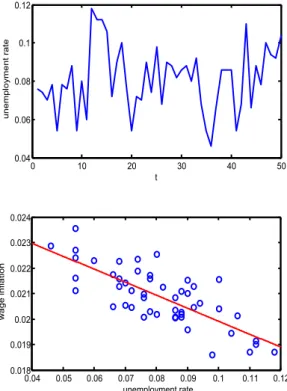
In 995 out of 1000 Monte Carlo simulations, we observe the emergence of endogenous business cycles with the statistical characteristics reported in column with η = 0 of Table 4 (see page 26). Along the typical business cycle, an increase of firms’ profits determines an expansion of production and, if banks extend the required credit, this effect could be amplified resulting in more employment; the fall of the unemployment rate increases wage inflation that, on the one hand, expands the aggregate demand, while on the other hand reduces firms’ profits, possibly causing the inversion of the business cycle. In particular, Figure 1 displays the evolution of the unemployment rate along the business cycle (upper panel) and the inverse relationship between unemployment and wage inflation, that is the Phillips curve (lower panel). In other words, there is a dynamic relation between the unemployment and the profit rate: the increase of profits boosts the expansion of the economy and then a fall of the unemployment rate follows (negative correlation between the profit rate at time t − 1 and the unemployment rate at time t). The reduced unemployment increases wages, so firms want to save on production costs (e.g., wage bill) decreasing labor demand. This results in a rise of unemployment that, in turn, reduces the profit rate at time t + 1 due to a lack of aggregate demand. However, the presence of unemployed people reduces wages and this stimulates firms to hire a larger number of workers, so boosting the beginning of a new expansionary phase of the business cycle. All in all, business cycles are basically determined by the interplay between firm leverage and the dynamics of the
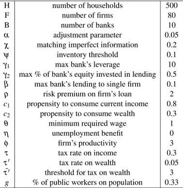
wage-Table 1: Parameter setting
H number of households 500
F number of firms 80
B number of banks 10
α adjustment parameter 0.05 χ matching imperfect information 0.2
ψ inventory threshold 0.1
γ1 max bank’s leverage 10
γ2 max % of bank’s equity invested in lending 0.5
β max bank’s lending to single firm 0.1 ρ risk premium on firm’s loan 2 c1 propensity to consume current income 0.8
c2 propensity to consume wealth 0.3
θ minimum required wage 1
η unemployment benefit 0
φ firm’s productivity 3
τ tax rate on income 0.3
τ0 tax rate on wealth 0.05 ¯
τ0 threshold for tax on wealth 3 g % of public workers on population 0.33
profit struggle (see e.g., Goodwin, 1967, Akerlof and Stiglitz, 1969): an increase in profits expands investment which in turn raises employment and wages; thus the rise in wages erodes profits and sets the premises for the recessionary phase.
In the remaining 5 out of 1000 simulations the system is characterized by large and extended crises, that is the average unemployment rate reaches values above the 20%. Differently from the usual business cycle mechanism, the decrease of wages due to growing unemployment does not reverse the cycle, but rather amplifies the recession due to the lack of aggregate demand. Indeed, real wage lowers excessively resulting in a vicious circle for which the fall of purchasing power prevents firms to sell commodities, then firms decrease production, unemployment
Figure 1: Baseline model. Simulation results 0 10 20 30 40 50 0.04 0.06 0.08 0.1 0.12 t unemp loyment rate 0.04 0.05 0.06 0.07 0.08 0.09 0.1 0.11 0.12 0.018 0.019 0.02 0.021 0.022 0.023 0.024 unemployment rate wage i nflation
continues to rise, and the recession deteriorates. In these cases, the system may remain trapped in a large crisis unless an exogenous intervention.
As for the financial aspects of the cycle, firms’ leverage and, in particular, banks’ exposure enlarge business fluctuations: when firms are growing they ask for more credit and, if banks extended new loans, then they are able to expand the production; after a while, the rise of employment fosters wages that, together with the rise of interest payments on an increasing debt, reduces firms’ profitability. Thus, the business cycle reverses and financial factors amplify the recession, indeed the relatively low level of profits with respect to interest payments induces a
deleveraging process. According to the empirical evidence (for example, Kalemli-Ozcan et al., 2011), there is a modest firms’ leverage procyclicality, while there is a more significant banks’ leverage procyclicality. Then, banks’ capitalization is the most important determinant of credit conditions, so influencing firms’ leverage and the macroeconomic evolution.
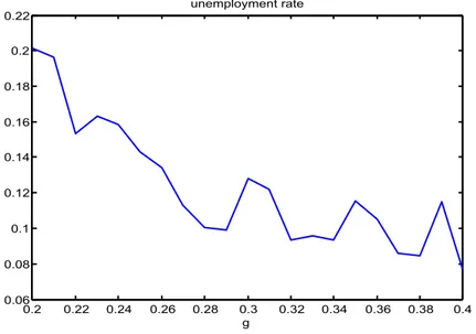
The presence of the government plays a central role in mitigating output volatility through stabilizing the aggregate demand. We show the importance of this acyclical sector with a sensitivity analysis on the parameter g (the percentage of public workers on active population): we repeat the same simulation 21 times (on time span T=150) with values of g ranging from 20% to 40%, with step 1%.4 The mean unemployment rate in the last 50 periods of the simulation (101 ≤ t ≤ 150) is reported in Figure 2. It clearly emerges that a larger acyclical sector implies a lower average unemployment rate: when g = 20% (and τ = 17%) the mean unemployment rate is above 20% (20.14%), while when g = 40% (and τ = 37%) it is below 8% (7.71%). Instead, the standard deviation of the unemployment rate does not largely change among simulations, always remaining about 2 − 3%.
The previous macroeconomic features are influenced by the peculiar aspects of the matching mechanism in various markets. We can show, with two sensitivity analyses, that the matching characteristics have different effects depending on the markets involved.
The first sensitivity analysis regards the deposit market. We compare three simula-tions with the same random seed, but with different values for the parameters α used in equations 11 and 12:
1. α = 0.05 for both equations, as in the baseline model;
2. α = 0.10 in equation 11 and α = 0.05 in equation 12; that is, the offered interest rates by banks move more rapidly than the required interest rates by household;
3. α = 0.05 in equation 11 and α = 0.10 in equation 12; that is, the required interest rates move more rapidly than the offered interest rates.
4 In order to stabilize the public deficit at a common level among the simulations (about 3%), we change at the same time also the tax rate on income τ, starting from τ = 17% to τ = 37%, with step 1% (in this way a value of g = 33% corresponds to a τ = 30%, as in the baseline setting).
Figure 2: Average unemployment rate: sensitivity analysis on parameters g (and τ) ranging from g= 20% to g = 40% (and from τ = 17% to τ = 37%), with step 1%.
0.2 0.22 0.24 0.26 0.28 0.3 0.32 0.34 0.36 0.38 0.4 0.06 0.08 0.1 0.12 0.14 0.16 0.18 0.2 0.22 unemployment rate g
Table 2 shows the mean unemployment rate and the standard deviation of the unemployment rate in the three simulations during periods 101 ≤ t ≤ 150.
Cases 1 and 2 are almost identical, then if banks and households adjust their offered and required interest rate at the same speed or if banks adjust their offered rate more rapidly has not an impact (at least till a certain threshold). Instead, if households move their required interest rate more rapidly than the rate offered by banks (simulation 3) the mismatch makes the unemployment rate to raise to 12%. The difference between cases 2 and 3 could be due to the fact that banks have an
Table 2: Sensitivity analysis about different behavioural sluggishness in the deposit market matching.
Case 1 2 3
Unemployment rate 8.42% 8.37% 12.09% Unemployment volatility 1.87% 1.77% 2.04%
upper bound in their interest rate setting given by the central bank interest rate. This may increase the fraction of liquid money hold by households, so resulting in a shrinking of banks credit supply. However, this effect that could be present in the economic reality, here is too strong due to the lack of alternative financial channels for banks to collect money (for instance bonds). All in all, the macroeconomic system behaves always in the same way, even if the mismatch could create some problems as an increase of unemployment.
The second sensitivity analysis shows how a different sluggishness in the adjustment of prices and wages (on their two different markets) can largely impact the macroeconomic system. We compare three simulations with different values for the parameters α used in equations 6 and 10:
• α = 0.05 for both equations, as in the baseline model;
• α = 0.10 in equation 6 and α = 0.05 in equation 10; that is, the required wages move more rapidly than prices;
• α = 0.05 in equation 6 and α = 0.10 in equation 10; that is, prices move more rapidly than wages, in a more realistic setting.
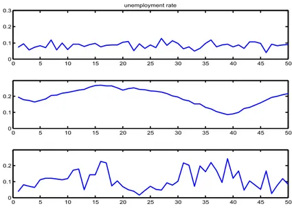
The macroeconomic system acts similarly in the baseline case and in the more realistic one, that is when prices move more rapidly than wages, but it behaves very differently in the second case (see Figure 3). Indeed, when wages move faster than prices, the system creates very long business cycles with a very high mean unemployment rate (19.42% as reported in Table 3).
The system shows a much less persistent business cycle features in the other two cases. However, when prices move faster than wages, the mean unemployment rate is larger and the business cycle volatility increases compared to the baseline case. Indeed, in the baseline case the mean unemployment rate over the 50 periods is 8.42% with a minimum of 4% and a maximum of 12.8%, while in third scenario the mean is 11.09% with a minimum of 1.6% and a maximum of 24.4%, that is with a much larger variation.
More in general, the mismatch between the two mechanism enlarges the unem-ployment (and then the output) volatility, as shown by the values reported in Table 3.
Figure 3: Unemployment rate in the three cases with different behavioural sluggishness in required wages and prices.
0 5 10 15 20 25 30 35 40 45 50 0 0.1 0.2 0.3 unemployment rate 0 5 10 15 20 25 30 35 40 45 50 0 0.1 0.2 0 5 10 15 20 25 30 35 40 45 50 0 0.1 0.2
Given the importance of this feature in the model, but also in the real economy, a more accurate analysis is required as a future development of the paper, given that the model easily allows this kind of study, as for instance a quantitative calibration of the adjustment parameters for prices and wages. Moreover, we should accurately investigate the effects of an asymmetric behaviour in the adjustment of prices and wages, as for instance in the case of downward rigidity of nominal wages. However, in what follows we focus on the role of unemployment benefits, assuming that the baseline setting can be quite representative of other cases, such as the one with
Table 3: Sensitivity analysis about different behavioural sluggishness in required wages and prices.
Case 1 2 3
Unemployment rate 8.42% 11.09% 19.42% Unemployment volatility 1.87% 5.98% 5.32%
a different sluggishness between the two sides of the deposit market or the more realistic case in which prices move more rapidly than wages.
4 Unemployment Benefits
In this Section we investigate the effects of introducing unemployment benefits (UB) in the model. As explained above, in this case the government pays a benefit to unemployed workers which is given by equation 7. In particular, we set η = 0 in the baseline model, while η = 0.5 in the UB scenario.
4.1 Baseline Model vs. Unemployment Benefit Scenario
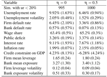
As clearly emerges from Table 4, the average rate of unemployment on 1000 Monte Carlo simulations is markedly lower in the UB scenario (about 6.5%) than in the baseline model (almost 10%), and this difference is even larger if we consider also the 5 simulations with big crises (mean unemployment rate above 20%) that we exclude from the statistics of the baseline model; indeed the big crisis scenario disappears when unemployment benefits are present (all 1000 simulations are used for the statistics in the column devoted to the UB scenario). Moreover, we observe a fall of the default rate for both firms and banks, an improvement of credit conditions (from an excess demand to an excess supply of credit in the average), an increase of both firm leverage and bank exposure, while the corresponding volatilities decrease. The negative effects of the government intervention, that is the slight increase of both the average inflation rate (from 1.99% to 2.15%) and the average ratio between the public deficit and the nominal GDP (from 3.26% to 3.37%), have a modest impact on the macroeconomy. In particular, the larger public expenditure due to providing benefits to unemployed people is quite well compensated by the increased level of taxes (with an unchanged taxation rate) deriving from a higher level of GDP in an economy with a lower rate of unemployment. Then, the government successfully intervenes in the economy through providing unemployment benefits: in this case unemployed workers can buy more goods (otherwise they can spend only a fraction of their wealth), indeed the wage share is slightly larger in the UB scenario, so increasing the demand for
Table 4: Monte Carlo for η = 0 and η = 0.5 (time span 101-150) of simulations with average unem-ployment rate below 20%. In brackets the standard deviation among the Monte Carlo simulations. We always reject the hypothesis that the two Monte Carlo means are not statistically different, with a p-value below 5%.
Variable η = 0 η = 0.5
Sim. with ur < 20% 995 1000 Unemployment rate 9.92% (1.63%) 6.46% (0.94%) Unemployment volatility 2.05% (0.48%) 1.52% (0.29%) Firm default rate 6.45% (2.10%) 3.36% (0.86%) Bank default rate 0.57% (0.57%) 0.07% (0.13%) Wage share 63.4% (0.5%) 65.2% (0.3%) Public deficit 3.26% (0.19%) 3.37% (0.14%) Interest rate 9.11% (1.93%) 7.67% (1.18%) Inflation rate 1.99% (0.07%) 2.15% (0.05%) Credit constraint on GDP 4.23% (8.13%) -6.28% (4.24%) Firm mean leverage 1.65 (0.24) 1.80 (0.24) Bank mean exposure 3.27 (1.30) 3.40 (1.12) Firm leverage volatility 0.12 (0.04) 0.09 (0.04) Bank exposure volatility 0.51 (0.33) 0.30 (0.17)
produced goods and then firms’ profits; this leads to more employment which further enlarges the aggregate demand. Furthermore, the results of the model about the role of unemployment subsidies are very complementary to previous ones in the agent-based models. In particular, the finding about the stabilizing role of unemployment subsidies into a regime where investment is profit-driven complements similar ones obtained in the models by Dosi et al. (2010, 2012), where investment is driven by expectations about demand.5
All in all, government intervention through unemployment benefits stabilizes the aggregate demand and the system is more stable despite of a higher level of both firm leverage and bank exposure. This also means that public intervention looses the credit constraint to the economy; indeed, the larger credit availability 5 For a comparison between profit-led and demand-led regimes, and an analysis of the effects of wage flexibility in the two regimes, see Napoletano et al. (2012).
results in a lower average rate of interest. In other words, a more leveraged financial sector sustains the expansion of the economy when the government provides more liquidity to the system through the countercyclical mechanism of unemployment benefits, with the fundamental cooperation of the central bank which buys the outstanding public debt.
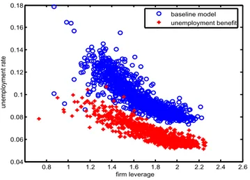
According to what explained above regarding the role of financial factors, the introduction of unemployment benefits leads to an increase of both the mean firm leverage and the mean bank exposure; moreover, for every level of both firm leverage and bank exposure we clearly observe a lower rate of unemployment, as shown in Figures 4 and 5. Another relevant aspect is the non-linear relationship that emerges in the figures. For relatively high levels of firm leverage the unemployment rate tends to be smaller and less volatile; however, for largest values of the firm leverage (above 2) the negative relation with the unemployment rate tends to disappear (Figure 4). As for banks, starting from low levels, an increase of bank exposure reduces the rate of unemployment; instead, for high levels of bank exposure (above 5) a further increase makes the unemployment higher. In other words, if banks increase their exposure enlarging credit to firms, the latter hire more workers and the unemployment rate decreases. But, when the exposure of banks becomes “excessive” this leads to instability (more defaults) and the rate of unemployment may increase (Figure 5). Moreover, in the UB scenario the relationship between the financial factors and the unemployment rate is flatter and less volatile. This confirms that the government intervention through UB reduces the unemployment rate and stabilizes the macroeconomy.
4.2 Robustness Check: Two Taylor Rules
As already explained, the government is assisted by the central bank. Till now, we have assumed that the central bank sets the policy rate iCBtat 1% and leaves it
unchanged. Now, we remove this assumption to perform a robustness check of our findings testing two different Taylor-type rules.6
Figure 4: Average unemployment rate and mean firm leverage: Monte Carlo simulations for the baseline model (‘circle’) and the unemployment benefit scenario (‘star’).
0.8 1 1.2 1.4 1.6 1.8 2 2.2 2.4 2.6 0.04 0.06 0.08 0.1 0.12 0.14 0.16 0.18 firm leverage unemp loyment rate baseline model unemployment benefit
Figure 5: Average unemployment rate and mean bank exposure: Monte Carlo simulations for the baseline model (‘circle’) and the unemployment benefit scenario (‘star’).
0 1 2 3 4 5 6 7 8 0.04 0.06 0.08 0.1 0.12 0.14 0.16 0.18 bank exposure unemp loyment rate baseline model unemployment benefit
We call the first Taylor rule a “Fed-type” rule, that is the central bank fixes a target both for unemployment and inflation:
iCBt= Πt−1+ 0.5(Πt−1− ˆΠ) + 0.5( ˆu− ut−1) (20)
where Πt−1is the inflation rate of the previous period, ˆΠ is the inflation rate target, that we fix at 2%, ut−1 is the unemployment rate of the previous period and ˆuis
the unemployment rate target, that we fix at 8%.
The second Taylor rule is an “ECB-type” rule, in which the central bank targets only the inflation rate:
iCBt= Πt−1+ (Πt−1− ˆΠ) = 2Πt−1− ˆΠ (21) Moreover we set a lower bound for the policy rate at ¯iCB= 0.5% in both cases.
We perform four (small) Monte Carlo experiments (10 simulations for each MC), applying one of the two monetary policy rules, with or without unemployment benefits.
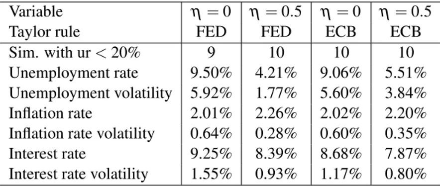
As shown by Table 5, the simulations results are quite similar to that of Table 4, even if the introduction of a Taylor-type rule in the model increases the business cycle volatility (especially if we extend the simulation, here not reported), given that in the model the duration of business cycles is quite short and central bank intervention is based on adaptive expectations, then it is very difficult for the central bank to stabilize the economy. However, we can confirm the importance of unemployment benefits also in this setting: with both rules the unemployment benefits abundantly reduces the average unemployment. This reduction appears to be larger (and with a lower unemployment volatility) when the central bank also cares about unemployment, as in the “Fed-type” rule scenario.
However, given the listed shortcomings of the above Taylor-type rule (such as the adaptive expectations of the central bank) and given the various possibilities to modify equations 20 and 21 in the weight parameters or in the inflation and unemployment target levels, we think that this topic deserves further analyses. 4.3 Sensitivity Analysis
In this Section we perform a sensitivity analysis on the parameter η that determines the size of unemployment benefits. In particular, we run 1000 simulations for 25
Table 5: 10 Monte Carlo simulations for η = 0 and η = 0.5 (time span 101-150), when the central bank applies a FED-like or a ECB-like Taylor-type rule. Statistics for simulations with average unemployment rate below 20%.
Variable η = 0 η = 0.5 η = 0 η = 0.5
Taylor rule FED FED ECB ECB
Sim. with ur < 20% 9 10 10 10 Unemployment rate 9.50% 4.21% 9.06% 5.51% Unemployment volatility 5.92% 1.77% 5.60% 3.84% Inflation rate 2.01% 2.26% 2.02% 2.20% Inflation rate volatility 0.64% 0.28% 0.60% 0.35% Interest rate 9.25% 8.39% 8.68% 7.87% Interest rate volatility 1.55% 0.93% 1.17% 0.80%
different values of η, from 0 to 2.4 with 0.1 step, then 40 replications for each step. We set θ = η so that the wage required by households is higher or at least equal to the unemployment benefit.
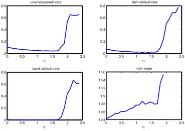
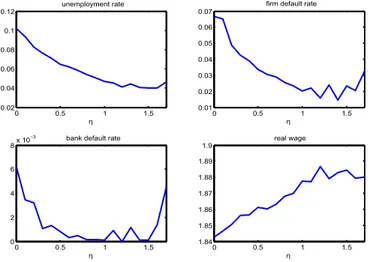
Figure 6 displays the impact of the parameter η on the following variables: (i) the unemployment rate, (ii) the firm default rate, (iii) the bank default rate, and (iv) the real wage. As it clearly emerges, for low levels of η the real wage is low and the resulting lack of aggregate demand leads to a higher number of both firms and bank defaults, and a consequent high rate of unemployment. As η increases there is a rise of the real wage and a consequent increase and stabilization of the aggregate demand, with a parallel improvement of financial conditions. This evidently confirms the results explained in the previous Section.
To better appreciate the positive impact of unemployment benefits on macroe-conomic conditions, we present the same sensitivity analysis for a reduced interval of the parameter η, that is from 0 to 1.7, in Figure 7. Looking at that figure, we can clearly see that when η is zero the unemployment rate is about 10%, the firm default rate is almost 7%, the bank default rate is around 0.6%, and the real wage is slightly higher than 1.84. As η grows until about 1.5 the system displays a decreasing rate of unemployment, a rise of the real wage, and a reduction of both the firm and the bank default rate (in the latter case there is a relevant decrease
Figure 6: Sensitivity analysis on the impact of the parameter η – from 0 to 2.4 with step 0.1 – on the unemployment rate, firm default rate, bank default rate, and real wage.
0 0.5 1 1.5 2 2.5 0 0.2 0.4 0.6 0.8 unemployment rate η 0 0.5 1 1.5 2 2.5 0 0.2 0.4 0.6
0.8 firm default rate
η 0 0.5 1 1.5 2 2.5 0 0.2 0.4 0.6
0.8 bank default rate
η 0 0.5 1 1.5 2 2.5 1.84 1.86 1.88 1.9 1.92 1.94 1.96 real wage η
until when η reaches about 0.5; after that, the number of bank defaults remains near zero till η reaches 1.5).
However, for large values of η the real wage strongly increase and the resulting profit squeeze leads to bankruptcy chains (e.g., the default rate for both firms and banks goes above 50% when η is about or more than 2) and to large crises with more than half people in the unemployment status; the consequent fall of aggregate demand reiforces the recession in a vicious circle.
Hence, the growth of η produces beneficial effects on the economy till a thresh-old of about 1.5. For higher values, the impact of η tends to reverse. Moreover, the behavior of the system radically changes when the value of η tends to approach 2. We can explain this feature of our model in the following way. When η is between 0 and about 1.8, the macroeconomy is characterized by a statistical equilibrium (as a composition of heterogeneous out-of-equilibrium behaviors of single agents) with typical business fluctuations (that is, without large crises), a reasonable rate of unemployment, quite stable financial conditions, and a real wage in the range 1.8-1.9. When the value of η is above 1.8, the intervention of the government through unemployment benefits forces the real wage to be larger than a value
Figure 7: Sensitivity analysis on the impact of the parameter η – from 0 to 1.7 with step 0.1 – on the unemployment rate, firm defualt rate, bank default rate, and real wage.
0 0.5 1 1.5 0.02 0.04 0.06 0.08 0.1 0.12 unemployment rate η 0 0.5 1 1.5 0.01 0.02 0.03 0.04 0.05 0.06 0.07
firm default rate
η 0 0.5 1 1.5 0 2 4 6 8x 10
−3 bank default rate
η 0 0.5 1 1.5 1.84 1.85 1.86 1.87 1.88 1.89 1.9 real wage η
compatible with the previously described statistical equilibrium and, therefore, the economy tends to crash.
To sum up, we observe a negative impact of the unemployment benefit on the economy only if its value is “excessive”, that is when the unemployment benefit approaches the mean real wage of employed people. Instead, for a large range below this threshold, increasing unemployment benefits clearly improves the performance of the economic system via the positive effect on the aggregate demand.
5 Concluding Remarks
We propose an agent based decentralized matching macroeconomic model that allow us to investigate the role of government intervention, based on providing unemployment benefits, in mitigating business cycle fluctuations through both improving the financial conditions of the system and sustaining the aggregate
demand. This result depends on a fruitful cooperation between the fiscal policy implemented by the government and monetary policy managed by the central bank. Our artificial macroeconomy is composed of heterogeneous agents, that is households, firms, banks, which interact in four markets (credit, labor, goods, and deposit markets), and two policy makers: a central bank and the government. Agents are boundedly rational and operate in an incomplete and asymmetric information setting by following quite simple rules of behaviour. Households buy consumption goods from the cheapest supplier, update the asked wage according to their occupational status (upward if employed, downward if unemployed), and deposit money in the bank offering a satisfactory interest rates; given Basilea-like regulatory constraints, banks extend credit to finance firms’ production; firms choose the banks offering lowest interest rates, and they are aimed at accumulating profits by selling their products to households and hiring cheapest workers. The government hires public workers, taxes private agents and issues public debt. Finally, the central bank provides money to banks, by managing the supply of money, and the government, by buying oustanding public securities.
In our macroeconomic setting, the consequence of government issuing public securities to finance unemployment benefits is twofold: (i) the public sector tranfers a benefit to unemployd people so providing an additional income to be spent, that is the aggregate demand increases due to public resources; (ii) the public sector provides liquidity to the private sector so mitigating the credit constraints to firms and then improving financial conditions. In other words, a more leveraged financial sector sustains the expansion of the economy when the government provides more liquidity to the system through the countercyclical mechanism of unemployment benefits, with the collaboration of the central bank which buys the outstanding public debt.
We think that our model can provide some suggestions to interpret, at least some aspects of, the recent evolution of economic and financial conditions in many countries, after the 2007 financial crisis and the recessive phase that followed the collapse of Lehman Brothers on September 15th, 2008. The current crisis is characterized by financial turmoil on international markets and a slowdown of economic growth in many (advanced) countries, especially in the periphery of the Euro area. The austerity strategy is boosting a recessive spiral and the aim of reaching balanced public finances seems to be impossible to obtain, at least in a
reasonable time. Indeed, cutting public expenditure and rising taxation is leading to higher unemployment in context of low confidence that results in a lack of private investment, also because the financial sector, that is banks, is not providing all the credit needed by firms to finance production, and governments are cutting public investments and the welfare state. According to the IMF, in advanced economies, stronger planned fiscal consolidation is associated with lower growth than expected early in the crisis, and this seems to be due to the fact that fiscal multipliers are substantially higher than implicitly assumed by forecasters (Blanchard and Leigh, 2013).
Moreover, financial conditions in the Euro area, as proxied by the behaviour of spreads between the interest rate paid on the 10-year German Bund and that paid on other bonds, have been improved only after the announcement of OMT (Outright Monetary Transactions) by the ECB President Mario Draghi with which the central bank can intervene on secondary markets through buying government securities if a country ask for an ESM (European Stability Mechanisms) help and then commits its fiscal policy to be subject to certain conditions to assure fiscal consolidations. This may suggest that a full operativity of the ECB, that is as a lender of last resort that can also buy outstanding public debt, can be of great help in assuring “orderly market conditions”, while instead only a commitment to the objective of a stable and moderate inflation rate may not be enough for financial stability.
Although the interplay between real and financial aspects, in the Euro area as well as in other countries, gives rise to very complex questions, which are hard to solve on the basis of the simulation results of a single model, we show that in our agent based macroeconomic setting the central bank can positively contribute to the financial stability of the system by cooperating with the government, so reinforcing the objectives of fiscal policy. Maybe, then, a high degree of cooperation between the policy makers may be thought as a possible direction to follow (that is an aspect to be reconsidered). Moreover, instead of cutting public expenditure, the government may improve the macroeconomic performance by a countercyclical action like the one based on providing unemployment benefits, taking care of avoiding an excessive intervention that may instead squeeze profits and lead the economy towards recession.
As for future research, our aim is twofold. On one hand, we want to enrich the present analysis. For instance, instead of using unemployment benefits, the government could carry out a countercyclical policy enlarging and reducing the fraction of public workers, considering the public sector as an “employer of last resort” along the Minskian tradition (Wray, 2007). We can suppose that both interventions make the aggregate demand to rise, but they probably present also different features. The strategy to hire a countercyclical fraction of public workers could enlarge the economic production (and reduce the labor productivity loss of unemployed households), but it could be less effective in restoring private sector’s production, given that there would be less unemployed workers available to private firms with a reasonable required wage (above the unemployment benefit, but below the wage paid by the government). However, to analyse the different scenarios with both kind of interventions, evaluating the gains for firms due to increased aggregate demand versus increased costs, but also the productivity gains for the whole society, we need a richer model.
On the other hand, indeed, we want to further extend our macroeconomic setting. Then, we will introduce new markets, for instance a market for invest-ment goods, a mechanism of technological progress underlying economic growth, heterogeneous rules of consumption and the possibility of consumer credit, more complicated financial behavior based on managing portfolio choices, a varying number of actors (firms and banks) during the business cycle, different decisional timings (and frequency) in the various markets, and so on, in order to develop a useful tool for interpreting the evolution of economic and financial conditions and to analyze policy issues. With a more complete model, it will also be possible to better quantitatively calibrate a number of macroeconomic features.
References
[1] Acemoglu, D., and Shimer, R. (2000) Productivity Gains from Un-employment Insurance, European Economic Review 44(7): 1195–1224.
http://ideas.repec.org/a/eee/eecrev/v44y2000i7p1195-1224.html
[2] Adrian, T., and Shin, H.S. (2008) Liquidity, Monetary Policy and Financial Cycles, Current Issues in Economics and Finance 14(1), Federal Reserve Bank of New York (January/February).
[3] Adrian, T., and Shin, H.S. (2009), Money, Liquidity, and Monetary Policy, American Economic Review99(2): 600–605.
http://ideas.repec.org/a/aea/aecrev/v99y2009i2p600-605.html
[4] Adrian, T., and Shin, H.S. (2010), Liquidity and Leverage, Journal of Finan-cial Intermediation19(3): 418–437.
http://ideas.repec.org/a/eee/jfinin/v19y2010i3p418-437.html
[5] Akerlof, G.A., and Stiglitz J.E. (1969), Capital, Wages and Structural Unem-ployment, Economic Journal 79(314): 269–281.
http://ideas.repec.org/a/ecj/econjl/v79y1969i314p269-81.html
[6] Allsopp, C., and Vines, D. (2000), The Assessment: Macroeconomic Policy, Oxford Review of Economic Policy16(4): 1–32.
http://ideas.repec.org/a/oup/oxford/v16y2000i4p1-32.html
[7] Ashraf, Q., Gershman B., and Howitt, P. (2013), How Inflation Affects Macroeconomic Performance: An Agent-Based Computational Investigation, Macroeconomic Dynamics, forthcoming.
[8] Bender, S., Schmieder, J., and Von Wachter, T. (2009), The Long-Term Impact of Job Displacement in Germany During the 1982 Recession on Earnings, Income, and Employment, Department of Economics Discussion Paper Series DP0910-07, Columbia University.
[9] Blanchard, O., and Leigh, D. (2013), Growth Forecasts Errors and Fiscal Multipliers, IMF Working Paper, WP/13/1, Research Department, Interna-tional Monetary Fund.
http://www.imf.org/external/pubs/cat/longres.aspx?sk=40200.0
[10] Booth, L., Asli Demirgu-Kunt, V.A., and Maksimovic, V. (2001), Capi-tal Structures in Developing Countries, Journal of Finance 56(1): 87–130.
http://onlinelibrary.wiley.com/doi/10.1111/0022-1082.00320/abstract
[11] Brunnermeier, M.K., and Pedersen, L.H. (2009), Market Liquidity and Funding Liquidity, Review of Financial Studies 22(6): 2201–2238.
http://ideas.repec.org/a/oup/rfinst/v22y2009i6p2201-2238.html
[12] Challe, E., Charpe, M., Ernst, E., and Ragot, X. (2011), Countercyclical Un-employment Benefits and UnUn-employment Fluctuations, International Labour Organization.
[13] Cincotti, S., Raberto, M., and Teglio, A. (2010), Credit Money and Macroe-conomic Instability in the Agent-Based Model and Simulator Eurace, Eco-nomics: The Open-Access, Open-Assessment E-Journal, Vol. 4, 2010-26.
http://dx.doi.org/10.5018/economics-ejournal.ja.2010-26
[14] Cincotti, S., Raberto, M., and Teglio, A. (2012), Debt Deleverag-ing and Business Cycles. An Agent-Based Perspective, Economics: The Open-Access, Open-Assessment E-Journal, Vol. 6, 2012-27.
http://dx.doi.org/10.5018/economics-ejournal.ja.2012-27
[15] Dawid, H., and Neugart, M. (2011), Agent-Based Models for Economic Policy Design, Eastern Economic Journal 37(1): 44–50. http://www.palgrave-journals.com/eej/journal/v37/n1/abs/eej201043a.html
[16] Deissenberg, C., van der Hoog, S., and Dawid, H. (2008), EU-RACE: A Massively Parallel Agent-based Model of the European Economy, Applied Mathematics and Computation 204: 541–552.