Col.lecció d’Economia E19/394
Agricultural Composition and Labor
Productivity
Cesar Blanco
Xavier Raurich
UB Economics Working Papers 2019/394
Agricultural Composition and Labor Productivity
Abstract: Labor productivity differences between developing and developed countries
are much larger in agriculture than in non-agriculture. We show that cross-country differences in agricultural composition explain a substantial part of labor productivity differences. To this end, we group agricultural products into two sectors that are differentiated only by capital intensity. As the economy develops and capital accumulates, the price of labor-intensive agricultural goods relative to capital-intensive agricultural goods increases. This price change drives a process of structural change that shifts land and farmers to the capital-intensive sector, increasing labor productivity in agriculture. We illustrate this mechanism using a multisector growth model that generates transitional dynamics consistent with patterns of structural change observed in Brazil and other developing countries, and with cross-country differences in agricultural composition and labor productivity. Finally, we show that taxes and regulations that create a misallocation of inputs within agriculture also reduce the relative labor productivity.
JEL Codes: O41, 047.
Keywords: Structural change, Agriculture labor productivity, Capital intensity.
Cesar Blanco
Central Bank of Paraguay Xavier Raurich
Universitat de Barcelona
Acknowledgements: Financial support from the Government of Spain through grant RTI2018-093543-B-I00 and from the Central Bank of Paraguay is gratefully acknowledged. This paper has benefited from comments by participants in the 43rd Symposium of the Spanish Economic Association, the 2018 Society for Economic Dynamics meeting (Mexico), the Public Economic Theory meeting (Vietnam), the XI Workshop on Public Policy Desing (Girona) and the seminars at the Universities of Vienna and Guanajuato.
.
1
Introduction
A recent strand of the growth literature claims that a substantial part of cross-country in-come di¤erences can be explained by di¤erences in agricultural labor productivity between
developing and developed countries.1 This claim is based on two observations. First,
la-bor productivity di¤erences between developed and developing countries are much larger in agriculture than in non-agriculture. Second, employment in agriculture is still large in de-veloping countries. In particular, Lagakos and Waugh (2013) report that agricultural labor productivity in countries in the 90th percentile of the world income distribution is 45 times larger than that of countries in the 10th percentile of the distribution. In contrast, non-agricultural labor productivity is only 4 times larger in advance countries. This implies that labor productivity of agriculture relative to non-agriculture increases along the development process.
A central issue is therefore to explain the increase of the labor productivity in agricul-ture relative to non-agriculagricul-ture along the development path. To account for this pattern, the literature has introduced misallocations of production factors (Chen, 2017; Gottlieb and Grobovsek, 2015; Hayashi and Prescott, 2008; Restuccia et al., 2008; Restuccia and Santaeulalia-Llopis, 2017), di¤erences in farm sizes (Adamopoulos and Restuccia, 2014), dif-ferences in technology (Chen, 2017; Gollin et al., 2007; Manuelli and Seshadri, 2014; Yang and Zhu, 2013), selection (Lagakos and Waugh, 2013), uninsurable risk and incomplete cap-ital markets (Donovan, 2016), and di¤erences in the quality of capcap-ital (Caunedo and Keller, 2016).
In the literature cited above, it is argued that misallocations of production factors di-minish as economies develop. This can lead to an increase in both agricultural and relative labor productivity. This process is ampli…ed by structural change and selection. That is, as structural change takes place, farmers that leave the agricultural sector …rst are those endowed with lower abilities for farming. The remaining farmers are endowed with higher abilities, giving rise to higher labor productivity in this sector. In addition, as the number of farmers declines due to structural change, there is an increase in the average size of farmers that increases labor productivity in this sector. Finally, economic development and capital accumulation allow an improvement in the quality of capital and a shift from a labor in-tensive technology to a capital inin-tensive one. As a result, labor productivity in agriculture increases with better capital and a more capital intensive technology.
The aforementioned literature considers an aggregate agricultural sector producing a single commodity. It disregards the fact that agricultural products are diverse, that they can be produced with di¤erent technologies, and that the consumption composition of these products can change along economic development. In this paper, we identify a process of substitution of crops associated with development, which we denote as structural change within agriculture, and study how this process contributes to explain the observed increase in the relative labor productivity.
We use the US Census of Agriculture and the Food and Agriculture Organization (FAO) datasets to group crops into two di¤erent sectors: a capital intensive and a labor
inten-1See Chanda and Dalgaard (2008), Cao and Birchenall (2013), Caselli (2005), Gollin et al. (2002), Gollin
sive agricultural sector. The mechanism relating changes in agricultural composition and relative productivity is as follows. As the economy develops and capital accumulates, the relative price of labor intensive crops to capital intensive crops increases. If the two crops are imperfect substitutes in preferences, the production of labor intensive crops relative to capital intensive crops declines. As a consequence, aggregate agriculture becomes more
cap-ital intensive, which reduces the amount of farmers and increases the average farm size.2
Therefore, an increase of labor productivity in agriculture can be explained by: an increase in capital intensity, higher average farm size, and a reduction in the number of farmers.
We introduce this mechanism in a multisector overlapping generations (OLG) model, in which a continuum of individuals is born in each period. These individuals have hetero-geneous agricultural skills and homohetero-geneous ability for non-agricultural work. As in Lucas (1978), young individuals with low abilities choose to become workers, whereas individu-als with high abilities become entrepreneurs. In our framework, workers are employed in non-agriculture, while entrepreneurs are farmers specialized in the production of either land or capital intensive crops. Since technologies exhibit complementarity between ability and capital, only farmers endowed with high abilities choose to produce capital intensive crops. When old, individuals are retired and consume both an agricultural and a non-agricultural good subject to a minimum consumption requirement in agriculture. The agricultural good is de…ned as a constant elasticity of substitution (CES) aggregate of the goods produced in the two agricultural sectors.
Young individuals accumulate capital in order to consume when old. Capital accumu-lation and exogenous technological progress drive economic growth which generates two di¤erent processes of structural change: between sectors and within agriculture. First, to account for structural change between sectors we consider a minimum consumption require-ment. This introduces an income e¤ect which reduces the size of agriculture and the number of farmers, as a result of economic growth. The remaining farmers have higher abilities and larger farms. This is consistent with evidence provided by Adamopoulos and Restuccia (2014), who report that the average farm size in the 20% poorest countries in the world is 34 times smaller than in the 20% richest countries. It is also consistent with Lagakos and Waugh (2013), who argue that selection ampli…es labor productivity di¤erences between sectors. Second, structural change within agriculture is explained by an increase in the price of labor intensive crops relative to capital intensive crops, which is a result of capital accu-mulation and di¤erences in capital intensity. As agriculture becomes more capital intensive, labor productivity in agriculture is bene…ted. This second process of structural change and its relation with labor productivity in agriculture are the main contributions of this paper.
The model is calibrated to match data from Brazil and we use it to simulate the dynamic
transition to the steady state.3 Along the transition, the economy develops, capital
accu-mulates and the price of labor intensive crops relative capital intensive crops increases. The
2The increase in capital intensity in agriculture relative to non-agriculture, along the process of economic
development, is consistent with evidence provided by Chen (2017) and Alvarez-Cuadrado et al. (2017). In particular, Chen (2017) indicates that the capital-output ratio in agriculture is 3.2 times larger in developed countries than in developing countries, whereas it is only 2.1 times larger in non-agriculture.
3The transitional dynamics implied by the convergence to the steady state from an initially low capital
stock is equivalent to one generated by a single technological shock that a¤ects all sectors and drives a transition between two steady states that only di¤er in the level of technology.
relative price change drives a process of structural change that implies: (i) a reduction in the number of farmers, mainly in the labor intensive sector; (ii) an increase in the average farm size; (iii) an increase in the fraction of harvested land used in the capital intensive sector; and (iv) an increase in the capital intensity of the agricultural sector relative to the non-agricultural sector. Higher average farm size and agricultural capital intensity lead to higher labor productivity in agriculture relative to non-agriculture. We show that this de-velopment patterns are consistent with the patterns of structural change observed in Brazil and other developing countries during the period 1960-2014. Moreover, we show that the model accounts for 41% of the observed increase in the relative labor productivity of Brazil during this period.
In addition, we provide cross-country evidence for a large sample of countries, including developing and developed countries, supporting the patterns of development implied by our model. More precisely, the cross-country data shows a positive correlation between (i) GDP per capita and the fraction of harvested land in capital intensive agriculture, and (ii) between this fraction and relative labor productivity. We calibrate our model to match data from countries at the high end of the income distribution and introduce aggregate productivity shocks to match GDP and the fraction of land in capital intensive agriculture of countries in the remaining quartiles of the income distribution. We …nd that our mechanism accounts for 29% of di¤erences in relative productivity observed between countries in the …rst and second quartile, and 27% of di¤erences observed between countries in the second and third quartile.
Finally, we study the e¤ect of ine¢ ciencies that generate a misallocation of agricultural production inputs between agricultural sectors and, therefore, reduce relative labor produc-tivity. We denote this form of ine¢ ciency as misallocation of agricultural composition. First, we consider the e¤ect on the labor productivity of di¤erent taxes. The development literature has shown that sector speci…c taxes that cause a wedge between wages in agriculture and non-agriculture a¤ect the relative labor productivity. We extend this analysis by showing that taxes that modify the sectoral composition of the agricultural sector also have a sig-ni…cant e¤ect on the relative labor productivity, even if these taxes do not produce a direct wedge between income in agriculture and non-agriculture. Finally, we consider a di¤erent type of ine¢ ciency, a regulation that prevents workers from leaving the agricultural sector. This regulation bene…ts the labor intensive agricultural sector, by avoiding structural change within agriculture, which keeps relative labor productivity low.
This paper is related to three strands of the literature. First, it relates to the struc-tural change literature that introduces income and price e¤ects to explain changes in the sectoral composition of an economy (see Kongsamut et al., 2001; Ngai and Pissarides, 2007; and Guerrieri and Acemoglu, 2008). We consider price and income e¤ects to account for structural change between broad sectors and within agriculture.
Second, it relates to the literature that studies increases in the capital intensity of agri-culture relative to non-agriagri-culture resulting from technological change (see Gollin et al., 2007 and Alvarez-Cuadrado et al., 2017). In particular, it is related to Chen (2017) who links in-creases in both capital intensity and average farm size to changes in technology. In contrast, in our paper the increase in capital intensity is not a consequence of technological change, but of substitution among crops. This is an important di¤erence that a¤ects not only the model, but the targets of calibration. In the technological change literature, the model is
calibrated to match a technological adoption curve or a measure of capital intensity. Instead, we calibrate the model to account for structural change within the agricultural sector.
Finally, it relates to the literature on misallocations that studies how ine¢ ciencies gen-erate a misallocation of di¤erent production factors between broad economic sectors (see Hayashi and Prescott, 2008 and Restuccia et al., 2008). We contributed to this literature by showing how ine¢ ciencies can create a misallocation of resources within agricultural sectors and how this a¤ects relative labor productivity.
The rest of the paper is organized as follows. Section 2 shows the empirical strategy followed to construct the two agricultural subsectors. Section 3 introduces the model, while Section 4 characterizes the equilibrium. Section 5 shows the results from the simulation of the model. Section 6 introduces misallocations of production factors. Finally, Section 7 concludes.
2
Agricultural sectors
We use the US Census of Agriculture to obtain the ratio between capital and value added by
crop, which is a standard measure of capital intensity.4 Table 1 shows the value of this ratio
for di¤erent years in which the census is available and for four main crop categories under
the North American Industry Classi…cation System (NAICS).5 Although there are some
important changes in capital intensity among censuses, a clear pattern emerges: the …rst two categories, Oilseed and grain farming and Other crop farming, have a capital intensity that, on average, is larger than 1.5, whereas the last two categories, Vegetable and melon farming and Fruit and tree nut farming, have an average ratio of about 0.5. Therefore, there is a large and persistent gap in the capital intensities across di¤erent categories of crops.
This gap remains if we consider the capital intensity of crops within categories. Table 2 shows that capital intensity, de…ned as the ratio between capital and production, of crops in the upper two categories is in general larger than capital intensity of any crop in the bottom
two categories.6 Given these …ndings, we distinguish between two types of agricultural
sectors. Crops in the …rst two categories of Table 1 belong to capital intensive agriculture, whereas crops in the other two categories belong to labor intensive agriculture. We assume that this classi…cation remains stable through time and across countries.
Next, we use the Food and Agriculture Organization (FAO) dataset, that provides crop level data on production, prices and area harvested for a large number of countries. We consider the period 1961-2014. Using the classi…cation of crops obtained from the US census, we classify 94 crops in the FAO dataset in order to construct the two agricultural sectors.
4We compute the value added as the market value of crops excluding government payments and
ex-penditures in fertilizers, chemicals, seeds, gasoline, utilities, supplies, maintenance and all other production expenses. Capital is de…ned as the value of equipment and machinery.
5We use census data for the following years: 1978, 1982, 1992, 1997, 2002, and 2012. The …rst 3 censuses
use the Standard Industrial Classi…cation system (SIC); however, we can still classify them according to cathegories following NAICS. Note also that Table 1 does not include hay, nor greenhouse and ‡oriculture production, which are crops not considered in the FAO dataset.
6At crop level, the US Census of Agriculture provides data on production and capital. Therefore, we
compare the ratio between capital and production, instead of capital and value added which is the standard measure of capital intensity.
This gives us the value of production, the price index and the fraction of total harvested land in each sector, for each country and time period. The classi…cation of crops is shown in the appendix.
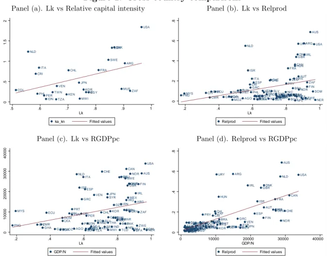
In Figure 1, we show cross-country empirical evidence on the relation between harvested land in capital intensive agriculture and other variables of interest. In particular, Panel (a) of Figure 1 shows a positive correlation between the fraction of harvested land in capital intensive agriculture and relative capital intensity between agriculture and non-agriculture.
Relative capital intensity is available for 25 countries.7 Although data is limited, we obtain a
positive correlation that is statistically signi…cant at 3%. This positive correlation provides indirect support to our classi…cation of crops: economies with a larger capital intensive agricultural sector have a more capital intensive agriculture relative to the non-agricultural sector.
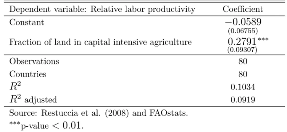
According to the mechanism described in the introduction, the share of capital intensive agriculture increases as the economy develops. As a consequence, the labor productivity of aggregate agriculture in relation to non-agriculture should also increase. Therefore, this mechanism implies a positive correlation in the data between: (i) the fraction of harvested land in capital intensive agriculture and GDP per capita; (ii) between this fraction and relative labor productivity; and (iii) between GDP per capita and relative productivity. Panels (b), (c) and (d) of Figure 1 illustrate these three positive correlations, using the cross-country comparable measure of relative productivity provided in Restuccia et al. (2008). This sample includes 80 countries for the year 1985. Tables 3, 4 and 5 show that these three positive correlations are statistically signi…cant. To complete this analysis, we run a linear regression between relative labor productivity and the fraction of harvested land in
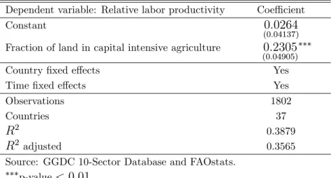
capital intensive crops, using a panel data of 37 countries during the period 1961-2011.8 The
data on relative productivities does not consider PPP prices; therefore, it is not-directly comparable across countries. This justi…es the introduction of country and time …xed e¤ects in the regression. The results are displayed in Table 6, they show a positive and statistically signi…cant correlation. We conclude that the empirical evidence available provides support to our mechanism.
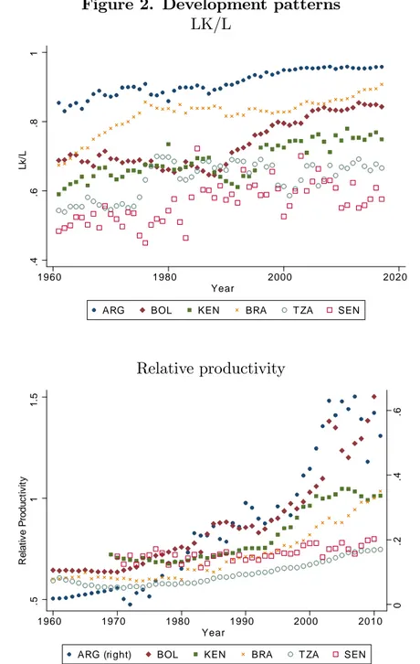
In Figure 2, we provide time series evidence for selected countries. The …gure shows developing countries that exhibited a process of development in which the fraction of har-vested land in capital intensive crops and the relative productivity increased. Among these countries, we select Brazil to calibrate the model and perform numerical simulations.
We choose Brazil because it is a large country with a diversi…ed agricultural sector that exhibited the classical patterns of development: an increase in capital intensity, structural change and a large increase in relative labor productivity. These patterns are displayed in Figure 3, for the period 1961-2014. The …gure shows that the relative price between labor and capital intensive sectors exhibits large ‡uctuations and a rising trend, whereas the relative production between these two sectors declines. This evidence suggests imperfect
7Relative capital intensity in Figure 1 is de…ned as capital per worker in agriculture divided by capital
per worker in non-agriculture. Capital by sector is obtained from Larson et al. (2000). It is combined with employment data from the GGDC 10-Sector Database.
8Data on relative labor productivity is obtained from the GGDC 10-Sector Database. We exclude 5
countries for wich data is unavailable during the entire period (Germany, Hong-Kong, Ethiopia, Mauritius and Singapore) .
substitution in consumption between agricultural goods.9 At this point, we clarify that production is not measured in value added terms, hence, it cannot be used to calibrate the model. The …gure also shows that the ratio of capital to GDP has increased and, more importantly, that Brazil has experienced two important patterns of structural change. First, structural change across sectors, which is measured by the fraction of total employment in agriculture. This fraction exhibits a major decline during this period, from 55% to 16%. Second, there is structural change within agriculture, which is measured by the fraction of total land in the labor intensive sector. It also exhibits a pronounced decline, from 30% to 10%. Finally, the relative labor productivity in Brazil has experienced a considerable increase of 27% points, from 8% to 35%. The purpose of our paper is to measure how much of this increase is explained by the patterns of structural change.
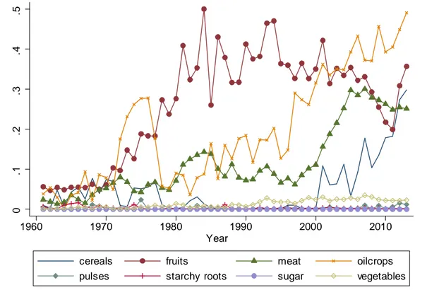
In this paper, the driver of structural change is domestic consumption demand that shifts the sectoral composition along the development process. Alternatively, another po-tential driver of structural change, not considered in our analysis, are exports of agricultural products. Therefore, we …rst show that exports are not an important driver of structural change within the agricultural sector in Brazil. To this end, Figure 4 shows the evolution of agricultural exports as percentage of production for main agricultural products in Brazil. Note that we include exports of meat, as they could indirectly drive demand for cereals and oil seeds, that is, capital intensive agricultural products. The …gure shows that products with high agricultural exports are meat, cereals, fruits and oil crops. Exports of meat and cereals rise after 2000 and, therefore, the increase is posterior to the period 1960-1980, in which the land in the capital intensive sector experiences the larger increase. Exports of fruits, that corresponds to labor intensive crops in our classi…cation, increase substantially during the period 1970 to 1984 and remain stable, or even slightly decline, after that period. The increase in exports of fruits coincides with a slight reduction in the fraction of harvested land in the capital intensive sector. Therefore, exports of fruits may explain the interruption in the process of structural change in the agricultural sector that occurs in Brazil between mid 1970 and the end of the eighties. Finally, oil crops exhibit a temporary increase dur-ing the period 1972-1977 that completely vanished after 1977. Since 1997, exports of oil crops increase steadily from 14.8% to 49.1% of production. Almost all exports of oil crops correspond to soybeans, which is an important agricultural product in Brazil.
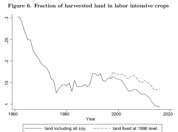
In order to illustrate the importance of soybeans, Figure 5 shows the fraction of harvested land used in the main agricultural crops from 1961 to 2017. Clearly, the most striking development is the increase in soybeans that currently accounts for 43.1% of total harvested land. We distinguish between two sub-periods in the evolution of the fraction of harvested land in soybeans. The …rst sub-period is 1961-1996, in which the fraction of harvested land moves from 0.9% to 22.1%. During this period exports are low, on average 18% of total production, and they have no clear trend. In the second period, 1997-2017, land in soybeans increases from 22.1% until 43.1%. During this period exports are large, on average 40% of production, and the trend is clearly rising. The existence of this second period, in which international trade is crucial to explain the evolution of soybeans, motivates the analysis in Figure 6. In this …gure, we compare the observed fraction of harvested land in labor
9The construction of the two agricultural sectors implies perfect substitution of crops within each
intensive crops with he fraction that would be obtained if we kept land in soybeans …xed at 1996 levels, that is, before the rise of exports started. From this comparison, we can observe that the e¤ect of soybeans’exports on the process of structural change within agriculture is not particularly important when during full period.
We conclude from this analysis that, although agricultural exports contribute to explain the rise of capital intensive agriculture in Brazil, they are not the main driver of structural change. This justi…es a study of Brazil in the following sections, in which we present a multisector growth model of a close economy and analyze how structural change can explain an increase in relative labor productivity.
3
Model
3.1
Individuals
The economy is populated by a continuum of individuals of mass one. Individuals live for two periods. When young, they choose the sector of activity, they work and they save buying capital and land. When old, they consume the accumulated savings. Young individuals are
di¤erentiated by their ability in agriculture, which we denote by ai. In every generation, these
abilities follow the same Pareto distribution with density function f (ai) = (ai) (1+ )and
cumulative function F (ai) = 1 ( =ai) . In addition, we assume that all individuals have
the same ability for non-farm work.
An individual i derives utility from consumption in the second period of his life according to the following non-homothetic utility function:
Uti = ! ln cia;t+1 c + (1 !) ln cin;t+1; (1)
where ci
a;t+1 is the consumption of agricultural goods, cin;t+1 is the consumption of
non-agricultural goods, c is a subsistence level of non-agricultural consumption, and ! 2 (0; 1) is the weight of agricultural consumption in the utility function. The agricultural good is de…ned as the following aggregate of goods produced in the capital and in the labor intensive sectors:
cia;t+1 = h ciL;t+1 " 1 " + (1 ) ci K;t+1 " 1 " i " " 1 ; (2)
where 2 (0; 1) is the weight of labor intensive goods, and " > 0 is the elasticity of
substitution between the consumption of labor intensive agricultural goods, ciL, and capital
intensive agricultural goods, ci
K.
Let total consumption expenditure be de…ned as
Et+1i Pn;t+1cin;t+1+ PL;t+1ciL;t+1+ PK;t+1ciK;t+1; (3)
where PL;t+1 is the price of the labor intensive goods, PK;t+1 is the price of the capital
intensive goods and Pn;t+1 = 1 for all t, since the output of the non-agricultural sector
obtained from maximizing utility subject to (3) (derivation in Appendix A): ciL;t+1= ! " PL;t+1 Pa;t+1 1 " Ei t+1 PL;t+1 + (1 !) " PL;t+1 Pa;t+1 " c; (4) ciK;t+1 = ! (1 )" PK;t+1 Pa;t+1 1 " Ei t+1 PK;t+1 + (1 !) (1 )" PK;t+1 Pa;t+1 " c; (5) cin;t+1= (1 !) Et+1i (1 !) Pa;t+1c; (6) where Pa;t+1 "PL;t+11 " + (1 )"PK;t+11 " 1 1 ": (7)
3.2
Technology
We distinguish between three production sectors: two agricultural and one non-agricultural. Firms in the non-agricultural sector produce combining capital and labor according to the following constant returns to scale production function:
Yn;t = AnKn;tnN
1 n
n;t ; (8)
where Yn;t is output in non-agriculture, An is a productivity parameter, Kn;t is the capital
stock employed in this sector, Nn;t is the total amount of labor employed in this sector and
n 2 (0; 1) is the capital-output elasticity. We assume that capital completely depreciates
after one period. We also assume perfect competition and, hence, the wage and the rental price of capital satisfy
wt = (1 n) AnKn;tnN
n
n;t ; (9)
and
Rt = nAnKn;tn 1Nn;t1 n: (10)
As capital completely depreciates, the rental price of capital satis…es Rt= 1 + rt, where rtis
the interest rate. Finally, it will be useful for our analysis to rewrite (9) and (10) as follows:
wt= n 1 n n (1 n) A 1 1 n n R n n 1 t (11)
Individuals working in agriculture are the owners of the farms. Farmers can produce either labor or capital intensive crops using the following technology:
yis;t = Asai Lis;t
s
Ks;ti s
; (12)
where yi
s;t is the output produced by a farmer with ability ai in the agricultural sector s,
As is the productivity parameter, Lis;t and Ks;ti are the amount of land and capital that a
farmer with ability ai rents,
s 2 (0; 1) measures the land output elasticity and s 2 (0; 1)
measures the capital output elasticity. The subindex s equals L when we consider the labor intensive agricultural sector and K when we consider the capital intensive sector.
We assume that s+ s < 1, hence, the production function exhibits decreasing returns
to scale and farmers make positive pro…ts that can be interpreted as the labor income of the farmer. Pro…t is given by
i
where xt is the rental cost of land, 2 (0; 1) is a tax on agricultural production and > 0is a tax on the rental cost of capital used in the agricultural sector. These two taxes amount for di¤erent agricultural speci…c ine¢ ciencies that reduce relative labor productivity, as we will discuss in Section 6. The farmers’optimal demands of land and capital are
Lis;t = " s (1 + ) Rt s s xt 1 s (1 ) Ps;tAsai # 1 1 s s ; (14) Ks;ti = " s (1 + ) Rt 1 s s xt s (1 ) Ps;tAsai # 1 1 s s ; (15)
and the amount produced is
ys;ti = Asai " s (1 + ) Rt s s xt s (1 ) Ps;tAsai s+ s # 1 1 s s : (16)
Note that the size of a farm, measured by Li
s;t, increases with farmer’s ability, but
de-creases with the cost of land. Finally, we replace (14), (15) and (16) in the pro…t function to obtain i s;t a i = (1 s s) " s (1 + ) Rt s s xt s (1 ) Ps;tAsai # 1 1 s s : (17)
We assume that K + K > L+ L; which implies that the fraction of after tax value of
production that the farmer obtains as income is larger in labor intensive agriculture.
3.3
Individuals’decisions
Young individuals’ decision regarding the sector where they work depends on their abili-ties. To understand this decision, we …rst obtain the ability of the two marginal individuals that are indi¤erent between two sectors of activity. The …rst marginal individual is indif-ferent between working in non-agriculture and labor intensive agriculture. We denote by
at the ability of this individual. This ability is obtained from solving the following
equa-tion: iL;t(at) = (1 ) wt; where 2 (0; 1) is a labor income tax that workers in the
non-agricultural sector must pay. We …nd that
at= 1 (1 ) PL;tAL (1 ) wt (1 L L) 1 L L xt L L (1 + ) R t L L : (18)
We denote by atthe ability of the second marginal individual, who is indi¤erent between
the following equation: i L;t(at) = iK;t(at). We obtain at= 1 K K 1 L L (1 L L)(1 K K) L+ L K K K (1+ )Rt K K xt K (1 ) PK;tAK 1 L L L+ L K K L (1+ )Rt L L xt L (1 ) PL;tAL 1 K K L+ L K K (19)
The assumption L+ L< K+ K implies that the pro…t function of capital intensive
farms as a function of abilities is stepper at ai = at than that of labor intensive farms.
Given that individuals maximize their labor income, it follows that we can only have both
types of farms if at > at: Therefore, as shown in Figure 7, individuals with ai 2 [ ; at] will
be workers in the non-agricultural sector, individuals with ai 2 [at; at] will be farmers in
the labor intensive sector and individuals with ai
2 [at;1] will be farmers in the capital
intensive sector. Note that if at< atthen all farmers will produce capital intensive crops. In
our simulations, the condition at> atwill always be satis…ed along the dynamic equilibrium.
Finally, the assumption L+ L < K + K also implies that the marginal individual
satis…es PLyL;ti (at) < PKyK;ti (at). Thus, there is a productivity gain when the marginal
farmer moves from the labor to the capital intensive sector.
4
Equilibrium
In this section, we characterize the equilibrium of the model. To this end, we obtain aggregate consumption demand, aggregate input demands and aggregate supply of output. Regard-ing consumption demands, note that old individuals consume income they generated when young. It follows that young individuals save all their income by buying capital and land. Therefore, the consumption expenditure of an old individual that was a non-agricultural
worker in period t is Et+1n;i = Rt+1[(1 ) wt+ Ti] ; where Ti is a transfer from the
govern-ment. The consumption expenditure of an old individual that was a labor intensive farmer
is Et+1L;i = Rt+1 iL;t(ai) + Ti . Similarly, the consumption expenditure of an old individual
that was a capital intensive farmer is Et+1K;i = Rt+1 iK;t(ai) + Ti . It follows that aggregate
consumption expenditure is given by
Et+1= Z at Et+1n;if ai di + Z at at Et+1L;if ai di + Z 1 at Et+1K;if ai di: (20)
We assume that tax revenues are returned to individuals as a transfer and the government budget constraint is balanced in each period, hence,
1 Z Tif ai di = Z at wtf ai di+ Z at at PL;tyL;ti + RtKL;ti f a i di + Z 1 at PK;tyK;ti + RtKK;ti f a i di:
Using the government budget constraint and (20), we obtain Et+1 = Rt+1 8 > > > > > > < > > > > > > : n 1 n n (1 n) A 1 1 n n R n n 1 t h 1 ( =at) i + 1 1 L 1+L L (1+ )Rt L L xt L (1 ) PL;tAL 1 1 L L L;t + 1 1 K 1+K K (1+ )Rt K K xt K [(1 ) PK;tAK] 1 1 K K K;t 9 > > > > > > = > > > > > > ; ; (21)
where L;t and K;t are both positive only when > 1= (1 K K) (derivation in
Appendix B). We assume this condition in the numerical exercises below.
Given that the utility function in the model belongs to the class of Gorman preferences, the aggregate demand of the di¤erent consumption goods does not depend on the distribution of consumption expenditures, but on aggregate consumption expenditure only. Using (4), (5) and (6), we obtain aggregate consumption of labor and capital intensive agricultural goods and of non-agricultural goods that, respectively, are given by
CL;t+1 = ! " PL;t+1 Pa;t+1 1 " Et+1 PL;t+1 + (1 !) " Pa;t+1 PL;t+1 " c; (22) CK;t+1 = ! (1 ) " PK;t+1 Pa;t+1 1 " Et+1 PK;t+1 + (1 !) (1 )" Pa;t+1 PK;t+1 " c; (23) Cn;t+1 = (1 !) Et+1 (1 !) Pa;t+1c: (24)
Using (14) and (15), we obtain the following aggregate demands of land and capital in
each agricultural sector:10
Ls;t = " s (1 + ) Rt s s xt 1 s (1 ) Ps;tAs # 1 1 s s s;t; (25) and Ks;t = " s (1 + ) Rt 1 s s xt s (1 ) Ps;tAs # 1 1 s s s;t; (26)
We use (10) to obtain the demand of capital in the non-agricultural sector:
Kn;t= nAn Rt 1 1 n Nn;t; (27)
where the amount of workers in this sector is given by Nn = F (a) = 1 a . The total
stock of capital, K, satis…es
Kt= KL;t+ KK;t+ Kn;t: (28)
10Equation (25) is obtained following a procedure similar to the one in Appendix B and taking into
account that for the labor intensive sector LL;t =Raat
t L
i
L;tf ai di, whereas for the capital intensive sector
LK;t=
R1 at L
i
K;tf ai di: Similarly, in equation (26) we take into account that KL;t=
Rat at K i L;tf ai di and KK;t= R1 at K i K;tf ai di:
Finally, we use (16) to obtain aggregate production of agricultural goods in each sector11 Ys;t = As " s (1 + ) Rt s s xt s [(1 ) Ps;tAs] s+ s # 1 1 s s s;t: (29)
Given an initial level of capital, an equilibrium in this economy is a path of ability
thresholds fat; atg1t=0 that satis…es (18) and (19), a path of aggregate demands of land
fLL;t; LK;tg1t=0that satis…es (25), a path of aggregate demands of capital fKL;t; KK;t; Kn;tg1t=0
that satis…es (26) and (27), a path of aggregate consumption demands fCn;t; CK;t; CL;tg1t=0
that satis…es (22), (23) and (24), a path of sectoral outputs fYn;t; YK;t; YL;tg1t=0 that satis…es
(8) and (29), a path of aggregate consumption expenditure and capital fEt; Ktg1t=0 that
satis…es (21) and (28), and a path of prices fPa;t; Rt; PL;t; PK;t; xtg1t=0 that satis…es (7), and
market clearing conditions for labor intensive agricultural goods, CL;t = YL;t, for capital
intensive agricultural goods, CK;t = YK;t, for non-agricultural products, Yn;t = Cn;t+ Kt+1,
and for land holdings L = LL;t+ LK;t, where L is the …xed amount of total agricultural land.
We have not introduced the price of land explicitly. This price is obtained from arbitrage.
To see this, we de…ne the price of land as Pt and consider the fact that the income of young
individuals is used to purchase land and capital. Therefore, the aggregate income of the
young is equal to PtL + Kt+1;where L and Kt+1 are the two assets purchased by the young.
The old consume the return from these assets; hence, aggregate consumption expenditures
can be written as Et+1= (Pt+1+ xt+1) L + Rt+1Kt+1:A non-arbitrage condition between the
two assets, capital and land, implies that Rt+1 = (Pt+1+ xt+1) =Pt:Using this condition, we
can rewrite consumption expenditures as Et+1 = Rt+1(PtL + Kt+1) :From this equation, we
obtain the price of land as Pt= (Et+1=Rt+1 Kt+1)L:
5
Quantitative analysis
5.1
Calibration
The purpose of this subsection is to calibrate the parameters of the model to match the process of structural change in Brazil, both between broad sectors and within agriculture, relative capital intensities and the average farm size. The parameter values and the targets of calibration are summarized in Table 7. The calibration strategy is as follows.
First, we assume that technologies are identical across countries. Therefore, we set the
value of the technological parameters using data from US. In particular, the value of n is
obtained from the capital income share in the non-agricultural sector reported in Valentinyi
and Herrendorf (2008). The technological parameters of the agricultural sector L; K;
L and K; are jointly set to match the following four targets of the US economy: (i)
capital intensity of labor intensive agriculture relative to capital intensity of capital intensive agriculture; (ii) land intensity of labor intensive agriculture relative to land intensity of capital intensive agriculture; (iii) capital income share in agriculture; and (iv) land income
11In the derivation of equation (29) we take into account that Y
L;t = Raat t Y i L;tf ai di and YK;t = R1 at Y i K;tf ai di:
share in agriculture.12 Relative capital intensity and relative land intensity between the two agricultural sectors are obtained from the US census of agriculture in 2012, while capital and land income shares are obtained from Valentinyi and Herrendorf (2008).
Second, taxes and are set to match the relative capital intensity in Brazil, which is
equal to KL;t+ KK;t PL;tYL;t+ PK;tYK;t Kn;t Yn;t = 1 1 + L n PLYL PKYK+ PLYL + K n PKYK PKYK+ PLYL : (30)
Note that both taxes reduce relative capital intensity. We set = 0and = 0:259to match
the value of the relative capital intensity in Brazil in 2009. We also set the values of the
e¢ ciency parameters, An; AK and AL to obtain price indexes that satisfy PL = PK = 1 in
2010, the …nal year in the simulation.
Third, preference parameters and " are set to match the value of the fraction of
har-vested land in labor intensive agriculture in 1960 and 2010, while preference parameters ! and c are set to match the long-run value of the share of employment in agriculture and the value of this share in 2010. The value of employment share in agriculture in 1960, 59%, is matched by setting the initial capital stock at 10% of its steady state value. Therefore, the preference parameters and the initial capital stock are jointly calibrated to explain the process of structural change in Brazil. It is important to note that the calibrated value of " is larger than one, implying that the two agricultural sectors are gross substitutes.
Fourth, the total amount of land L and the parameter of the Pareto distribution are
set to match two features of the distribution of farms in Brazil in 1996: (i) the average farm size and (ii) the median of the distribution of farms sizes. In Brazil, 50% of farms are smaller than 10 hectares.
Fifth, the tax is set to match the relative productivity of Brazil in 2010. This tax
introduces a wedge between wages in agriculture and non-agriculture. In particular, it implies that the average wage in the agricultural sector is 21% of the average wage in the non-agricultural sector. This …gure is close to that of Restuccia et al. (2008), who report wage di¤erential …gures of 38.5% in the US and much lower in developing countries.
Finally, the transition is generated by an exogenous TFP growth process. During the period considered, productivity increases in all sectors at a constant annual growth rate, ;
of 1%. The values of An; AK and ALin Table 7 correspond to the value of the sectoral TFPs
in the last year of the period analyzed. This sectoral unbiased process of structural change
matches the growth rate of per capita GDP in Brazil during the period 1970-2014.13
The calibration targets the process of structural change, the average farm size and the relative capital intensities between sectors. Our purpose is to use this calibration to analyze if the model explains the increase in relative labor productivity shown in Figure 3. This analysis is addressed in the following subsection.
12Capital intensity of labor intensive agriculture relative to capital intensity of capital intensive
agriculture is equal to L= K: Land intensity of labor intensive agriculture relative to land
inten-sity of capital intensive agriculture is equal to L= K: Land income share in agriculture is equal to
( LPLYL+ KPKYK) = (PKYK+ PLYL) = 0:18 and capital income share in agriculture is equal to
( LPLYL+ KPKYK) = (PKYK+ PLYL) = 0:36:
13The growth rate is obtained from per capita real GDP at constant national prices. To obtain the growth
5.2
Structural change and labor productivity
Figure 8 summarizes the transitional dynamics of the calibrated economy. Panel (a) shows the process of structural change from the agriculture to non-agriculture, which is driven by an income e¤ect due to the introduction of a minimum consumption requirement. Tak-ing into account that each period is about 20 years, the simulation matches the structural transformation of Brazil during 1961-2014, displayed in Figure 3.
The decline of the agricultural employment share implies an increase in the average farm size. This is shown in Panel (b), where the average farm size is decomposed by agricultural sector. The panel shows large di¤erences in average farm sizes between agricultural sectors. These di¤erences are explained by capital intensive farmers having higher abilities and by complementarity between capital and land in production. They also imply that the rapid increase in average farm size in aggregate agriculture is mostly explained by the shift of farmers from labor to capital intensive agriculture.
The process of structural change within agriculture is a result of the evolution of the relative price between the two agricultural sectors, displayed in Panel (c). The accumulation of capital bene…ts the capital intensive agricultural sector more and, as a consequence, the price of labor intensive crops relative capital intensive crops increases. This relative price increase generates a process of structural change from labor to capital intensive agriculture when these sectors are imperfect substitutes, that is, when the calibrated elasticity of sub-stitution is larger than one. This process of structural change is illustrated in Panels (d) and (e) of Figure 8. Panel (d) shows the process of structural change in terms of land shares, while Panel (e) in terms of the fraction of farmers in labor intensive agriculture.
The aforementioned process of structural change explains the increase in capital intensity in agriculture relative to non-agriculture shown in Panel (g). In fact, this increase is entirely driven by structural change. Too see this, we can use equation (30), where relative capital intensity between agriculture and non-agriculture is expressed as the weighted average of relative capital intensities between agricultural sectors and non-agriculture, with weights denoted as the fraction of value added generated in each agricultural sector. Given that the technologies are Cobb-Douglas, the relative capital intensity between each agricultural sector and non-agriculture is constant along the development process, as shown in Panel (f). Therefore, the increase in the capital intensity of aggregate agriculture relative to non-agriculture is driven entirely by the increase in the fraction of agricultural value added generated in the capital intensive sector.
The last panel in Figure 8 shows the increase of the labor productivity in agriculture relative to non-agriculture. Relative labor productivity increases from 24% to 35%, whereas
in the data displayed in Figure 3 it increases from 8% to 35%.14 Therefore, our model
explains 41% of the observed increase in relative productivity. This is the result of the combination of three forces associated to economic development: selection, the increase in average farm size and the increase of agricultural capital intensity. On one hand, a reduction in the number of farmers implies that farmers remaining in agriculture have higher abilities and manage more land. As in Lagakos and Waugh (2013) and Adamopoulos and Restuccia (2014) both e¤ects increase productivity in agriculture. On the other hand, the increase in
14Labor productivity is measured at constant prices and the magnitude of the increase in the relative
productivity is also explained by an increase in relative capital intensity that results from the process of structural change within agriculture.
The contribution of this paper is to identify the process of structural change in agricul-ture. If agricultural composition is not considered, the model cannot account for the increase in relative capital intensity and implies a substantially smaller increase in agricultural labor productivity. This is illustrated in Panel (h) that shows labor productivities of each agricul-tural sector relative to labor productivity in non-agriculture. There are large and increasing di¤erences between relative labor productivities in both agricultural sectors. Therefore, the rise of relative labor productivity shown in Panel (i) is explained by farmers moving to the more productive agricultural sector.
In order to see how structural change within the agricultural sector explains the increase in labor productivity, in Figure 9 we compare the calibrated economy, in which " = 4:5; with two counterfactual economies, in which " = 1 and " = 0:5: In the counterfactual
economies, we reset the values of c and of in order to match the initial sectoral composition
measured by the fraction of workers in agriculture and by the fraction of harvested land in
labor intensive agriculture.15 Therefore, the three economies are initially identical and all
di¤erences during the transition are due to di¤erent processes of structural change that result from a di¤erences in the elasticity of substitution. More precisely, in the three economies, the price of labor intensive crops relative to capital intensive crops increases due to capital accumulation. However, while the relative price increase reduces the fraction of harvested land in labor intensive agriculture under imperfect substitution (" = 4:5), it has no e¤ect on sectoral composition when the elasticity of substitution is equal to one (" = 1) and has the opposite e¤ect when the two agricultural sectors are complements (" = 0:5). These di¤erent patterns are illustrated in Panels (d) and (e) of Figure 9.
Note that the process of structural change within agriculture determines the dynamics of relative capital intensity in Panel (f). It remains constant in the absence of structural change within agriculture, it increases in the benchmark economy where farmers move to the capital intensive sector, and it decreases in the economy where farmers move to the labor intensive sectors. Obviously, these di¤erent dynamics of capital intensity a¤ect relative labor productivity negatively in the counterfactual economies. As a consequence, the reduction in the number of farmers and the increase in the average farm size are limited in the counter-factuals, as shown in the …rst two panels of Figure 9. Since average farm size and relative capital intensity are negatively a¤ected by less substitution, relative labor productivity is additionally harmed. In fact, labor productivity increases only in the benchmark economy, whereas it is almost constant in the economy with " = 1 and it slightly decreases in the economy with " = 0:5: In contrast, relative labor productivities in each agricultural sector follow the same trends, as shown in Panels (g) and (h). Therefore, the di¤erences in relative labor productivity are driven by changes in the composition of the agricultural sector. We conclude that introducing this process of structural change is crucial to explain the increase in relative labor productivity in Brazil.
15In the economy with " = 1; we set c = 0:021669 and = 0:763; and in the economy with " = 0:5;we set
5.3
Cross-country labor productivity di¤erences
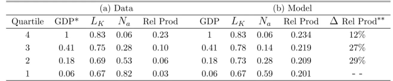
In the previous section we study the evolution of relative productivity along the dynamic transition of a country. In this subsection, we use the model to explain cross-country di¤er-ences in labor productivity. Panel (a) of Table 8 summarizes the cross-country data. The table groups the data for 80 countries, contained in Figure 1, according to income quartiles. For each quartile, it provides median values of 4 variables of interest: GDP per capita, frac-tion of land in capital intensive agriculture, fracfrac-tion of employment in agriculture and of
relative labor productivity between agriculture and non-agricultre.16 In the lower quartiles
of income we observe a smaller fraction of land in the capital intensive sector, a larger share of employment in agriculture and a smaller relative labor productivity than in countries belonging to higher quartiles.
In this subsection, we analyze how much of these cross-country di¤erences can be ex-plained by our model. To this end, we calibrate the model to match the value of the variables
in the highest quartile of the income distribution and set the value of relative prices, PL and
PK; to one. The value of GDP in the other quartiles are obtained by reducing the TFP of
each sector in the same proportion.17
The results of the simulation are shown in Panel (b) of Table 8. The model is calibrated to fully account for cross-country di¤erences in the fraction of land in capital intensive agriculture. The model explains 29% of the di¤erences in relative productivity between countries in the …rst and second quartile, and 27% of di¤erences in relative productivity between countries in the second and third quartiles. In contrast, it explains only 12% of the di¤erences between countries in the two highest quartiles. Therefore, our mechanism explains a larger fraction of relative labor productivity di¤erences when we consider less developed countries. Overall our mechanism explains 17% of the cross-country di¤erences in relative labor productivity.
Notice that our simulation exercise explains only a small fraction of the large di¤erences in the share of employment in agriculture observed in the data. For this reason, the simulation is unable to account for a larger fraction of productivity di¤erences across-countries. However, it is important to note the simulation exercises excludes di¤erences between countries in sectoral productivity that could generate larger di¤erences in both the employment share and the relative productivity. It also excludes cross-country di¤erences in taxes that could result in misallocations that could further contribute to explaining the di¤erences observed in relative labor productivity. These di¤erences in taxes are considered in the following section.
16The data on GDP and relative labor productivity is obtained from Restuccia et al. (2008) and the data
on agricultural employment and fraction of land in the capital intensive sector from the FAO database. All data refers to the year 1985. We compute the median to minimize the e¤ect of outliers.
17We use the calibration of Brazil shown in Table 7 and recalibrate the following parameters c = 0:0051;
= 0:5449; = 0:8536; " = 2:1; AK = 0:1099 and AL= 0:1515, to match PK= PL= 1 and GDP, LK; Na;
and relative productivity in the highest quartile. To match the value of GDP in the third, second, and …rst quartile, we reduce all the sectoral TFPs by factor of 0:5754; 0:3651; 0:2164, respectively.
6
Misallocation of agricultural composition
In this paper, low agricultural labor productivity is explained by less capital stock or lower technology. In contrast, a large part of the literature argues that misallocations of production factors are important to explain low productivity in agriculture. Following this literature, in this section we consider the e¤ect of a permanent increase in the tax rate on the cost of capital
in agriculture, : Changes in this parameter allow us to compare economies with di¤erent
cost of capital. The development literature has shown that development is associated with a reduction in the cost of capital. In particular, Banerjee (2001), Banerjee and Du‡o (2005), Banerjee and Moll (2010) and Karlan (2013) provide evidence showing that the cost of capital is substantially larger in developing countries, specially in agriculture. Therefore, we ask if a permanent reduction in the cost of capital in agriculture can lead to an increase in relative labor productivity.
Figure 10 illustrates the e¤ect of a permanent increase in by comparing the calibrated
economy, in which = 0; with an economy in which = 1: First, an increase in this tax
impoverishes the economy, which causes an income e¤ect that enlarges the agricultural sector and reduces average farm size. These changes are shown in Panels (a) and (b). Panel (c) shows that the relative price of labor to capital intensive crops is lower in the economy with = 1. The price is lower in the initial period because the increase in the cost of the capital is larger in capital intensive agriculture after the tax is introduced, while the reduction that follows is explained by less capital accumulation.
The reduction in the relative price a¤ects agricultural composition. In Panels (d) and (e) it is shown that the fraction of both harvested land and farmers in labor intensive agriculture increase. As a consequence, the agricultural sector as a whole becomes more labor intensive. It is important to note that this e¤ect is increasing during the transition. In the initial period, the fraction of land in labor intensive agriculture increases by about 25%, whereas the increase is 56% in the …nal period.
Panel (f) shows that capital intensity in agriculture relative to non-agriculture declines
after increasing . Since is a tax on capital in agriculture, it directly reduces capital
intensity in both agricultural sectors. The change in agricultural composition, to labor intensive agriculture, causes an additional reduction in the capital intensity of aggregate agriculture.
Finally, the last three panels of Figure 10 illustrate the e¤ect of an increase in on
the relative labor productivity of each agricultural sector and aggregate agriculture. The most striking result is that an increase in the cost of capital has a positive e¤ect on the relative productivity of each agricultural sector, but a negative and sizable e¤ect on the relative productivity in aggregate agriculture. To explain this result, we combine (9) and
the condition de…ning the marginal worker at to rewrite the labor productivity in labor
intensive agriculture in relation to non-agriculture as PL;tYL;t NL;t Yn;t Nn;t = PL;tYL;t NL;t i L;t(at) (1 n) (1 ) :
We next use (17) and (29) to obtain PL;tYL;t NL;t Yn;t Nn;t = L;t a 1 1 s s t NL;t 1 n 1 L L 1 1 :
Finally, using the expression of L;t and the fact that NL;t= F (at) F (at) ; we obtain
PL;tYL;t NL;t Yn;t Nn;t = 1 1 L L ! 1 n 1 L L 1 1 0 B @ 1 at at 1 1 L L 1 at at 1 C A : (31) We follow a similar procedure, using (9) and (29), to rewrite the relative labor productivity in the capital intensive sector as
PK;tYK;t NK;t Yn;t Nn;t = K (1+ )Rt K K xt K (1 ) PK;tAK 1 1 K K K;t NK;t (1 n) (1 ) (1 ) i L;t(at) :
We use (17), the condition de…ning the marginal worker at; the expression of K;t and the
fact that NK;t= 1 F (at) ;to get
PK;tYK;t NK;t Yn;t Nn;t = 1 1 K K ! 1 n 1 K K 1 1 at at 1 1 L L : (32)
From (31) and (32), it is obvious that has no direct e¤ect on the relative labor
produc-tivity in this sectors. It only has an indirect e¤ect through selection, since it a¤ects marginal abilities of farmers in each production sector, as it can be seen in (18) and (19). The intuition
is quite immediate. An increase in reduces the amount of farmers in the capital intensive
sector (atincreases). The remaining farmers have higher abilities, which explains the increase
in the relative productivity of the capital intensive sector. In the labor intensive sector, the number of farmers increases as the economy is poorer. On one hand, low ability individuals
enter this sector (atdeclines), reducing relative productivity. On the other hand, high ability
individuals enter this sector too (at increases), increasing relative productivity. The second
e¤ect predominates in this calibration, which explains the increase in relative productivity.
It follows that relative productivities are a¤ected by indirectly, through changes in the
abilities of the farmers. However, as the numerical simulations illustrate, this e¤ect is small.
In order to explain the positive and large e¤ect of on relative productivity of aggregate
agriculture, we rewrite relative productivity as PL;tYL;t+ PK;tYK;t NL;t+ NK;t Yn;t Nn;t = PL;tYL;t NL;t Yn;t Nn;t NL;t Na;t + PK;tYK;t NK;t Yn;t Nn;t NK;t Na;t (33)
An increase in shifts agricultural composition towards the labor intensive sector, which is
the sector with lower relative labor productive. Therefore, the increase in reduces relative
in is initially small and increasing along the transition. This is a consequence of the e¤ect
of on the sectoral composition, which is also increasing along the transition.
We show that a¤ects relative productivity through changes in the agricultural
compo-sition in Figure 11. In this case, we consider the e¤ect of a permanent increase in when
" = 1: From this exercise, we observe that the increase in reduces the relative price and
the relative capital intensity. However, the price change does not a¤ect agricultural compo-sition (panels (d) and (e) in Figure 11) and, as a consequence, the e¤ect on relative labor
productivity of aggregate agriculture is negligible.18
As we discuss in the introduction, the literature that introduces misallocations to ac-count for cross-ac-country di¤erences in relative productivity, between broad sectors, considers a unique agricultural sector. In this literature, taxes create a wedge between agriculture and non-agriculture that directly a¤ects relative productivity (Restuccia et al., 2008 and Chen,
2017). In our paper, these taxes are given by or . It follows from (31) and (32) that
they directly a¤ect relative productivity. Our contribution to this literature is to show that taxes that do not create this direct wedge between the agriculture and non-agriculture can also a¤ect relative productivity, through agricultural composition. Therefore, in our model,
a reduction in the cost of capital, ; provides an alternative explanation to di¤erences in
relative labor productivity, across countries and time.
The misallocation literature studies di¤erent regulations that limit mobility of workers across sectors or land acquisition. These regulations directly a¤ect the optimal allocation of inputs, mainly in the agricultural sector, which reduces productivity. We show how this type of regulation can a¤ect agricultural composition thus introducing another channel through which relative labor productivity is altered. This is illustrated in Figure 12, where we compare the calibration of Brazil with an economy subject to an extreme labor mobility restriction that prevents workers from moving out of agriculture. This type of restriction is similar to the one introduced in Hayashi and Precott (2008). In this counterfactual economy, the number of farmers remains constant at the level of the initial period. This restriction has three e¤ects. First, it prevents any increase in average farm size, which a¤ects productivity in agriculture negatively, as in Adamopoulos and Restuccia (2014). Second, since the number of farmers is now larger, labor intensive agriculture is bene…ted. This explains the decline in relative prices. As a consequence, farmers and land remain employed in the labor intensive sector. Third, the abundance of farmers and the absence of structural change deter capital accumulation in the agricultural sector. Therefore, relative capital intensity declines. The conjunction of these three e¤ects explains the decline in relative labor productivity. As follows from (33), the reduction in the relative labor productivity is explained by both a reduction in relative productivity in each agricultural sector (see Panels (g) and (h)) and by a process of structural change towards labor intensive agriculture. Therefore, the mechanism introduced in this paper can be seen as complementary to the ones in the misallocation literature in explaining di¤erences in relative labor productivity.
18The increase in impoverishes the economy and as result the number of farmers increases (a
tdeclines).
Given that the fraction of workers remains constant when " = 1, at also declines. This implies that, in this
calibration, farmers with lower ability produce capital intensive crops, which explains the reduction in the relative productivtiy of this sector.
7
Concluding remarks
Di¤erences in labor productivity between developed and developing countries are substan-tially larger in agriculture than in non-agriculture. Since agricultural employment is large in developing countries, the development literature has concluded that explaining these large di¤erences in agricultural productivity is central to understanding cross-country income dif-ferences. We contribute to this literature by showing that the agricultural composition can explain a signi…cant part of low agricultural productivity observed in developing countries.
We use data from the US census of agriculture and FAO to group agricultural products into two agricultural sectors that di¤er only in the capital intensity of the production func-tion. These data is used to calibrate a multisector growth model. We use the model to show that, as the economy develops and capital becomes abundant, the price of labor intensive agriculture relative to capital intensive agriculture increases. This relative price change drives a process of structural change within agriculture that implies: (i) a reduction in the number of farmers, mainly in the labor intensive sector; (ii) an increase in the average farm size; (iii) an increase in the fraction of harvested land used in the capital intensive sector; and (iv) an increase in the capital intensity of the agricultural sector relative to the non-agricultural sector. Since farms are larger and more capital intensive, labor productivity in agriculture increases relative to non-agriculture. We show that these development patterns, implied by our model, are consistent with time series evidence for Brazil and other developing countries, and a cross-country sample that includes developing and developed countries.
In the counterfactual simulations, we show that when structural change within agriculture is limited, by either low substitution of crops in preferences or misallocations of production factors, relative labor productivity is negatively a¤ected.
We use the mechanisms of our model to study how misallocations a¤ect relative labor productivity. To this end, we distinguish between two types of ine¢ ciencies: taxes and regulations. From the development literature, we know that taxes produce a direct wedge between income in agriculture and non-agriculture that a¤ects relative labor productivity. We extend this analysis and show that taxes can a¤ect relative labor productivity indirectly, by altering the composition of agriculture, even without the direct wedge between income in agriculture and non-agriculture. Regarding regulations, we showcase how a policy that limits the mobility of individuals out agriculture misallocates resources within agriculture and reduces the relative labor productivity. In sum, we show that misallocations of factors across agricultural sectors, resulting from di¤erent forms of ine¢ ciencies, can have a negative impact on relative labor productivity.
Finally, throughout this paper, we maintain that the force that drives the process of sectoral composition within agriculture is economic development and capital accumulation. However, we acknowledge that exports of agricultural products could be another potential source of structural change. In the case of Brazil, we have shown that agricultural exports are an important factor since 2000, but trade alone is unlikely to explain the in change agricultural composition observed during the entire period considered.
References
[1] Acemoglu, D., Guerrieri, V. (2008). Capital deepening and nonbalanced economic growth, Journal of Political Economy, 116, 467-498.
[2] Adamopoulos, T. and Restuccia, D. (2014). The size distribution of farms and interna-tional productivity di¤erences, American Economic Review, 104, 1167-1697.
[3] Alvarez-Cuadrado, F., Van Long, N. and Poschke, M. (2017). Capital Labor Substitu-tion, Structural Change and Growth. Theoretical Economics 12, 1229-1266.
[4] Banerjee, A. (2001). Contracting Constraints, Credit Markets, and Economic Devel-opment. In: Dewatripont, M., Hansen, L. and Turnovsky, S. (Eds). Advances in Eco-nomics and Econometrics: Theory and Applications, Eighth World Congress, Volume III, Chapter I, Cambridge University Press.
[5] Banerjee, A. and Du‡o, E. (2005). Growth Theory through the Lens of Development Economics. In Handbook of Economic Growth, Chapter 7, Elsevier.
[6] Banerjee, A. and Moll, B. (2010). Why Does Misallocation Persist?, American Economic Journal: Macroeconomics, 2, 189–206.
[7] Chanda, A. and Dalgaard, C. (2008). Dual economies and international total factor productivity di¤erences: channelling the Impact from institutions, trade, and geography, Economica, 75, 629-661.
[8] Chen, C. (2017). Technology adoption, capital deepening, and international productivity di¤erences, WP 584, University of Toronto.
[9] Chen, C. (2017). Untitled Land, Occupational choice, and agricultural productivity, American Economic Journal: Macroeconomics, 9, 91-121.
[10] Cao, K. and Birchenall, J. (2013). Agricultural productivity, structural change, and economic growth in post-reform China, Journal of Development Economics, 104, 165-180.
[11] Caselli, F. (2015). Accounting for Cross-Country Income Di¤erences, Handbook of Eco-nomic Growth, in: Philippe Aghion & Steven Durlauf (ed.), volume 1, 679-741.
[12] Caunedo, J. and Keller, E. (2016). Capital Obsolescence and Agricultural Productivity, 2016 Meeting Papers 686, Society for Economic Dynamics.
[13] Donovan, K. (2016). Agricultural risk, intermediate inputs, and cross-country produc-tivity di¤erences, mimeo.
[14] Gollin, D., Parente, S., and Rogerson, R. (2002). The role of agriculture in development, American Economic Review, 92, 160-164.
[15] Gollin, D., Parente, S., and Rogerson, R. (2007). The food problem and the evolution of international income levels, Journal of Monetary Economics, 54, 1230–1255.
[16] Gollin, D., Lagakos, D. and Waugh, M. (2013). The agricultural productivity gap, The Quarterly Journal of Economics, 939–993.
[17] Gollin, D., Lagakos, D. and Waugh, M. (2014). Agricultural productivity di¤erences across countries, American Economic Review , 104, 165-170.
[18] Gottlieb, C. and Grobovsek, J. (2019). Communal land and agricultural productivity, Journal of Development Economics, 138, 135-152.
[19] Hayashi, F. and Prescott, E. (2008) . The Depressing E¤ect of Agricultural Institutions on the Prewar Japanese Economy, Journal of Political Economy, 116, 573-632.
[20] Karlan, D., Osei, R., Osei, I. Osei-Akoto and Udry, C. (2014). Agriculture decisions after relaxing credit and risk constraints, The Quarterly Journal of Economics, 129, 597-652.
[21] Kongsamut, P., Rebelo, S., Xie, X. (2001). Beyond balanced growth, Review of Eco-nomic Studies, 68, 869-882.
[22] Larson, D., R. Butzer, Y. Mundlak and Crego, A. (2000). A cross-country database for sector investment and capital, The World Bank Economic Review, 14, 2, 371-391. [23] Lagakos, D. and Waugh, M. (2013). Selection, Agriculture, and Cross-Country
Produc-tivity Di¤erences, American Economic Review, 103, 948-980.
[24] Lucas, R. (1978). On the size distribution of business …rms, The Bell Journal of Eco-nomics, 9, 508-523.
[25] Manuelli, R.E., and Seshadri, A. (2014). Frictionless Technology Di¤usion: The Case of Tractors, American Economic Review, 104, 1368-91.
[26] Ngai, L. R., Pissarides, C. (2007). Structural change in a multisector model of growth, American Economic Review, 97, 429-443.
[27] Restuccia, D. and Santaeulalia-Llopis, R. (2017). Land Misallocation and Productivity, NBER Working Paper No. 23128.
[28] Restuccia, D., Yang, D. and Zhu, X. (2008). Agriculture and aggregate productivity: A quantitative cross-country analysis, Journal of Monetary Economics, 55, 234–250. [29] Valentinyi, Á. and Herrendorf, B. (2008). Measuring factor income shares at the sectoral
level, Review of Economic Dynamics 11, 820-835
[30] Vollrath, D. (2009). How Important are Dual Economy E¤ects for Aggregate Produc-tivity?, Journal of Development Economics, 88, 325–334.
[31] Yang, D. and Zhu, X. (2013). Modernization of agriculture and long-term growth, Jour-nal of Monetary Economics 60, 367–382.