ACOUSTIC LEVITATION SAMPLE-ENVIRONMENT DEVICE FOR BIOPHYSICAL APPLICATIONS

Università degli Studi di Messina

Dipartimento di Scienze Matematiche e Informatiche,

Scienze Fisiche e Scienze della Terra

__________________________

A

COUSTIC

L

EVITATION

S

AMPLE-

E

NVIRONMENT

D

EVICE

FOR

B

IOPHYSICAL

A

PPLICATIONS

Relator:

Prof. Salvatore Magazù

Dr. Antonio Cannuli

A

BSTRACT

The thesis work is mainly focused on issues concerning an acoustic levitation sample-environment device for biophysical applications and the employment of a portable neutron source for biophysical and electronic applications.

Sample preparation and sample-container interaction are critical components for many research investigations. In fact, on the one hand, the reactions between the sample and its container can limit accessibility conditions; on the other hand, heterogeneous container nucleation limits the capacities of “supercooled” liquids or to make over-saturated solutions. In this context, acoustic levitation can be employed for sample preparation as in the case of high concentrated mixtures, starting from solutions.

The aim is to characterize and clarify the physical-chemical mechanisms involved in the formulation processes, the vectorization processes, the stability of the formulations against the stress factors, the associated effects in the presence of bio-protector matrices, characterized by different values of kinematic and thermodynamic fragility, without neglecting the theoretical processes that underlie the acoustic levitation. In this regard, a physical-mathematical model was implemented to study the drying process of a single droplet of solution placed inside a levitator. The aim was to investigate the physical phenomena involved in this process and thus contribute to the general understanding of the drying process in an ultrasonic levitator.

The second thesis section deals with the employ of a portable neutron source, for neutrons activation and detection, is mainly addressed to biophysical and electronic applications. More in detail, the MP320 neutron generator of Thermo Scientific was employed in conjunction with a PINS-GMX

external contact from implanted ions, for INAA (Instrumental Neutron Activation Analysis) investigations. Various simulations have been made with MCNP (Montecarlo N-Particles software) and a special shield has been designed to perform indoor measurements. Main applications of the source, in addition to the aforementioned, are closely related to the other research topics covered such as the field of biomedical, biology, anthropology, nutritional sciences, environmental, history and archaeology, ecology, environmental sciences, materials sciences and as a reference for materials.

T

ABLE OF

C

ONTENTS

ACOUSTIC LEVITATION SAMPLE-ENVIRONMENT DEVICE FOR

BIOPHYSICAL APPLICATIONS………..………...1

INTRODUCTION………..………..…...3

CHAPTER 1: OVERVIEW ON LEVITATION TECHNIQUES…………...8

1.1 Introduction………...2

1.2 Drying processes in an ultrasonic levitator...10

CHAPTER 2: SINGLE-AXIS ACOUSTIC LEVITATOR...17

2.1 Acoustic standing waves………..20

2.2 Mechanical models for motion of an acoustically levitated sphere……….31

2.3 Euler’s equation approach………34

2.4 Surface tension and wettability in complex systems ………..38

2.5 Measurements methods………..….41

INVESTIGATED SAMPLES……….47

1.

Ethylene-Glycol

(Eg)

and

Polyethylene-Glycol

(Peg)

Aqueous

Solutions………...47

2.

Disaccharides Aqueous Solutions: Trehalose, Sucrose and Maltose

Mixtures……….………..53

MATERIALS AND METHODS………..………55

1.

Acoustic Levitator……….………...47

RESULTS AND DISCUSSION………..62

1.

EXPERIMENTAL RESULTS FOR THEORETICAL MODEL TESTING

FOR DISACCHARIDES SOLUTIONS……….………...62

2.

EXPERIMENTAL RESULTS FOR STUDY OF ETHYLENE-GLYCOL

WATER MIXTURES………70

MOTION OF AN ACOUSTICALLY LEVITATED SPHERE…………..75

4.

EXPERIMENTAL RESULTS FOR SURFACE TENSION AND

WETTABILITY IN COMPLEX SYSTEMS……….80

CHAPTER 3: PORTABLE NEUTRON SOURCE...106

3.1 Introduction...62

3.2 Materials and Methods...…...64

3.3 Results and Discussions

CONCLUSIONS………110

REFERENCES………

1

A

COUSTIC

L

EVITATION

S

AMPLE-

E

NVIRONMENT

D

EVICE FOR

B

IOPHYSICAL

A

PPLICATIONS

The thesis work is mainly focused on issues concerning an acoustic levitation sample-environment device for biophysical applications and the employment of a portable neutron source for biophysical and electronic applications.

i)

A

L

The main purpose of this section is to gather a framework of conceptual knowledge on the biophysical processes underlying the formulation processes to develop new protocols for the samples preparation, in particular the structural, dynamic and functional properties were studied, as well as the aggregation, stabilization and protection mechanisms to rationalize the formulation process and to extend their use to a large number of applications in the pharmaceutical, cosmetic, nutritional, cultural heritage and for the study of extremophile organisms.

Sample preparation and sample-container interaction are critical components for many research investigations. In fact, on the one hand, the reactions between the sample and its container can limit accessibility conditions; on the other hand, heterogeneous container nucleation limits the capacities of “supercooled” liquids or to make over-saturated solutions. In this context, acoustic levitation can be employed for sample preparation as in the case of high concentrated mixtures, starting from solutions. Single-axis Acoustic Levitator is shown in Figure 1. The aim is to characterize and clarify the physical-chemical mechanisms involved in the formulation processes, the vectorization processes, the stability of the formulations against the stress factors, the associated effects in the presence of bio-protector matrices, characterized by different values of kinematic and thermodynamic fragility, without neglecting the theoretical processes that underlie the acoustic levitation. In this regard, a physical-mathematical model was implemented to study the drying process of a single droplet of solution placed inside a levitator. The aim was to investigate the physical phenomena involved in this process and thus contribute to the general understanding of the drying process in an ultrasonic levitator. The acoustic levitation technique was implemented to study polymers and disaccharides

2

aqueous solutions, specifically mixtures of water and EthyleneGlycol (EG) and PolyEthyleneGlycol (PEG) with a nominal weight of 200 and 600 Dalton, trehalose, sucrose and maltose; this study also included measurements of surface tension, wettability and density. Such integration approach, in which liquid samples are suspended in the air, by means of an ultrasound field and then analysed by thermodynamic techniques, allowed to follow the drying process as a function of time and to modify the original mixture in a gel-like compound, where extensive chemical cross-linking processes occur. Nowadays, acoustic levitation technique, for the characterization of the structural and dynamical properties of the investigated samples, has been employed in peculiar thermodynamic conditions and in perturbations of a different nature, as in the presence of an electromagnetic field. Furthermore, a study on the development of a prototype that would allow joint, acoustic and electromagnetic levitation is in progress.

Figure 1: Single-axis Acoustic Levitator together with the main characteristics. ii)

P

N

S

The diffusion of electronic devices now reached the most varied fields of application, some of them involve particular operating conditions that require an adequate study of the devices response to external stresses. The electronic components used in the presence of ionizing radiation fields, such as devices used in space applications or in the nuclear field, fall within this field. These last examples are connected by the specificity of the operating conditions, since the devices are subjected to very intense radiation fields. To these application fields, others can be added. For example, can be

3

considered, the power electronics, increasingly widespread in energy applications, which, due to the particular operating conditions, makes the devices used in this field sensitive to the effect of the radiation fields to which they are subject, such as the field of atmospheric radiation. Other examples can be the devices applied in medical applications that involve the use of radiation fields that can significantly compromise the functioning of the associated electronics, such as in nuclear medicine and radiotherapy. In all the cited areas, the gamma and neutron radiations are very important since, being not equipped with charge, they can interact at atomic and nuclear level with the atoms of the crystalline lattice of the materials constituting the devices, with effects that can go from deterioration of the functioning characteristics of the device to the destruction of the same. In this context, at a European and global level, the compact portable systems of neutrons production are of increasing interest. Investigation techniques that employ neutrons as “probe”, able to provide information on the structure of matter, were developed over the years and are constantly increasing. Consequently, the applications of these techniques have also expanded and, today, neutron investigation techniques involve various sectors of research, technological and industrial development. In this second thesis section, the use of a portable neutron source, for neutrons activation and detection, is mainly addressed to biophysical and electronic applications. More in detail, the MP320 neutron generator of Thermo Scientific was employed in conjunction with a PINS-GMX Ortec solid-state photon detector (Figure 2), made with high purity n-type germanium, which allows the entire external contact from implanted ions, for INAA (Instrumental Neutron Activation Analysis) investigations. Various simulations have been made with MCNP (Montecarlo N-Particles software) and a special shield has been designed to perform indoor measurements. Main applications of the source, in addition to the aforementioned, are closely related to the other research topics covered such as the field of biomedical, biology, anthropology, nutritional sciences, environmental, history and archaeology, ecology, environmental sciences, materials sciences and as a reference for materials.

Figure 2: MP320 neutron generator of Thermo Scientific in conjunction with a PINS-GMX Ortec solid-state photon detector.

4

I

NTRODUCTION

In the last years, contactless methods are increasingly employed for the liquid mixtures preparation and experimental investigations; in particular, levitation techniques solve the problems related to container interactions and contamination, furnish a method to study the sample with a very high degree of control.

In general, at high temperatures, reactions with crucibles limit the accessed conditions; while, at lower temperatures, heterogeneous nucleation by containers limits the ability to supercool liquids below their equilibrium melting point or to make supersaturated solutions. The functional behavior and characteristics of cosmetics and pharmaceuticals products depend on their structure. Containerless techniques provide a means of access to supercooled liquids regularly and supersaturated solutions under well-controlled conditions. Using containerless methods enable the synthesis of non-equilibrium forms of materials, often with novel structures.

The word “levitation” derives from the Latin “levitas”, that means lightness and it is the process by which an object is suspended by a physical force against gravity. In particular, acoustic levitation is a phenomenon that allows to move solid objects or liquids in the air, without a contact occurs, taking advantage of the pressure generated by the sound waves and that can be obtained through some physical principles that counteract gravity. More in detail, levitation is a process in which an upward force counteracts downward gravitational force of an object so that there is no physical contact between levitated object and ground.

While at the beginning levitation was claimed by many ancient scholars, such as Isaac Newton, that investigated the possibility of levitation as an opposite force to gravitation, today again some physics investigate several ways of levitation.

Contactless techniques allow to create an opposing force to the gravity to hold the analyzed solution in suspension. Different levitation methods have been studied by, such as optical [2-3], electro-magnetic [4-7], electrostatic [8-11], gas-film [12-14], aerodynamic [15-29] and acoustic levitation [30-51].

5

Optical levitation is generated by an optical trap that is formed by a focused laser beam with an objective lens of high numerical aperture. A dielectric particle will experience a force due to the transfer of momentum from the incident photons.

Electro-magnetic levitation, mostly suitable for electrically conductive materials [1], is generated by a radio-frequency field (≈ 150 kHz), produced by a coil, which induces Foucault currents in the sample. Foucault currents interact with the magnetic field of the coil causing a force that counteracts gravity. This force is proportional to the absorbed power by the sample, as a function of the square of the magnetic field strength and the electrical conductivity of the sample material.

Electro-static levitation is applicable for electrically charged samples which are levitated in an electrostatic field generated between two electrodes. One disadvantage is connected with the experimental setup complexity which hinder its use in combination with many other techniques. It permits to work under vacuum, so to prevent contamination and it also enables to study poor electrical materials with a low melting point.

Gas-film levitation enables the levitation of an object against gravitational force by floating on a thin gas film through a porous membrane. The sample-membrane closeness hampers the use in association with many techniques. It enables to levitate a large amount of material of few grams, that can be also heated thought a furnace.

Aerodynamic levitation, has proved to be a powerful and versatile technique for studying highly reactive liquids. The basic idea is to circulate levitation gas through a nozzle onto the sample from below in order to counteract gravity and lift it above the nozzle. It has the outstanding advantage of supporting any type of material ranging from insulators through semiconductors to metals. The sample can be heated to the desired temperature by means of lasers. Furthermore, the gas flow is regulated and monitored by a mass flow controller enabling to maintain the sample stable for long counting times.

Among these techniques, acoustic levitation has the advantage of not requiring any specific physical properties of the sample, for example a specific electrical charge, a certain refractive index or transparency.

Table 1 reports some distinctive features of levitation techniques as the sample size and weight, the possible processable materials, the required atmosphere and the typical temperature range.

6

Table 1: Distinctive features of levitation techniques: sample size, sample weight, processable materials, required atmosphere and temperature range.

The first use of acoustic levitation dates back to 1933, when Bucks and Muller noticed acoustic fields throughout alcohol mists and droplets [52]. Subsequently, in 1985 Barmatz and Collas developed techniques that used resonant cavities to create regions that can trap small samples [53]. All the described levitation techniques are reported in Figure 1.

Figure 1: Overview on different levitation techniques: i.e. optical, electromagnetic, electrostatic, gas-film, aerodynamic and acoustic levitations.

Levitation techniques sample size sample weight processable materials required atmophere temperature range

Optical ≈ μm ≈ μg conductors and non solids and liquids, conductors

not required not applicable

Electromagnetic 1 – 8 mm up to

Kg

solids and liquids, conductors and non conductors only as function

of frequency as needed (also vacuum if request) limited by material properties Electrostatic 1 – 3 mm up to g

solids and liquids, conductors and non

conductors

as needed (also vacuum if

request)

high, but only for short experiments

Gas film 5 – 50

mm g

solids and liquids, conductors and non

conductors

as needed limited by material properties

Aerodynamic 0,5 – 3,5

mm g

solids, conductors and non

conductors

required up to melting point

Acoustic 0,5 – 3

mm g

solids and liquids, conductors and non

conductors

required limited by material properties

7

C

HAPTER 1

Chapter 1 reports an overview on levitation techniques with a particular reference to acoustic levitation, furthermore drying processes in an ultrasonic levitator are introduced. Finally a specific application for historic cultural heritage conservation.

Recent developments in acoustic levitation and microgravity enable containerless analyses on supercooled liquids and are suitable for investigation of non-equilibrium processes. The current available technology does not allow long experiments with samples larger than a few hundred milligrams, but only to process small samples for very short periods, while acoustic levitation can allow this, because the positioning forces are small and buoyancy-driven convection is eliminated. Acoustic levitation has the advantage of not requiring any specific physical properties of the sample, such as a specific electrical charge, a certain refractive index or transparency.

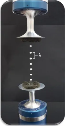
In acoustic levitation, a standing wave is generated by a piezoelectric crystal, which gives rise to a stationary acoustic radiation force [1] when the distance between a transducer and a reflector is an integral multiple of the half wavelength. Is also possible to use two opposed transducers that control the position of the sample by electronically adjusting the acoustic phase. The distance between the two transducers is about 10 wavelengths. Liquid and solid drops, of about 0.5 and 3.5 mm diameter, can be levitated in the vicinity of the pressure nodes; these nodes and anti-nodes appear at fixed points separated by a distance of λ⁄2.

Figure 1.1 shows, in a schematic way, the container-medium-sample interaction mechanisms. The sample can be contaminated by the sample holder, especially at high temperatures (for example chemical reactions increase rapidly with the temperature). Containerless levitation allows the elimination of the extrinsic effects of the heterogeneous nucleation. After a certain time and with a specific power occur equilibrations between the investigated sample and the medium.

8

Figure 1.1: Potential interactions among the investigated sample, the sample holder and the acoustic medium. The sample holder causes contaminations and nucleations in the investigated sample; this latter can evaporate in the acoustic medium after a certain levitation time; at a given power equilibration between the sample and the acoustic medium may occur.

In Figure 1.2a the levitation forces that determine the droplet shape are reported: axial forces are mainly responsible for compensating the gravitational force, while radial forces hold the sample in the pressure node. Figure 1.2b shows a series of images of levitated mixtures drops obtained by varying the frequency of acoustic forces. The drop shape can be compressed by increasing the acoustic forces that can generate an atomization of the drop. Generally, the modulation of the acoustic forces causes oscillations of the drop and, when the stimulation frequency matches the drop resonant frequency, the amplitude of the oscillations becomes very large and this can cause the fall of the drop or its explosion. A further small increase in the acoustic power results in the drop suddenly fragmenting into a mist.

9

Figure 1.2. a) Radial and axial levitation forces. The axial forces (Fz) compensate the gravitational force, while the radial forces (Fr) hold the drop stable in the pressure node. b) Levitated mixtures drops excited by varying the acoustic forces using a sine wave function at different frequencies.

1.1

D

P

U

L

Nowadays, drying processes and evaporation kinetics of levitated droplets are considered complex mechanisms. Although many theoretical models on the drying behavior of suspended droplets have been formulated, only few experimental data are available. Previous investigations often provide only integral information while specific information about the individual physical processes taking place are missing.

In general, levitation [1-5] is a contactless technique that permits to remove sample-holder interplays and decreases contamination in order to study a solution with a high control degree. Among these techniques, acoustic levitation has the advantage of not requiring specific properties of the sample and can treated very small object. It allows obtaining very high concentrations of mixtures starting from solutions, impossible to achieve without the use of levitation. In particular, the importance of acoustic levitation resides in the access to supercooled liquids regularly and supersaturated solutions under well-controlled conditions. Furthermore, the latest updates in acoustic levitation allow container-less studies on supercooled liquids and are fit for analysis of non-equilibrium processes. The present technology assent only to process small samples for very short periods and not long-lasting experiments with samples of a few hundred milligrams; with the acoustic levitation, it is possible thanks to the smallness of the positioning forces and the elimination of the buoyancy-driven convection.

In this context, in acoustic levitation it is fundamental to implement an intuitive model of drying processes occurring when a single droplet is suspended in the air; furthermore, the observation of a single droplet upon drying often enables to track the physical and chemical changes and to get

10

information on the investigated systems. The acoustic levitator is an instrument suitable for the study of droplets kinetics.

Mechanisms of droplet drying are enough complex, in particular they involve a period in which the drying process is constant and it follows the well-known D2-Law, followed by a period where the rate of drying falls.

In general, the evaporation rate of solutions is variable and it follows a non-linear dependence of the square diameter with time. In particular, on levitated droplets evaporation in levitators with strong acoustic fields it was shown that the acoustic streaming in the gas furnishes a convective mechanism bigger than the Stefan flow or natural convection. The acoustic streaming dominates the evaporation process in levitators and in the case of disaccharides aqueous droplets experimental data on D2 (t) were correlated by a linear function reminiscent of the D2-Law.

The D2_{-Law predicts that the square of the droplet diameter decreases linearly with time.}

Few important assumptions must be considered for a droplet in suspension, such as: • heat and mass transfer between liquid and gas phase are diffusion controlled; • a spherical symmetry is considered;

• no radiation effects take place;

• constant and uniform temperature occurs.

The mass flux of vapor leaving the droplet surface can be calculated as: 𝑚̇𝑣 = 𝜋𝐷𝜌𝑣𝑎𝑝𝑜𝑟𝐷𝑔𝑆ℎ (

𝑌𝑣𝑎𝑝,𝑠−𝑌𝑣𝑎𝑝,∞

1−𝑌𝑣𝑎𝑝,∞ ) (1)

where Yvap is the mass fraction at the droplet surface which is supposed to be uniform. The outer

boundary is noted with the subscript ∞ and represents the condition far away from the droplet. The rate change of liquid droplet mass is expressed as follows:

𝑚̇_𝑑 = −𝑑𝑚𝑑 𝑑𝑡 (2)

but 𝑚̇_𝑣 = −𝑚̇_𝑑, so, comparing eqn. (1) with the eqn. (3) the equation for the diameter becomes:

𝜋𝐷𝜌𝑣𝑎𝑝𝑜𝑟𝐷𝑔𝑆ℎ ( 𝑌𝑣𝑎𝑝,𝑠− 𝑌𝑣𝑎𝑝,∞ 1 − 𝑌𝑣𝑎𝑝,∞ ) = −𝜌𝑑𝑟𝑜𝑝𝑙𝑒𝑡 𝜋𝐷 4 𝑑𝐷𝑆2 𝑑𝑡 with 𝐷_𝑆3 = 𝐷_𝑆2∙ 𝐷.

11

Figure 1: Droplet diameter, that can be divided in a constant diameter, that is 𝑫 and in a

variable diameter as function of time, 𝑫_𝑺𝟐.

𝑑𝐷 2 𝑑𝑡 = −4 𝜌𝑔𝑎𝑠 𝜌𝑑𝑟𝑜𝑝𝑙𝑒𝑡𝐷𝑔𝑆ℎ ( 𝑌𝑣𝑎𝑝,𝑠−𝑌𝑣𝑎𝑝,∞ 1−𝑌𝑣𝑎𝑝,∞ ) = −4 𝜌𝑔𝑎𝑠 𝜌𝑑𝑟𝑜𝑝𝑙𝑒𝑡𝐷𝑔𝑆ℎ ln(1 + 𝐵𝑀) (4)

For diffusion-controlled evaporation the film thickness goes into infinity, hence Sh0=2.

The modified Sherwood number Sh takes the value 2 and after substituting the value of Sh0 in eqn.

(1), eqn. (4) becomes: 𝑑𝐷𝑠 2 𝑑𝑡 = −8 𝜌𝑔𝑎𝑠 𝜌𝑑𝑟𝑜𝑝𝑙𝑒𝑡𝐷𝑔ln(1 + 𝐵𝑀) (5) ∫𝑑𝐷𝑠2 𝑑𝑡 𝑑𝑡 = ∫ −8 𝜌𝑔𝑎𝑠 𝜌𝑑𝑟𝑜𝑝𝑙𝑒𝑡𝐷𝑔ln(1 + 𝐵𝑀)𝑑𝑡

in which BM is the Spalding mass transfer coefficient.

The integration of this equation for an initial condition D0, i.e. at t = 0, gives the well-known D2-Law

that describes the temporal evolution of droplet surface of pure liquid:

𝑫𝒔𝟐= 𝑫𝟎𝒔𝟐 − 𝜷𝒕 (6)

where 𝛽 is the evaporation rate coefficient: 𝛽 = 8 𝜌𝑔𝑎𝑠

𝜌𝑑𝑟𝑜𝑝𝑙𝑒𝑡𝐷𝑔ln(1 + 𝐵𝑀) (7)

The density of the liquid droplet is 𝜌_{𝑑𝑟𝑜𝑝𝑙𝑒𝑡}, the density of the gas at the droplet surface is 𝜌_𝑔𝑎𝑠, the diffusion coefficient is 𝐷_𝑔and the Spalding transfer number is 𝐵_𝑀.

In addition to the evaporation rate, another important parameter in droplet evaporation is the lifetime of the droplet, also called evaporation time τend, which can be determined from eqn. (6) with

𝐷|_{𝑡=𝜏𝑒𝑛𝑑} = 0:

𝜏𝑒𝑛𝑑 = 𝐷02

12

C

HAPTER 2

In acoustic levitation a standing wave is generated by a piezoelectric crystal which gives rise to a stationary acoustic radiation force. In Physics Education, acoustic levitation furnishes an effective and straightforward method to localize the nodes of acoustic standing waves and to highlight some interesting physical phenomenologies. In Chapter 2 two mechanical models to study the damped oscillations of an acoustically levitated sphere are introduced and a method to determine surfece tension in complex systems. The work is addressed to graduate Physics, Engineering and Mathematics students.

One of the primary subjects of Physics is the concept of waves. Waves are perturbations originated from a source which, although of different nature, have in common the same characteristic equation. The property of the waves to be superimposed gives rise, among other things, to the phenomenon of non homogeneous distribution of their energy in space.

Transverse waves are those in which the oscillation occurs in a direction perpendicular to that in which the wave propagates.

In longitudinal waves the oscillation of the medium are parallel to the direction of propagation, as shown in Figure 2.1.

In gases, such as air, only longitudinal waves propagate, since cohesion effects able to recall the medium towards the equilibrium position are negligible. It should be noticed that, the particles that constitute the medium do not translate but oscillate around their equilibrium position. A wave, therefore, in a strict sense, does not involve the transfer of matter.

In the following the attention will be addressed only to the longitudinal waves and, in particular, to standing acoustic waves that propagate inside an acoustic levitator. It will be shown how particles

13

immersed in acoustic waves are influenced by forces that can be schematized by means of mechanical models constituted by a mass-spring system and by a stretched string.

Figure 2.1. Longitudinal wave in which the oscillations of the medium consist of compressions and rarefactions that occur in the same direction in which the wave propagates.

It should be stressed that in most undergraduate and graduate Physics Education courses, students are usually introduced to the concept of standing waves by means of a discussion on the transverse standing waves on a string. In fact, static images of the standing waves on a fixed string are more easily understood because they show wave patterns corresponding to the transverse displacement of the string.

However, acoustic waves are longitudinal waves and the particle motion associated to a standing acoustic wave, for example in a pipe, is directed back and forth along the pipe axis. In this context, acoustic levitation furnishes an effective and straightforward method to visually show the nodes of acoustic standing waves whose positions are stationary.

14

Figure 2.2. Drawing of the Kundt’s tube apparatus (denoted inside Figure 2.2, as Figure 6 and Figure 7) and the powder patterns created by it (denoted inside Figure 2, as Figures 1, 2, 3 and 4).

Despite standing wave levitation phenomena were first observed in Kundt’s tube experiment [1], the first use of acoustic levitation dates back to 1933 [2]. Subsequently, in 1985 Barmatz and Collas developed techniques that used resonant cavities to create regions that can trap small samples [3]. Figure 2.2 shows a drawing of the Kundt’s tube (denoted inside Figure 2.2, as Figure 6 and Figure 7) and the powder patterns created by it (denoted inside Figure 2.2, Figures 1, 2, 3 and 4) [1]. This experimental apparatus allows the measurement of the sound speed in a gas or a solid rod and it was invented in 1866 by a German physicist August Kundt. It is used today only for demonstrating standing waves and acoustical forces.

15

In the last years, many levitation techniques [4] have been developed by scientists, for example optical [5-6], electro-magnetic [7-10], electrostatic [11-13], gas-film [14-15], aerodynamic [16-29] and acoustic levitation [30-55].

In many cases levitation is a contactless technique that permits to remove sample-holder interplays and to decrease contamination; furthermore, acoustic levitation is employed for obtaining high concentrations of mixtures starting from solutions. Electric levitation for example is achievable with conductive materials. For these reasons acoustic levitation is widely used in biophysics both for the investigation of aqueous solutions [56-59], disaccharides [60-85], proteins [86-93], polymers [94-138], polyols [139-145], nano-materials [146-148] and systems of biotechnological interest [149-150]. In particular acoustic levitation is more and more employed in the preparation of highly concentrated mixtures and in conjunction with spectroscopic techniques [151-156].

In this paper, an approach to explain standing waves by means of an acoustic levitator is presented. In particular, it is possible to visually show the nodes of the acoustic standing wave whose positions are stationary; furthermore, two mechanical models to study the damped oscillations of a suspended particle [157-162] are reported, showing as acoustic levitation allows to explain the physical principle of standing waves in an intuitive way.

2.1

A

S

W

Waves obey to the same differential equation and it is this property that allows to give a unified description. In general, considering a perturbation represented by a function 𝑓 = 𝑓(𝑥, 𝑡), the wave equation is: 𝜕2𝑓 𝜕𝑥2

=

(1)

where 𝑥 is the position, 𝑣 the velocity of the wave and 𝑡 the time.

This is a differential equation to partial derivatives, linear of the second order. Solutions of eq. (1) can be written in the form:

𝑓 = 𝑓(𝑥 ± 𝑣𝑡)

(2)

It is relatively simple to prove that eq. (2) is solution of eq. (1), introducing the intermediate variable 𝑠 = 𝑥 ± 𝑣𝑡. It follows that: 𝜕𝑓 𝜕𝑥

=

=

;

=

= ±𝑣

.

(3)

16

Observing that the derivatives of the function 𝑓 respect to 𝑥 and 𝑡 are obtained by multiplying the derivative respect to 𝑠, for 1 and for ±𝑣, it is possible to write:

𝜕2𝑓 𝜕𝑥2

=

;

= 𝑣

.

(4)

Substituting eq. (4) in eq. (1) it is possible to verify that eq. (1) is verified.

The two solutions, 𝑓(𝑥 − 𝑣𝑡) and 𝑓(𝑥 ± 𝑣𝑡), describe respectively a wave that propagates in the direction of the 𝑥 axis and in the opposite direction to that of 𝑥 axis.

A particular case of relevant interest is that in which the source that generates the wave oscillates of harmonic motion, with a fixed pulsation 𝜔. The argument of the wave function must therefore contain, in addition to 𝑥 and 𝑡, also the pulsation 𝜔; dimensional considerations suggest to express the function in the form:

𝑓 = 𝐴𝑐𝑜𝑠(𝑘𝑥 ± 𝜔𝑡) or 𝑓 = 𝐴𝑠𝑖𝑛(𝑘𝑥 ± 𝜔𝑡)

(5)

in which the argument of the trigonometric functions is called “phase.” It is easy to verify that both these functions are solution of eq. (1), as long as exists the relationship:

𝑘 =

𝜈

(6)

The parameter 𝑘 is called “wave number.”

The following relationships are easily verifiable: 𝑣 =𝜆

𝑇= 𝜆𝜈 𝜔

𝑘 and 𝜔 = 2𝜋

𝑇 = 2𝜋𝜈.

The phenomenon called “standing waves” occurs when two waves of the same nature and of the same frequency propagate in the same medium in opposite directions and they overlap.

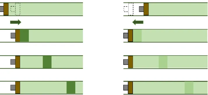
Sound is a longitudinal pressure wave, constituted by the alternation of compressed and rarefied air layers. Considering a long tube, full of air, closed at one end by a piston that can slide back and forth. As the piston advances, it compresses the volume of air adjacent to it; consequently, the air pressure contained in that volume increases and the air tends to expand from both sides, compressing the next volume of air and at the same time restoring the previous pressure from the piston side; in this way the impulse produced by the piston is transmitted along the tube (see Figure 3).

If the piston moves in the opposite direction a pressure vacuum is created.

Figure 4 shows what happens to a sphere volume at different times, as a rightward-traveling wave passes by. The darker regions indicate higher pressure and density zones, whereas the lighter regions indicate lower pressure and density zones.

17

In the 1st case, the sphere volume is located at its equilibrium position (indicated by the vertical blue line) moving towards the right side with maximum velocity; at this position the pressure and density take the maximum value too while the net force is zero. In the 2nd case, the sphere volume is decelerating due to the pressure which is higher on the right than on the left particle side. In the 3rd case, the sphere value is at its maximum displacement and acceleration, while its velocity is zero. In the 4rd case it is moving leftward while in the 5rd case, it crosses the equilibrium position with the maximum negative velocity.

Figure 2.3. Longitudinal pressure wave, constituted by the alternation of compressed and rarefied air layers, represented by a long tube, full of air, closed at one end by a piston that can slide back and forth.

Figure 2.4. Half cycle of a sphere volume at a few different times, as a rightward-traveling wave passes by.

18

For an acoustic wave, intensity is defined as the energy carried by the wave per unit area and per unit of time.

The human ear can be considered as a sensitive receiver with the ability to perceive sounds whose intensity varies in a large interval. Ear response has a particular non-linear characteristic curve; it does not produce a double sound sensation when it doubles the objective intensity of the pressure wave, but has a logarithmic response. The ear response also depends on the sound frequency as shown in Figure 2.5. Each of the graph curves refers to sounds of different frequencies that generate the same sound sensation. The set of all isophonic curves defines the field of audibility.

Acoustic waves which can be perceived by the human ear have a frequency between 20 Hz and 20 KHz; below 20 Hz the waves are called “infrasonic” and above the 20 KHz “ultrasonic” (see Figure 5). The lower curve refers to the threshold of audibility, the highest one indicates the pain threshold (loudness level), at the frequency of 1000 Hz; they correspond respectively to 10-12 _W/m2 _{and 1 W/m}2_.

Figure 2.5. Field of audibility (upward). Sound range diagram (below), from infrasounds to ultrasounds. Acoustic waves perceived by human ear span, with a different weight, from 20 Hz to 20 KHz.

19

Figure 2.6. Intensity of a sound wave 𝑰 that pass through a surface 𝑨 = 𝟏 𝒎𝟐_.

The intensity of a sound wave 𝐼 is the energy that it carries in the unity of time through a surface of 1 m2 placed perpendicular to the direction of propagation of the wave (see Figure 2.6).

It is therefore a power per unit of surface and its measure unit is W/m2:

𝐼 =

∆𝑡∙𝐴

=

𝑃

𝐴

(7)

This definition adapts to any type of wave; from it derives an important property of the energy transmission through the waves. It is such as a small sound source that emits with the same intensity in all directions (isotropic source) and it considers the energy that flows inside a pyramid that has as vertex the source (see Figure 2.7).

From the definition of 𝐼follows: 𝐼₁ = 𝑃

𝐴1 = 𝑃 𝑙₁2 and 𝐼2 = 𝑃 𝐴2 = 𝑃

𝑙₂2 from which it derives: 𝐼2

𝐼1 =

𝑙22

𝑙₁2.

Figure 2.7 shows that the triangles of vertex 𝑂 and basis 𝑙₁ and 𝑙₂ are similar, so derives that: 𝑙1

𝑙2 =

𝑑1

𝑑2.

Substituting it in the previous equation it is possible to obtain: 𝐼2

𝐼1 =

𝑑12

𝑑22 that is the inverse square law

20

Figure 2.7. Wave propagation follows the inverse square law of distance.

Figure 2.8. Standing waves in an acoustic levitator which furnish stable equilibrium locations for levitated particles.

21

Therefore, the wave intensity, emitted by an isotropic source, decreases with the inverse of the square of the distance from the source.

When an acoustic wave reflects off of a surface, the interaction between its compressions and rarefactions induces interferences, that can combine to create a standing wave. Standing acoustic waves have defined nodes, i.e., areas of minimum pressure, and antinodes, i.e., areas of maximum pressure. Figure 2.8 shows the stable equilibrium locations for levitated particles.

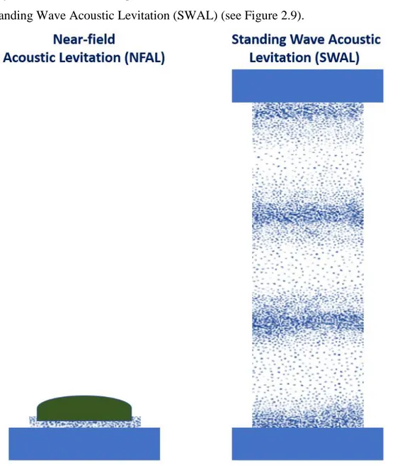
Two different kinds of waves are employed in acoustic levitation to generate acoustic radiation pressure, they are defined as traveling waves or Near-field Acoustic Levitation (NFAL) and standing waves or Standing Wave Acoustic Levitation (SWAL) (see Figure 2.9).

Figure 2.9. Two different kinds of waves are employed in acoustic levitation to generate acoustic radiation pressure: traveling waves or Near-field Acoustic Levitation (NFAL) (on the left) and standing waves or Standing Wave Acoustic Levitation (SWAL) (on the right).

The first ones propagate through a medium with transport of energy, the second are stationary waves, generated by two traveling waves, an incident and a reflected wave. They present pressure nodes, i.e.,

22

positions where the pressure is zero and antinodes, in which the pressure fluctuates between a maximum and minimum value.

In NFAL, samples are levitated and transported at a very small distance above a vibrating surface using ultrasonic Surface Acoustic Waves (SAW)s by means of squeeze film effects in near field. In SWAL, small samples of different shape are levitated in pressure nodes. The acoustic radiation force limits the sample weight. A typical SWAL design, which has one transducer and one reflector, creates a standing wave as shown in Figure 2.10, where the acoustic radiation pressure balances the gravity.

Waves, produced by a transducer and a reflector present pressure nodes and anti-nodes along the blue vertical line. A sample is trapped at a pressure node because of the time-averaged forces of the acoustic radiation pressure. These forces at pressure antinodes push the object axially. The sample is located slightly below a pressure node due the gravitational force. In Figure 2.11, a representation of the acoustic force, the pressure wave and the acoustic potential is reported. The period of the pressure wave is the twice of that of the acoustic force wave.

23

Figure 2.11. a) Sketch of the acoustic force (solid red line) and the pressure wave (dashed blue line) and b) the acoustic potential (solid orange line).

In an acoustic levitator, a standing wave is generated by a piezoelectric crystal which gives rise to a stationary acoustic radiation force when the distance between two transducers is an integral multiple of the half wavelength.

The transducers, made of aluminium alloy, are driven by piezoelectric drivers, inside an aluminium mounting tubes of 38 mm diameter. The nominal frequency of the transducers is 22 KHz. The distance of the two transducers is set to a nominal separation of 10 acoustic wavelengths, approximatively 150 mm. Two acoustic absorbing foam disks approximately 50 mm in diameter are glued onto the face of the transducer horns to reduce unwanted reflections that can cause instabilities in the levitated sample. For a perfect gas, the equation of state, known as ideal gas law, is:

𝑃𝑉 = 𝑛𝑅𝑇

(8)

In an adiabatic process, pressure 𝑃 is a function of density 𝜌:

𝑃 = 𝐶𝜌

(9)

where 𝐶 is a constant.

Pressure and density can be divided into mean and total components: 𝐶 =𝜕𝑃

𝜕𝜌:

𝑃 − 𝑃

= (

𝜕𝜌

) (𝜌 − 𝜌

)

(10)

The adiabatic bulk modulus for a fluid is defined as:

𝐵 = 𝜌

(

𝜕𝜌

)

(11)

24

𝑃 − 𝑃

= 𝐵 (

𝜌0

)

(12)

Condensation, 𝑠, is defined as the change in density for a given ambient fluid density.

𝑠 =

𝜌₀

(13)

The linearized equation of state becomes: 𝑝 = 𝐵𝑠, where 𝑝 is the acoustic pressure (𝑃 − 𝑃0).

The continuity equation for the conservation of mass is:

𝜕𝑃

𝜕𝑡

+

𝜕

𝜕𝑥

(𝜌𝑢) = 0

(14)

where 𝑢 is the flow velocity of the fluid. The equation can be linearized and the parameters can be divided into mean and variable components, as following:

𝜕

𝜕𝑡

(𝜌

+ 𝜌

𝑠) +

𝜕

𝜕𝑥

(𝜌

𝑢 + 𝜌

𝑠𝑢) = 0

(15)

Considering that ambient density changes with neither time nor position and that the condensation multiplied by the velocity is a very small number:

𝜕𝑠

𝜕𝑡

+

𝜕

𝜕𝑥

𝑢 = 0

(16)

Euler's force equation for the conservation of momentum is:

𝜌

𝐷𝑡

+

𝜕𝑃

𝜕𝑥

= 0

(17)

where 𝐷 𝐷𝑡⁄ is the convective, substantial or material derivative. From the linearization of the variables:

(𝜌

+ 𝜌

𝑠) + (

+ 𝑢

) 𝑢 +

(𝑃

+ 𝑝) = 0

(18)

Neglecting small terms, the equation becomes:

𝜌

𝜕𝑡

+

𝜕𝑝

𝜕𝑥

= 0

(19)

Considering the time derivative of the continuity equation and the spatial derivative of the force equation results in:

𝜕2𝑠

𝜕𝑡2

+

𝜕2𝑢

25

𝜌

𝜕𝑥𝜕𝑡

+

𝜕2𝑝

𝜕𝑥2

= 0

(21)

and multiplying the first by 𝜌₀, subtracting the two and substituting the linearized equation of state, it becomes:

−

+

= 0

(22)

The result is:

𝜕2𝑝 𝜕𝑥2

−

= 0

(23)

0 is is the speed of propagation.

The solution of eq. (22), can be found as:

𝑝 = 𝑝

sin (𝑘𝑥)𝑒

(24)

where 𝑝₀ is the pressure amplitude, 𝑘 = 𝜔 𝑐⁄ the wave number, 𝜔 the angular frequency and a ₀ pressure node located at 𝑥 = 0 is the boundary condition.

Spheres of different diameter and weight, can levitate in the pressure nodes; these nodes and anti-nodes appear at fixed points separated by a distance of λ⁄2. Knowing the frequency of the transducer, 𝑓 = 22𝐾𝐻𝑧 and the velocity sound, 𝑣𝑠 = 343 𝑚 𝑠⁄ at the considered temperature 𝑇 = 22°𝐶, it is

possible to determine the wavelength of the standing wave as it follows:

𝜆 =

𝑓

=

343000

22000

= 1,56𝑐𝑚

(25)

In Figure 12, the forces that are responsible for compensating the gravitational force and that hold the sample in the pressure node, are sketched.

Figure 12. Levitation forces that are responsible for compensating the gravitational force and that are able to levitate the particle.

26

An object in the presence of a sound field will experience forces associated with the field. An acoustic force arises from the scattering of the sound wave by the body. In order to have an object suspended in the acoustic field, the acoustic force should counteract the gravity force, i.e., weight of the object.

2.2

M

M

M

A

L

S

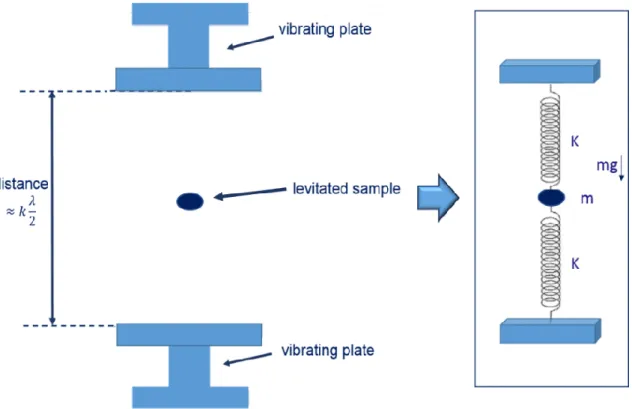
Two mechanical models will be introduced to study the damped oscillations and the motion of an acoustically levitated sphere around the node. They represent respectively longitudinal and transverse forces and are constituted by a mass-spring system and by a stretched string.

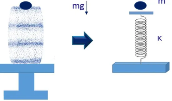
In principle, an acoustic levitator is a system in which a transducer produces an impulse, characterized by a wave-form that permits to a sample to levitate, but in unstable condition. It can be dealt as a mechanical equivalent model, constituted by a mass-spring system of elastic constant k, connected to a mass m (see Figure 2.13).

Figure 2.13. Mass-spring system of elastic constant k to study the damped oscillations of a mass around a node (longitudinal forces).

27

Figure 2.14. Mass-spring system of elastic constant 𝟐𝒌 to study the damped oscillations of a

mass around a node.

A mechanical model to study the damped oscillations of a mass around a node is constituted by two springs of equal elastic constant 𝑘, connected to the mass 𝑚 and is shown in Figure 2.14.

The system can be simplified in a single mass-spring system of elastic constant 2k. The equation of the system is the following second-degree differential equation:

𝑚𝑦̈ + +γ

𝑦̇ + 2𝑘𝑥 = −𝑚𝑔

(26)

in which 𝑚 is the mass, γ_𝐿 the longitudinal damping coefficient, 𝑘 the elastic constant, 𝑔 the gravity acceleration, F = −mg the force weight, 𝑦 describes the position, 𝑦̇ and ÿ are respectively the first and second derivate of 𝑦.

The solution of the equation is constituted by the sum of a solution in 𝑡, 𝑦_ℎ(𝑡) and a particular solution, 𝑦𝑝:

𝑦

(𝑡) = 𝐴

𝑒

𝑠𝑖𝑛(𝜔𝑡 + 𝜑)

𝑦

= −

2𝑘

with 𝜔_𝐿 = √2𝑘

𝑚 pulse or angular frequency, measured in [rad/s].

28

𝑦(𝑡) = 𝐴

𝑒

𝑠𝑖𝑛(𝜔𝑡 + 𝜑) −

2𝑘

(27)

The second mechanical model is employed to study the damped oscillations of a mass around the node (transverse forces, as shown in Figure 2.15.

Figure 2.15. Stretched string to study the damped oscillations of a mass around a node.

Considering a mass 𝑚, connected to two equal stretched strings of length 𝐿, on which a tension 𝑇 acts. If the mass is moved of a small step x in the horizontal direction, assuming that the tension 𝑇 not varies appreciably, it is possible to obtain that the recall force is equal to: 𝐹 = − (2𝑇

𝐿) 𝑥.

So, the equation of the system became in this case: 𝑚𝑥̈ + +γ_𝑇𝑥̇ + (2𝑇

𝐿) 𝑥 = 0 (28)

in which 𝑚 is the mass, γ𝑇 the transverse damping coefficient, 𝑘 the elastic constant, 𝑇 the tension

on the two stretched strings, 𝐿 the length, 𝑥 describes the position, 𝑥̇ and ẍ are respectively the first and second derivate of 𝑥. The solution of eq. (28) is:

𝑥

(𝑡) = 𝐴

𝑒

𝑠𝑖𝑛(𝜔𝑡 + 𝜑)

₍₂₉₎

where for the pulsation is: 𝜔_𝑇 = √2𝑇

29

2.3

E

E

A

Standing wave levitation approach takes in account a model which assumes enough small, incompressible and rigid sphere levitating in presence of acoustic standing wave. For fluid it assumes that effect of viscosity can be neglected and that barotropic relation p = f (ρ) holds. Because of our assumptions we can use Euler’s equation:

𝜕𝑣⃗

𝜕𝑡+ (𝑣 ∙ ∇)𝑣 = − ∇p

𝜌 (1)

assuming that the flow of fluid is irrotational, it is possible to express vector of velocity with gradient of scalar function ɸ (velocity potential): 𝑣 = ∇ɸ. Continuity equation holds:

𝜕𝜌

𝜕𝑡+ ∇ ∙ (𝜌𝑣 ) = 0 (2)

which can be written as:

1

𝜌 𝜕𝜌

𝜕𝑡 = ∇

2_{ɸ (3)}

For a medium, such as air, in which from barotropic relation follows 𝑑𝑝

𝑑𝜌 = 𝑓

′_{(𝜌) = 𝑐𝑜𝑛𝑠𝑡 = 𝑐}2

differential equation for ɸ exact to first order leads to wave equation for ɸ: ∇2_{ɸ =} 1

𝑐2

𝜕2ɸ

𝜕𝑡2. (4)

Eq. (1) can be written as

∇ɸ̇ = ∇ (∫𝑑𝑝

𝜌)

̇

(5) from which follows non-stationary Bernoulli equation:

ɸ̇ − ∫𝑑𝑝_𝜌 = 𝑣2

2. (6)

For further derivation of integral ∫𝑑𝑝_𝜌 we expand barotropic relation into series in terms of factor 𝑠 =

𝜌−𝜌0 𝜌0 : 𝑝 = 𝑓(𝜌₀− 𝑠𝜌₀) ≈ 𝑓(𝜌0) + 𝑠𝜌0𝑓′(𝜌0) + 1 2𝑠 2_𝜌 02𝑓′′(𝜌0) + ⋯ (7)

From this expansion we can express dp and combine it with expression 𝜌−1≈ 𝜌₀−1(1 − 𝑠 + 𝑠2_{− ⋯ ).}

30 𝛿𝑝 = 𝑝 − 𝑝₀ = 𝜌₀𝜕ɸ 𝜕𝑡+ 𝜌0 2𝑐2( 𝜕ɸ 𝜕𝑡) 2 −1 2𝜌0𝑣 2_{. (8)}

To get solutions for pressure variation it is need to calculate velocity potential from wave eq. (4). For that we need to take into consideration boundary conditions which of course sharply depend on geometry of the levitated object. Solution for ɸ from (4) will be oscillatory. For small spheres equality ɸ = |ɸ| cos(𝑘ℎ) cos (𝜔𝑡) can be shown (h denotes position of levitated particle in z-direction). From definition of velocity potential and Bernoulli equation (6) it follows that pressure variation will also oscillate along distance between sound radiator and levitated object. It can be shown that force on enough small-levitated particle created in travelling waves is smaller for few orders of magnitude (𝐹 ∝ 𝑟_𝑠6_{) than force created in stationary waves. This is why effect of travelling waves can be}

neglected. Acoustic force on a small, rigid sphere (model described before) in a standing wave is derived to be:

𝐹 = 8𝜋𝑟𝑠2(𝑘𝑟𝑠)𝐸̅𝑠𝑖𝑛(2𝑘ℎ)𝑓 ( 𝜌0

𝜌𝑠). (9)

It is expressed with wave number k, radius of sphere rs, mean total energy-density of sound in a

medium 𝐸̅ =1

2𝜌0𝑘

2_{|ɸ|, density of sphere ρ}

s and so called relative density factor 𝑓 which in case for

stationary wave is defined as

𝑓 (𝜌0 𝜌𝑠) = 1+2₃(1−𝜌0 𝜌𝑠) 2+𝜌0 𝜌𝑠 . (10)

Another different approach to derive force on small particle in standing wave field is with acoustic potential. The acoustic force is obtained from

𝐹 = −∇𝑈. (11)

Expression for acoustic force, like (9), is of course the same, regardless which approach we use. Acoustic potential is often expressed in form

𝑈 = 2𝜋𝑟𝑠[𝑓1 〈𝑝₀2_〉 3𝜌0𝑐2− 𝑓2 𝜌0 2 〈𝑣0 2_{〉] (12)}

with 〈𝑣₀2〉 and 〈𝑝₀2_{〉 being time-averaged square of velocity and pressure of the acoustic wave, both}

considered in the point where levitated object is found. 𝑓₁ (monopole coefficient) and 𝑓₂ (dipole coefficient) are numerical factors given by

𝑓₁ = 1 −𝜌0𝑐02

𝜌𝑠𝑐𝑠2 (13)

and

𝑓₂ = 2(𝜌0−𝜌𝑠)

31

where again index 0 presents surroundings (medium) and index s particle (sphere). Eq. (12) can be presented with maybe more intuitive form:

𝑈 = 𝑉𝑠[𝑓1〈𝐸𝑝𝑜𝑡〉 − 3

2𝑓2〈𝐸𝑘𝑖𝑛〉] (15)

with 𝑉_𝑠 as volume of a sphere and 〈𝐸_𝑝𝑜𝑡〉 =_2𝜌1

0𝑐2〈𝑝0

2_{〉 and 〈𝐸} 𝑘𝑖𝑛〉 =

𝜌0

2 〈𝑣0

2_{〉 being averaged potential}

(of compressed medium) and kinetic (due motion of medium) energy density of acoustic wave. Particle‘s equilibrium points are at 𝐹_𝑖 = 𝜕𝑈

𝜕𝑥𝑖 = 0. Acoustic force according to (11) depends on

geometry of a chamber in which experiment is performed. With definition of acoustic potential (11) we can see that particle‘s tendency to minimal force can be seen as tendency to potential minima. In presence of gravity, gravitational term has to be added to expression for acoustic potential (into (12) or (15)): 𝑈 = 𝑈𝑎𝑐𝑜𝑢𝑠𝑡𝑖𝑐+ 𝑈𝑔𝑟𝑎𝑣 where gravitational contribution is defined as

𝑈𝑔𝑟𝑎𝑣 = (𝑚𝑠 − 𝑚0)𝑔ℎ (16)

where ms and mf are the mass of the sample and the mass of fluid, which is displaced because of

presence of particle whereas h again denotes vertical position of particle.

By now viscosity of medium was neglected. This approximation is justified when there is no presence of rigid boundary in medium and wave attenuation is neglected. Otherwise viscous term 𝜂∇2𝑣 has to be added to Euler‘s eq. (1).

Because of viscosity acoustic attenuation is emerged, in other words, momentum of acoustic waves is transferred to the medium, resulting in net displacement of it (i.e. acoustic streaming) in space between boundaries. This net displacement creates gradient of streaming velocity and viscous force which acts as holding force. Hence, levitated object is considered stabilized.

Experimentally it was noticed that this streaming velocity is proportional to amplitude of sound radiator, by increasing amplitude, streaming velocity (and viscous force) also increases. In standing waves levitation, system different corrections are considered. Thickness of viscous boundary layer is defined as:

𝛿 = √_𝜌2𝜂

0𝜔 (17)

Expressed with η as coefficient of viscosity and ω frequency of sound. In standing wave levitation effect of viscosity can be neglected as long distances within a few δ are not reached. It can also be neglected for particles for which characteristic dimension exceeds characteristic dimension of viscous boudary layer (rs >> δ). Since we consider model which assumes particles with rs << δ we have to regard viscous corrections.

Viscous corrections can be presented with numerical factors f1 and f2. Since viscosity does not affect

32 𝑓₂ = (𝜌0 𝜌𝑠, 𝛿 𝑟𝑠) = 𝑓2(𝜌̃, 𝛿̃) = 2(1−𝛾(𝛿̃))(𝜌̃−1) 2𝜌̃+1+3𝛾(𝛿̃) (18) with factor 𝛾(𝛿̃) = −3

2(1 + 𝑖(1 + 𝛿̃))𝛿̃ and taking only 𝑅𝑒𝑓2(𝜌̃, 𝛿̃) in eq. (12). Contribution of

viscous corrections depend on viscosity of medium, material of lifted particle and its diameter. Acoustic levitation by standing wave has been employed for several different techniques. Main advantage of this approach is the fact that levitated object is isolated and it can not react with its surroundings any more. This is very desirable when studying or dealing with chemical reactions especially with the fact that levitated particle is easy reachable and available for handling. In physics isolating of sample is desirable when observing phase transitions, process of crystallization or to study the structure of proteins or nanoparticles. Similar use of standing wave levitation is in interesting experiment to isolate droplets of liquid and observe their evaporation process by illuminating droplet and determining its volume with help of shadows.

2.4

S

T

W

C

S

Wettability is the feature of a solid to prefer to be in contact with one fluid rather than another and it describes the balance between adhesive and cohesive forces.

In a liquid, cohesive forces avoid contact with the surface, forming a spherical shape when all three phases, i.e. solid, liquid and gaseous, are in equilibrium, whereas between the liquid and the solid surface, adhesive forces cause the liquid to spread across the surface. If a surface of a material is attracted to a certain liquid, it is considered “-philic” for that substance; while a surface that tends to repel a certain liquid, is considered “-phobic”.

Liquids possess different important properties like density, viscosity and surface tension; the latter is the only property thanks to which a solid having greater density than that of a liquid can float on to the surface of the liquid. Also the shapes of the drop are governed by the property of surface tension. More specifically, the surface tension value depends by the purity of certain liquids. Liquids are distinguished from gases, because they exhibit a free separation surface, that acts like a stretched thin membrane and possesses certain mechanical properties due to cohesion between molecules.

The property to show the tendency of contracting and then that force acting on the surface of a liquid and that tends to minimize the surface area it affects physical properties such as wettability, is defined surface tension.

In this framework, the conjunction use of acoustic levitation and InfraRed (IR) spectrocopy offers a valid approach to determine the surface tension value. It is fundamental to isolate a single drop suspended in the air and to observe the physical and chemical changes. Furthermore, it allows

33

obtaining very high concentrations of mixtures starting from solutions, impossible to achieve without the use of levitation.

In a liquid, the drop shape is ideally determined by surface tension; each molecule is pushed equally in all direction by neighboring molecules, then the resulting force is equal to zero. Unlike internal molecules of the bulk, the superficial molecules not present neighboring molecules in every direction to provide a balanced net force, but they are pushed inward by the neighboring molecules, creating an internal pressure, as showed in Figure 1a. So the liquid voluntarily contracts its surface area to maintain the lowest surface free energy.

Figure 2.16. Molecules in a liquid a) Molecules in a zoom of a liquid drop, in which the surface tension is determined by the unbalanced forces of liquid molecules at the surface; b) a molecule in a liquid is surrounded on sides by other molecules that attract it equally in all directions with a net force equal to a zero; c) a molecule in the surface suffers a net force toward the interior, due to the absence of molecules above this surface; d) cross section of a primitive three-dimensional model of a molecule interfacing to vacuum.

More specifically, as showed in the below part of Figure 2.16, it is considered a molecule in a liquid, surrounded on sides by other molecules that attract the central molecule equally in all directions with a net force equal to a zero (Figure 2.16b), a molecule in the surface (Figure 2.16c) and a cubic grid, in which the molecules are located, with length equal to the molecular separation length, i.e. 𝐿_𝑚𝑜𝑙.

34

In Figure 2.16c, the absence of molecules above the surface, causes a net attractive force toward the interior. This force causes the liquid surface to contract toward the interior until repulsive collisional forces from the other molecules stop the contraction at the point in which the surface area is a minimum. If the liquid is not influenced by external forces, the sample forms a sphere, with minimum surface area for a given volume.

From a mathematical point of view, looking at figure 1d, each molecule has six bonds to its neighbours in the interior, while only five on surface, for which considering a total binding energy 𝜀 of a molecule,a surface molecule is linked for 5

6𝜀. The missing binding energy corresponds to adding

an extra positive energy1

6𝜀for each surface molecule, therefore the binding energy can be calculated

as 𝜀 ≈ ℎ ∙ 𝑚, where ℎ is the specific heat of evaporation and 𝑚 = 𝑀_𝑚𝑜𝑙⁄𝑁_𝐴 = 𝜌𝐿3_𝑚𝑜𝑙 the mass of a single molecule, in which 𝑀_𝑚𝑜𝑙 is the molecular mass, 𝑁_𝐴 the Avogadro's number and 𝜌 the density. Dividing the molecular surface energy 1

6𝜀 with the molecular

area scale 𝐿2_𝑚𝑜𝑙, it is possible to obtain the surface energy density or surface tension 𝛾:

𝛾 ≈ 1 6𝜀 𝐿_𝑚𝑜𝑙2 ≈ 1 6 ℎ∙𝑚 𝐿2_𝑚𝑜𝑙≈ 1 6ℎ ∙ 𝜌 ∙ 𝐿𝑚𝑜𝑙 (1)

where𝜌𝐿_𝑚𝑜𝑙 is the effective surface mass density of a layer of thickness 𝐿_𝑚𝑜𝑙.

The apparatus, shown in Figure 2.17, is employed to furnish a simpler definition of surface tension.

Figure 2.17. C-shaped wire frame, employed to furnish a simpler definition of surface tension. It is constituted by a frame on which is placed a wire that can slide with negligible friction, containing a thin film of liquid and can be employed to measure the surface tension of a liquid.

35

It is constituted by a C-shaped wire frame on which is placed a wire that can slide with negligible friction, containing a thin film of liquid. It can be also employed to measure the surface tension of a liquid. From this example, it is possible to notice how it is necessary a force ℱ to move the slider to the right and extend the liquid surface that is contracted because of the surface tension.

This surface tension (γ), measured in 𝑁 ∙ 𝑚−1_{= 𝐽 ∙ 𝑚}−2_{, can be defined as the force ℱ per unit of}

length over which it acts, as expressed in the following equation: 𝛾 =ℱ

𝐿 (2)

𝐿 = 2ℓ is a total length, where ℓ is the length of the slider and ℱ acting force.

From a general point of view, the sign of 𝛾 depends on the strength of the cohesive forces holding molecules of a sample together compared to the strength of the adhesive forces between the opposing molecules of the interfacing samples.

If the surface tension of two liquids is negative, a large amount of energy can be released by maximizing the area of the interface, so the two fluids are mixed thoroughly instead of being kept separate. An example is that of alcohol and water. Immiscible fluids, such as oil and water present instead a positive surface tension that makes them seek towards minimal interface area with maximal smoothness.

2.5

M

M

STALAGMOMETRIC METHOD

Different measurement methods for surface tension determination are generally employed, the most common is the stalagmometric method. It consists in the measurement of weight of several liquid drops that leak out of the glass capillary of a stalagmometer (Figure 2.18). If the weight of each drop is known, it is also possible to count the drops number which leaked out for the surface tension measurement. The drops are formed slowly at the tip of the glass capillary placed in a vertical position; the pendant drop at the tip starts to break away when its weight reaches that value balancing the surface tension of the liquid.