Alma Mater Studiorum – Università di Bologna
Anno Accademico 2016 - 2017
SCUOLA DI SCIENZE
Dipartimento di Chimica Industriale “Toso Montanari”
Corso di Laurea Magistrale in
Chimica Industriale
Classe LM-71 - Scienze e Tecnologie della Chimica Industriale
Obtainment of chitosan with different
molecular weight by varying chitin
decarbonation conditions and study of a
mathematical model representing the
process
Tesi di Laurea sperimentale
CANDIDATO Matteo Verdolini
RELATORE Prof. Daniele Caretti
CORRELATORE
3
Abstract
The effects of different chitin decarbonation conditions on chitosan molecular weight have been studied. The factors that could affect chitosan molecular weight and that have been studied in this work are temperature, time and hydrochloric acid concentration; the factor that proved to mostly affect the chitosan molecular weight is the temperature, followed by time and acid concentration. The effect of chitin molecular weight on the finally obtained deacetylation degree has also been studied, and proved to be almost irrelevant. The effect on chitosan molecular weight given by deacetylation carried out with different NaOH concentration has been analyzed; this factor proved to give inversely proportional effect on chitosan molecular weight.
Riassunto
Sono stati studiati gli effetti delle diverse condizioni di decarbonatazione della chitina sul peso molecolare del chitosano così ottenuto. I fattori che possono influire di più sul peso molecolare del chitosano e che sono stati studiati sono temperatura, tempo e concentrazione di acido cloridrico; il fattore che è risultato essere più influente sul peso molecolare è la temperatura, seguita da tempo e concentrazione di acido. E’ stato inoltre studiato l’effetto del peso molecolare della chitina sul suo grado di deacetilazione ottenuto alla fine del processo, ed è risultato essere praticamente irrilevante. E’ stato analizzato l’effetto di diverse concentrazioni di NaOH utilizzate durante il processo di deacetilazione sul peso molecolare del chitosano; questo fattore ha provato di avere un effetto inversamente proporzionale sul peso molecolare.
4
Index
Abstract ... 3
Riassunto... 3
1 Introduction ... 7
1.1 Procambarus Clarkii (American Red Crab) ... 7
1.1.1 Description ... 7
1.1.2 Environmental Problem ... 8
1.1.3 Composition of the exoskeleton ... 9
1.2 Chitin and Chitosan ... 11
1.2.1 Description ... 11
1.2.2 Properties and applications of chitin, chitosan and chitosan oligosaccharides (COS) ... 12
1.2.2.a Chitooligosaccharides ... 13
1.2.3.b Application of COS in food industry ... 14
1.2.3.c Application of COS-based systems as carriers of anticancer drugs 14 1.2.3.d Other industrial applications ... 16
1.3 Chitosan obtainment methods ... 17
1.3.1 Deproteinization... 17
1.3.1.a Enzymatic Deproteinization ... 19
1.3.1.b Chemical Deproteinization ... 20
b.1 Acid Hydrolysis ... 21
b.2 Basic Hydrolysis ... 23
1.3.2 Demineralization and its effect on molecular weight ... 24
1.3.3 Deacetylation ... 25
1.4 Determination of deacetylation degree... 26
5
1.4.2 Determination of DD using NMR ... 27
1.5 Determination of molecular weight of a polymer ... 28
1.5.1 GPC ... 28
1.5.2 Molecular weight through viscosity ... 30
1.5.2.a Capillary viscometers ... 30
1.5.2.b Types of viscosity ... 31
1.5.2.c Determination of intrinsic viscosity and molecular weight ... 33
1.5.2.d Other ways to determine [𝜼]: the Fedors equation ... 36
2 Aim of the project ... 37
3 Results and discussion ... 39
3.1 Response surface methodology ... 39
3.1.1 Design of experiment: general notes on the Central Composite Design ... 40
3.1.1.a Preliminary study: Determination of upper and lower limits ... 42
Acid concentration ... 42
Temperature ... 44
Time ... 44
2.1.1.b Design of Experiment ... 45
2.1.2 Determination of the mathematical model ... 46
Method of least squares ... 47
Optimization ... 48
3.2 Analysis of the results ... 49
3.2.1 Collection of the data ... 49
3.2.2 Analysis of the first response: Kinematic Viscosity ... 51
ECHIP analysis of kinematic viscosity ... 52
3.2.3 Determination of intrinsic viscosity (to be used for MW determination) ... 54
6
3.2.3.a Intrinsic viscosity using Kraemer viscosity plot: analysis of the results
... 55
ECHIP analysis of intrinsic viscosity obtained from inherent viscosity ... 56
3.2.3.b Intrinsic viscosity using Fedors equation: analysis of the results ... 58
Determination of the Fedors coefficient cm ... 59
ECHIP7 analysis of intrinsic viscosity obtained from the Fedors equation .. 61
3.3 Determination of the molecular weight ... 62
3.3.1 Determination of coefficients K and α ... 62
3.3.2 ECHIP7 analysis of molecular weight ... 63
3.4 Effect of molecular weight of chitin on the deacetylation degree ... 67
3.5 Effect of deacetylation conditions on molecular weight ... 71
4 Conclusions ... 73 5 Experimental part ... 75 5.1 General Notes ... 75 5.2 Raw Material ... 75 5.3 Washing ... 77 5.4 Deproteinization ... 79 5.5 Decarbonation ... 81 5.6 Deacetylation ... 83
5.7 Measurement of flowing times for viscosimetry ... 85
7
1 Introduction
The approach to this work of thesis comes from the necessity to deal with the economical and environmental problem that the red crab of the swamps of Guadalquivir is generating as an invader species.
The invasion of this species is fought using the massive capture of this crab; this has generated a proliferation of little-small factories whose purpose is the treatment of this crab finalized to the obtainment of direct-consumption food from its abdomen. These treatments generate a big amount of solid residuals, which are mostly heads and shells of these crabs.
The solution to the problem consists in a conversion of these residuals in a high added-value product, which is the chitin, or its derivative, chitosan. Nowadays the mentioned production of chitin is estimated around 1011 tons/year1, and the exoskeletons of these crabs represent the most important source of raw material.
1.1 Procambarus Clarkii (American Red Crab)
1.1.1 Description
The Procambarus Clarkii is a crustacean of the family of the cambaridae, with a cylindric-shaped body. The exoskeleton of the adults is dark red but some are coffee-colored. The young ones are instead grey, with some black shapes.
It lives in many kinds of freshwater: rivers, plantations, irrigation canals ecc., avoiding strong-current rivers; it’s very territorial and aggressive towards his owns species.
It’s benthic and omnivorous, it usually eats insects, larvas, debris, preferring though animal matter.2
8
Figure 1.1 – Picture of the Procambarus Clarkii
1.1.2 Environmental Problem
Until the second half of the last century the native river crab (Austropotamobius
pallipes), was widely spread in the water streams of the andalucian limestone
mountains and in the rest of the national territory.
Since then, the Spanish economical dinamization has been causing an industrialization of the country, bringing harmful effects to the aquatic environments, like water contamination, shores alteration or destruction of the fluvial geomorphology, which bring a sort of decline of the associated communities.
In 1974, with economical purpose, the American Procambarus clarkia was introduced in the swamps of Guadalquivir. Given their debris-eater nature, these crabs are modeler of most of the fluvial communities, in which can be found bryophytes, macrophytes, macro-invertebrates, amphibious and fishes. Without any doubt, they are a key-species for the energy-fluxes of the environment, but they caused a lot of trouble.
In first place, given its voraciousness and reproductive capacity, the Procambarus managed to send away the native crabs from their original and environmental nest. Second, its introduction put the native crab in a risky situation. The crab plague named afanomicosis (derivating from a fungus, the Aphanomyces astaci) came together with the American crab to the Iberian Peninsula; this disease causes a 100% mortality of the affected native population, and this brought almost to the extinction of the species in just 30 years.
9 So that we can definitely say that the red crab is a concerning environmental problem.3
Furthermore, the growth of the American red crab causes economical losses to the rice cultivations, very common in this region.
To stop, or slow down this diseases caused by the crabs, factories working and producing food from them were born. This originated a second environmental problem, which is the generation of a solid residual, the exoskeleton of the crab, which is the great part of its body weight.
1.1.3 Composition of the exoskeleton
To take advantage of any residual it is important to know its chemical-physical properties and composition. The nature of the residual is very variable, but the concentration results are very often between typical values.
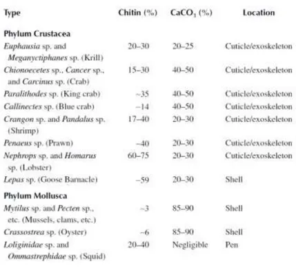
The exoskeleton is usually formed of 30-40% of proteins, 30-50% of calcic carbonate and 20-30% of chitin. At lower concentrations there are the lipid-pigments which give to the crab the typical red color.4
The exoskeleton is formed by an external epicuticle, followed by an exocuticle, an endocuticle and the internal layer of the epidermis. This is common between both marine and terrestrial organisms, so there could be differences in concentrations of chitin, carbonates, and proteins depending on the exoskeleton zone and the species.
A list of commercially exploited marine species and their chitin and calcium carbonate content is shown in Table 1.1.
10
Table 1.1 - List of commercially exploited marine species and their chitin and calcium carbonate content
In the cuticle we can find two different types of chitin, one is tubular (stick-shaped) and other is laminar, binded to two different types of proteins.4 The chitin locates itself in layer-shapes, and its principal purpose is to serve as organic matrix for structural stabilization (structural fibers).
A schematic interpretation of this organic matrix is reported in Figure 1.25
11
1.2 Chitin and Chitosan
1.2.1 Description
The chitin is a polysaccharide widely spread in nature, in fact is the second most abundant polymer after cellulose.
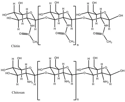
Chitin is a cationic amino polysaccharide composed of N-acetyl-d-glucosamine (GlcNAc, 2-acetamido-2-deoxy-d-glucose) with β (14) glycosidic bonds between each monomer.
When chitin reaches a nitrogen content of more than 7% by weight, or when the degree of deacetylation (DD) is over 60% the term “chitosan” is preferred.
In nature, chitin is found 90-95% acetylated.
Figure 1.3 - Molecular structure of chitin and chitosan
Chitin occurs in three polymorphic solid state forms designated as α, β and γ chitin which differ in their degree of hydration, size of unit cell, and number of chitin chains per unit cells.
12
Figure 1.4 – Polymorphic solid states of chitin
In the α-chitin the chains of polysaccharide are disposed like sheets, all oriented in the same direction, they are grouped as orthorhombic compact cells.6 In the β-chitin the chains are disposed in anti-parallel way, grouped as monoclinic cells. The third structure can be considered as the combination of the previous ones, as the chains are oriented two in one direction, and the third in the opposite direction.7 The most common polymorph in nature is the α-chitin, which for this reason has been more studied than the other two.
1.2.2 Properties and applications of chitin, chitosan and chitosan oligosaccharides (COS)
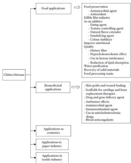
Both chitin and chitosan have unusual multifunctional properties, including high tensile strength, bioactivity, biodegradability8, biocompatibility, nonantigenicity, and nontoxicity4, which made them possible to be used in many applications. Furthermore, the chemical modifications of the three reactive functional groups of chitosan have increased the applications of chitosan in different fields (Figure 1.5).9
13
Figure 1.5 – Most exploited applications of chitosan
1.2.2.a Chitooligosaccharides
Even though chitin and chitosan have various properties that enable them to be applied in many fields, their poor solubility at neutral pH due to high molecular weight and high viscosity limit their application at certain industries, especially in the food and biomedical fields.
However, chitosan oligosaccharides (COS), which are composed of 2-10 units of d-glucosamine units are readily soluble in water. This is due to the short chain lengths and the presence of free amino groups in the d-glucose units.10
This greater solubility of COS at neutral pH has attracted attention for the application of COS in different fields where poor solubility of chitin and chitosan has been a limiting factor.
14
1.2.3.b Application of COS in food industry
The main utilization of chitosan in the food industry is the food preservation. The microbial deterioration and oxidation of foods are the major problems that arise in the increasing of the shelf life of foods. However, food preservation has been achieved successfully with the chemical preservatives. The growing consumer demand toward foods without chemical preservatives has received attention due to natural products, including chitin, chitosan, and COS. The special properties such as antimicrobial activity and antioxidative activity allow the chitin, chitosan and especially COS to get successful as natural preservatives in the food industry.
Different microorganisms, including bacteria, fungi and yeast, are responsible for the microbial deterioration of foods and they act as food pathogens as well. Though chitosan also exhibits antimicrobial property, the greater efficiency of the COS against the microorganism and greater solubility increase the possibilities of COS to be applied as a natural food preservative. The COS can act against both bacteria and fungi that are involved in the spoilage of food. However, scientists have found that the antibacterial activity of the COS is higher, compared to their antifungal activity.11
1.2.3.c Application of COS-based systems as carriers of anticancer drugs The principal modes of cancer management are surgery, radiotherapy, and chemotherapy. Recently hormonal therapy and immunotherapy are increasingly being used as well, but their applications are limited for a few cancer types such as breast neoplasia.12 Chemotherapy, the use of cytotoxic drugs to kill cancerous cells, remains the most common approach for cancer treatment. Generally, cytotoxic drugs are highly toxic but poorly specific, and do not differentiate between normal and cancer cells. Therefore, conventional chemotherapy administration or systemic administration has been shown to produce side effects.
15 Most of the drug content is released soon after administration, causing drug levels in the body to rise rapidly, peak, and then decline sharply, leading to unacceptable side effects at the peaks and inadequate therapy at the troughs.13 Due to the short duration of action, repeated injections are often required, which can lead to the exacerbation of side effects and inconvenience, and can unfortunately lead to less patient compliance. In systemic administration, cytotoxic drugs are extensively transported to the whole body, therefore, only a small fraction of the drugs reach the tumor site and other healthy organs or tissues can be affected or damaged by the nonspecific action of the cytotoxic agents.12
Due to this obstacles, controlled or localized release technology has been replacing systemic administration and has some potential for cancer treatment. For its antibacterial, biocompatible, biodegradable and anticancer activity, therapeutic applications of chitosan nanoparticles possessing mucoadhesive properties, has been widely studied and formulated in anticancer drug delivery systems.
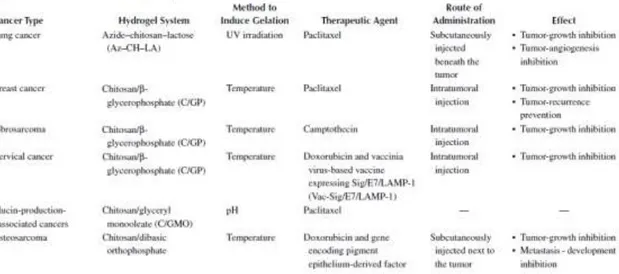
One of the solutions which use chitosan-based systems for drug delivery is the use of in situ injectable chitosan hydrogels for localized and controlled release of therapeutics. Sustained-release injectable formulations are basically designed as microparticulates (microcapsules or microspheres), implants, or gel systems.14 Drugs are commonly loaded into microspheres via a passive absorbtion method whereby microspheres are added to drug solution. Microspheres swell in solution and the drug molecules enter the gel matrix.15 However, the efficiency of this loading method for cytotoxic drugs in limited and a high loading capacity is unattainable. An implant requires surgery to insert it near the tumor site, which adds to the cost and the risk of this system. These problems have oriented research towards injectable in situ gelling formulations.16 Injectable in situ chitosan hydrogels that have been trialed in the treatments of cancers are summarized in Table 1.2.17
16
Table 1.2 – Some of the injectable in situ chitosan hydrogels already trialed
1.2.3.d Other industrial applications
Here are other industrial fields where the chitosan production is strongly implanted: - Clarification, prevention of the oxidation, stabilization of color and antibacterial agent in wine. Chitosan has a good affinity with the phenolic molecules, which are the main responsible of the oxidation and dimming of wine. It also reduces the quantity of polyphenols and stabilizes the white wine in the same way an already widely utilized compound like the potassium caseinate does. Thanks to its antibacterial ability, it is also used to eliminate the microorganisms responsible of the degradations of vines, like the bacteria Brettanomyces.
- Purification of water effluents. Chitosan can be used as a tool to purify residual waters thanks to its high absorption ability. Other feature of the chitosan, which can be useful in water purification, is its flocculating ability.
- Deacidification of drinks such as fruit juices or coffee. To this purpose, it is common to use chitosan salts in which the amino group acts as a weak base.
17
1.3 Chitosan obtainment methods
Industrial techniques for chitin and chitosan extraction from different shell waste normally rely on harsh chemical processes which generate large quantities of hazardous chemical wastes. In spite of that, several procedures for the preparation of chitin and chitosan from different shellfish wastes have been developed over the years, some of which form the basis of the chemical processes used for the industrial production of chitin and derivatives.18
Schematically, the exoskeleton of the P. Clarkii is composed by an organic matrix made of chitin which, as said before, is a polymer having a structural purpose. Bonded to it there are proteins of different nature and an inorganic phase made by calcium and magnesium carbonate, which confers toughness and mechanical resistance to the exoskeleton.
Therefore, the production of chitosan from chitin requires the elimination of the proteins and the inorganic phase and, at last, the deacetylation to obtain chitosan.
1.3.1 Deproteinization
The deproteinization consists of the elimination of the proteins bonded to the chitin. The nature of the chitin-protein bond is vary, and there are many models describing this interaction.
Hackman, using iontophoresis and paper chromatography, determined in 1960 the presence of aspartic acid, histidine and D-Glucosamine. This allowed him to conclude that there was a peptide bond between a non-acetylated amine group of the chitin and a carboxylic group of the protein-chain (Figure 1.6)
18
Figure 1.6 – Hackman’s model of chitin-protein bond
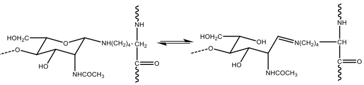
Another model proposed by Hackman is the union between the chitin and the protein through the formation of a Schiff base, with a terminal unit N-acetylglucasamine 2-acetamide-2-deoxy-D-glucose of the chitin (Figure 1.7)
Figure 1.7 - Another Hackman’s model of chitin-protein bond
Hunt, in the early 1970 determined that the protein-chitin complex can be explained with two structures formed by two actual amino acids: the N-glycosidic structure involving the amino group of the asparagine and the O-glycosidic structure involving the serine (respectively left and right structure in Figure 1.8).
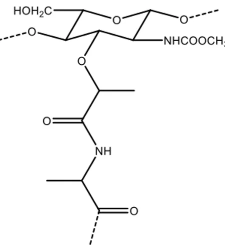
19 Rudall and Kenchington formulated another possible complex chitin-protein, through the carboxylic group of the N-acetylmuramic acid and the amino group of a terminal alanine (Figure 1.9).
Figure 1.9 – Rudall’s and Kenchington’s model for the complex chitin-protein
So, as it is shown, many forms of chitin-proteins interactions are speculated; this implies that it is necessary to apply a method which can eliminate proteins independently from the nature of their bond with the chitin, to make sure that the deproteinization is effective.
Generally, there are many methods to achieve this deproteinization, but they can be assorted in two groups: chemical deproteinization and enzymatic deproteinization.19
1.3.1.a Enzymatic Deproteinization
Thanks to the advancements in biochemistry and, most of all, to the advances in chemical engineering, enzymes are being incorporated more and more in the industrial processes, and not only in the agro-alimentary industry, where fermentation processes are performed.
An example is the incorporation of enzymes in the deproteinization for chitin production. There are several enzymes which could be used in order to achieve the deproteinization of the exoskeleton of crustaceans, like for example the
20
proteinase SV1 (Manni, Ghorbel-Bellaaj, Jellouoli, Younes, & Nasri, 2010), where the reaction was achieved at pH of 8.0, temperature of 40°C and for 3 hours, accomplishing to diminish the protein percentage from 40,83±1,22% to 10,78±0,2%.
Other enzymes used for the deproteinization were derived from tuna, papaya and other extracted from some bacteria.20
A problem related to this kind of deproteinization, comparing it to the more traditional chemical deproteinization, are the too long reactiontime, the lower effectiveness and the proteic residual naturally associated to the process.21
The efficiency in the deproteinization of the exoskeleton of crabs of different commercial enzymes: Delvolase®, Cytolase PCL5®, Econase CEPi®, Econase MP
1000®, MaxameTM MNP® and Ccllupulin MG®, was compared getting to the
conclusion that the Delvolase® is the most effective enzyme. It managed to
eliminate almost 90% of proteins, after a one-day incubation.22
1.3.1.b Chemical Deproteinization
Hackman and Goldberg used different extraction conditions, each of them was associated to a different kind of chitin-protein interaction.23
Water at pH 7 for 48 hours for non-bonded water-soluble proteins.
Sodium sulfate 0,17M at pH 7 for 48 hours for proteins connected with weak bonds like Van der Waals forces.
Urea 7M at pH 7 for 48 hours, for proteins bonded with H-bonds.
NaOH 0,01M at Tamb for 5 hours, for proteins bonded with electrostatic forces.
NaOH 1M at 50-60°C for 5 hours, for proteins connected with covalent bonds.
Proteins linked to the chitin with electrostatic bonds like Van der Waals forces or hydrogen bonds loose their bounding ability varying the pH of the solution;
21 because protoning or de-protoning functional groups makes the protein change its nature.
The proteins linked through covalent bonds are almost 5% of the proteins of the exoskeleton, furthermore they are the most difficult to remove because of the bond strength. The main connection between the chitin and the protein is the peptide bond between a non-carbonated amino group of the chitin and a terminal carboxylic group of the protein. This bond is stable in water, but can be broken by heating or using strong acids or basis through hydrolysis. This hydrolysis is nothing else than an acyl nucleophilic substitution, giving an amine and a carboxylic acid. In an acid medium the amine will be protonated as ion ammonium, in a basic medium the carboxylic acid will be deprotonated as ion carboxylate.
The mechanism of the hydrolysis of an amide is very similar to the mechanism of the hydrolysis of the other carboxylic derivatives.
b.1 Acid Hydrolysis
The hydrolysis in acidic medium goes through two steps: the formation of a tetrahedric intermediate and its successive dissociation. To make the nucleophilic attack possible, the carboxylic oxygen must be protonated, so that the amide results activated. The cation produced in this step is stabilized by resonance.
Once the amide gets O-protonated, the nucleophilic addition of the water happens:
22
The next step is the formation of the ion ammonium with the protonation of the nitrogen:
After that, the dissociation of the ion happens, giving ammonia and the protoned form of the carboxylic acid:
Since we are in acid medium, the most stable species are the ammonium ion and the carboxylic acid. The equilibrium constant of the last step is so high that makes the global reaction irreversible:
23 b.2 Basic Hydrolysis
Like for the acid hydrolysis, this process happens in two steps: the formation of a tetrahedric intermediate and its dissociation giving the breaking of the amide bond. In alkaline medium, the hydroxyl ion carries out a nucleophilic attack to the carbonyl group of the amide, to give the anionic form of the tetrahedric intermediate.
In aqueous medium, the anion interacts with water, deprotoning it to give the neutral species of the tetrahedric intermediate.
In the next step the protonation of the intermediate is accomplished. As opposed to the acid hydrolysis where the most stable form was the O-protonated form, the most stable species here is the N-protonated form.
This latter species suffer from an attack of a basis, promoting the hydrolysis of the amide bond, and giving the carboxylic acid and the corresponding amine.
24
Of course, this species is not stable in an alkaline solution, so the carboxylate ion irreversibly forms. This latter is so stable in basic medium, that makes the global reaction irreversible.23
1.3.2 Demineralization and its effect on molecular weight
This step consists of the elimination of inorganic phase of the exoskeleton. The removal of calcium carbonate (approximatively 95% of the inorganic matter), calcium phosphate, and other mineral salts found in shells is accomplished by extraction with dilute acids. It has been shown to be important that the amount of acid is stoichiometrically equal to or greater than all the minerals present in the shells to ensure complete demineralization.24
Most of the authors coincide about the utilization of hydrochloric acid as reactant for this step, as it is a cheap and easily available acid.
The reaction of elimination of the calcic carbonate with hydrochloric acid is the following:
CaCO3 + 2HCl H2O + CO2(g) + CaCl2
It is generally agreed that the processing conditions strongly affect the molecular weight and DA of chitin. Although HCl may be the cause of detrimental effects on the intrinsic properties of the purified chitin, it remains the most commonly used decalcifying agent in both laboratory and industrial scale production of chitin. As a rule, as the acidic conditions for demineralization (pH, time, and temperature) become harsher, the molecular weight of the products thus obtained becomes lower. Indeed, chitin is an acid-sensitive material and can be degraded by several pathways: hydrolytic depolymerization, deacetylation, and heat degradation leading to physical property modifications.25
25 Anyway, as it was said before speaking about COS, also the low molecular weight chitosan may be used for many application, so it surely could be interesting to explore different routes and conditions which can lead to a lower molecular weight polymer as well.
1.3.3 Deacetylation
Chitin can be converted to its N-deacetylated product, i.e., chitosan, by homogeneous or heterogeneous alkaline N-deacetylation. The degree of deacetylation (DD, %) is defined as the ratio of N-deacetylated (amino) groups to
N-acetyl groups at the C2 position in the backbone.26
When chitin reaches a nitrogen content of more than 7% by weight, or when the degree of deacetylation (DD) is over 60% the term chitosan is preferred.
Chitin and/or chitosan has several distinctive biological properties depending on their deacetylation degree, including biocompatibility and biodegradability, cellular binding capability, acceleration of wound healing, hemostatic properties, and anti-bacterial properties.26
The degree of deacetylation is defined as the molar fraction of
N-acetylglucosamine units in the chain:
DD = 100 ∗ 𝑛𝐺𝑙𝑐𝑁
𝑛𝐺𝑙𝑐𝑁+ 𝑛𝐺𝑙𝑐𝑁𝐴𝑐
where, nGlcN is the average number of D-glucosamine units and nGlcNAc is the average number of N-acetylglucosamine units.
26
1.4 Determination of deacetylation degree
Several methods for determining the degree of deacetylation have been elaborated, from simple, such as pH-metric titration, UV-Vis spectroscopy, infrared spectroscopy, elemental analysis, to complex ones, which require complex and expensive equipment, such as 1H-NMR spectroscopy and 13C-NMR spectroscopy. Anyway, the most common analytical methods for the determination of DD of chitosan are the FTIR (Fourier Transform Infrared Spectroscopy) and NMR (Nuclear Magnetic Resonance, mostly 13C-NMR and 1H-NMR).
1.4.1 Determination of DD using FTIR
Infrared (IR) spectroscopy is widely used because of its simplicity and rapidity, it is non-destructive and it is not necessary dissolve the sample; however, other problems associated with spectroscopic techniques, such as broadening of a peak and overlapping of two or more peaks which leads to incorrect results, are often detected. This technique is appropriate for qualitative study; when quantitative analysis is performed, it is necessary to carry out some complex procedures, such as statistical analysis of several absorption ratios.
Different approaches have been described by Kasaai27 to calculate the DD. One of them consists of the evaluation of the absorbance ratio of the probe band (determination of the N-acetyl or amine content) and the absorbance of a reference band; the intensity of this band does not vary with the DD. The DD of an unknown sample can be calculated by comparing the value of the ratio with similar ratio of samples with known DD. Determination of DD can also be performed based on linear calibration plots of the absorption ratio of chitin or chitosan samples with a known DD against their DD. The DD of the unknown samples was determined from the equation of the calibration curve.
27
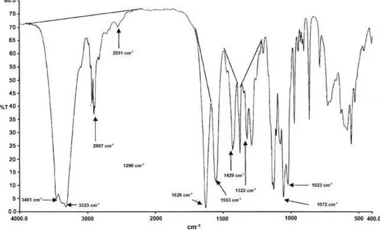
Figure 1.10 - A typical spectrum of N-acetyl d-glucosamine showing the positions of probe and reference bands and corresponding baselines27
1.4.2 Determination of DD using NMR
For quantitative analysis, NMR spectroscopy either liquid-state 1H-NMR for soluble samples or solid-state 13C-NMR is the preferred method because of its simplicity, quickness, and accuracy, at least in solution. Moreover, the American Standard Test Method organization has selected the 1H-NMR as the standard method for the determination the DD in chitosan samples.27,28 In case of 13C-NMR spectroscopy, although it is not necessary to dissolve the samples, it is essential that the samples are highly pure to obtain suitable spectrum.29
Fernández Cervera et al. used the solid-state 13C-NMR to estimate the DD of chitosans obtained from lobster chitin. The calculation was performed according the equation DD = ICH3/IC1 + IC2 + IC3 + IC4 + IC5 + IC6/6, where (IC1; IC2; IC3; IC4; IC5;
IC6) are the relative intensities of the resonance of the ring carbon and (I CH3) is the methyl carbon obtained by 13C-NMR.29
Abdou30 applied the 1H-NMR spectroscopy to determine the DD of chitosan samples obtained from different sources. Samples were dissolved in D2O
acidified with DCL to improve solubility. The 1H-NMR spectra of chitosan showed the characteristic signals: the peak at 4.9 ppm that corresponds to C1 proton of
28
glucosamine unit in chitosan, the peaks at 3–4 ppm that correspond to C2–C6 protons of glucosamine and N-acetylglucosamine units; the peak at 2.06 ppm that corresponds to amide methyl protons and at 2.21 ppm for acetic acid moiety. The DD was calculated according to the method of Lavertu31:
DD(%) = [1 − 1 3 𝑥𝐼𝐶𝐻3 1 6 𝑥 𝐼(𝐻2−𝐻6) ] ∗ 100
1.5 Determination of molecular weight of a polymer
Analytic techniques for the determination of molecular weight can be broken down into secondary (or relative) and primary (or absolute) techniques based on whether or not standards are needed to calibrate the analytic instrument.
Between the secondary techniques the most common for the molecular weight determination is surely the GPC, while among the primary techniques it is important to mention, especially for this work of thesis, the viscosimetry.
1.5.1 GPC
Gel permeation chromatography involves passing a dilute polymer solution through a tubular column packed with polymeric gel (crosslinked) beads. Under high pressure flow some of the polymer chains are forced into the pores of the gel, while others pass by the gel beads. The residence time of a given polymer chain in the packed column depends on the path it takes through the gel. For instance, a low molecular weight oligomer will easily be force into the pores of the gel and will take a circuitous path through the column, traveling a distance equivalent to hundreds of the column length. High molecular weight species can not fit into the pores of the gel, i.e. they are excluded, and can pass more directly to the exit of the column traveling a distance roughly equivalent to the column length. The selectivity of this process for molecular dimension is outstanding and the range of molecular weights which can potentially be characterized by this technique is only
29 limited by the ability to produce controlled spaced gels. GPC is by far the most versatile technique for the determination of molecular weight in a polymer sample. GPC is called by different names in different fields. Organic chemists call it size exclusion chromatography (SEC), gel filtration chromatography (GFC) and variants of these such as HPSEC, HPGFC, HPGPC. There may be some minor differences but the instruments are basically all the same thing.
In GPC a sample of polymer in dilute solution is injected into the chromatograph at an instant of time, t0. The chromatographic column and pumps are pumping the same solvent, albeit with no polymer. A detector is used to note the overall concentration of polymer in the eluted solvent (solvent that has passed through the column) as a function of time at constant volumetric flow rate, Q. The time at constant flow rate reflects a volume of fluid which has eluted from the column, i.e. the elution volume. The time it takes the polymer to elute from the column is called the retention time, tR, and the elution volume for this time is called the retention volume, VR. If the right gel is inserted in the column for the molecular weight range of interest, the relation between VR and molecular weight is linear, VR = VR,0 - kM, where M is the molecular weight, k and VR,0 are constants for a particular polymer/solvent/gel system. The two constants are determined by eluting two or more monodisperse standards. If monodisperse standards are not available, a reference polymer such as polystyrene is used and the molecular weight is given in terms of a polystyrene equivalent molecular weight.
The detector in a GPC must be linear with concentration. Typically a refractometer, for measurement of refraction index is used. Many other detectors can be used in a GPC and much of the recent development in liquid chromatography has focused on the use of different detectors such as spectrometers, viscometers and light scattering detectors.
The output of a GPC is considered to reflect the number of chains at a given retention volume or molecular weight. From a GPC curve all of the molecular weight distributions, noted above, can be determined. The GPC is the only simple technique to determine the modality (bimodal, trimodal etc.) of a polymer sample.
30
1.5.2 Molecular weight through viscosity
As mentioned before, a primary technique for the determination of molecular weight, which is important for this work of thesis, is the viscosimetry.
In fact, it is possible to obtain the viscosity average molecular weight of a polymer from its intrinsic viscosity, and using the Mark-Houwink equation:
[𝜂] = 𝐾𝑀𝛼
Where K and α are constants for a given polymer–solvent–temperature system, [η] is the intrinsic viscosity and M is the viscosity-average molecular weight. Though there are many ways and instruments for the measurement of viscosity, the cheapest and easiest ones are those achievable with capillary viscometers.
1.5.2.a Capillary viscometers
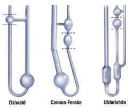
Two general classes of capillary viscometer have found use, namely U-tube viscometers and suspended level viscometers. A common feature of these viscometers is that a measuring bulb, with upper and lower etched marks, is attached directly above the capillary tube. Liquid is either drawn or forced into the measuring bulb form a reservoir bulb attached to the bottom of the capillary tube. The time required for the liquid to flow back between the two etched marks is then recorded.
31 In U-tube viscometer (Ostwald and Cannon-Fenske in Figure 1.11), the pressure head giving rise to flow depends upon the volume of liquid contained in the viscometer. Therefore, it is important to ensure that this volume is the same for each measurement. This is normally achieved after temperature equilibration by adjusting the liquid level to an etched mark just above the reservoir bulb. A further complication in the U-tube viscometers is the need of perfect vertical alignment of the viscometer, since slight deviations from the vertical can give rise to significant changes in the pressure head. This problem is essentially eliminated in the Cannon-Fenske viscometer having the measuring bulb position vertically above the reservoir bulb.
Most suspended level viscometers are based upon the design due to Ubbelohde (Figure 1.11), the most significant feature of which is the additional tube attached just below the capillary tube. This ensures that during measurement the liquid is suspended in the measuring bulb and capillary with atmospheric pressure acting both above and below the flowing column of liquid. These viscometers have a number of advantages in comparison to U-tube viscometers: the variation of pressure head during measurement is smaller, vertical alignment is less critical, and the volume of liquid in the viscometer need not to be constant because the position of the suspended liquid level at the bottom of the capillary is fixed. The latter feature is particularly useful since it enables solutions to be diluted directly in the viscometer. Thus, a known volume of the most concentrated solution is placed into the viscometer and its flow time determined. A known volume of solvent is then added, and through mixing and temperature equilibration, the flow time of the diluted solution is measured. This procedure is then repeated for several dilutions.32
1.5.2.b Types of viscosity
Using a single solution with a pre-determined concentration and a single measurement is possible, with a capillary viscometer, to determine the following kinds of viscosity:
32
Dynamic viscosity
The dynamic (shear) viscosity of a fluid expresses its resistance to shearing flows, where adjacent layers move parallel to each other with different speeds. It can be defined through the idealized situation where a layer of fluid is trapped between two horizontal plates, one fixed and one moving horizontally at constant speed. This fluid has to be homogeneous in the layer and at different shear stresses. The plates are assumed to be very large, so that one need not consider what happens near their edges.
If the speed of the top plate is low enough, the fluid particles will move parallel to it, and their speed will vary linearly from zero at the bottom to u at the top. Each layer of fluid will move faster than the one just below it, and friction between them will give rise to a force resisting their relative motion. In particular, the fluid will apply on the top plate a force in the direction opposite to its motion, and an equal but opposite one to the bottom plate. An external force is therefore required in order to keep the top plate moving at constant speed.33
The magnitude F of this force is found to be proportional to the speed u and the area A of each plate, and inversely proportional to their separation y:
𝐹 = 𝜇𝐴𝑢 𝑦
The proportionality factor 𝜇 in the formula is the dynamic viscosity.
Kinematic viscosity
The kinematic viscosity (also called "momentum diffusivity") is the ratio of the dynamic viscosity μ to the density of the fluid ρ. It is usually denoted by the Greek letter nu ().
𝜈 =𝜇 𝜌
By using a viscometer, it is possible to determine the kinematic viscosity multiplying the flowing time (between the etched marks) of the solution through the capillary by the capillary constant.
33
Reduced viscosity
Reduced viscosity (ηred) is equal to the ratio of the relative viscosity increment ηi to the mass concentration of the polymer (usually g/ml is used as unit):
η𝑟𝑒𝑑 =η𝑖 𝑐 And the increment ηi is:
η𝑖 =
η − η𝑠 η𝑠
Where η𝑠 is the viscosity of the pure solvent and η is the viscosity of the solution.
Inherent viscosity
Inherent viscosity is the ratio of the natural logarithm of the relative viscosity (η𝑟 = η/ηs) to the mass concentration of the polymer:
η𝑖𝑛ℎ =ln (η𝑟) 𝑐
1.5.2.c Determination of intrinsic viscosity and molecular weight
Intrinsic viscosity is a measure of a solute’s contribution to the viscosity of a solution.
The most general relationship between intrinsic viscosity and dilute solution viscosity takes the form of a power series in concentration:
η𝑟𝑒𝑑 = [η] + 𝑘1[η]2𝑐 + 𝑘2[η]3𝑐2+ 𝑘3[η]4𝑐3 + . ..
34
Given this definition, a large number of equations have been recommended for the evaluation of [η] by extrapolation of experimental data. The most commonly encountered are the Huggins equation and the Kraemer equation:
Huggins: η𝑟𝑒𝑑 = [η] + 𝑘𝐻[η]2
Kraemer: η𝑖𝑛ℎ = [η] + 𝑘𝐾[η]2
The Huggins equation is simply a truncation of the series expansion given above. The Kraemer equation is an approximation of the Huggins equation, from which it may be derived assuming that η𝑖 (which appears in the η𝑟𝑒𝑑) is <<1.
So, as it is possible to see from the equations, the intrinsic viscosity is nothing more than the value of reduced viscosity or inherent viscosity extrapolated to the value of null concentration, so:
[η] = lim𝐶→0 η𝑟𝑒𝑑 Or, as well:
[η] = lim𝐶→0 η𝑖𝑛ℎ
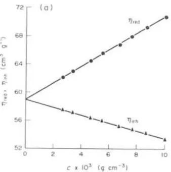
It is now obvious that the easiest way to determine intrinsic viscosity with extrapolation of experimental data is to plot the values of reduced viscosity and/or inherent viscosity and extrapolate those values to the concentration 0. The plot that is obtained is the following.
35
Figure 1.12 – Plot representing variation of inherent and reduced viscosity vs concentration, the interception with the y axis is the intrinsic viscosity32
It is important to observe that the Kraemer representation has always a lower slope than the Huggins one, so the extrapolated intrinsic viscosity is supposed to bring a lower error.
Now that intrinsic viscosity is obtained, it is necessary to evaluate the coefficients K and α to be used in the Mark-Houwink equation.
In order to do that, samples of the polymer of interest with known molecular weight must be used. In fact, given the molecular weight of two or more samples (because there are two variables to determine: K and α), and extrapolated the values of intrinsic viscosity in one of the experimental methods described before, it is possible to use the Mark-Houwink equation to determine the values of K and α relative to those samples.
If the molecular weight of the samples are known to be similar or comparable to those that are still to examine, it is possible to use the K and α evaluated in this way to determine the unknown molecular weight of the polymer using the intrinsic viscosities and, again, the Mark-Houwink equation, this time knowing the value of K and α:
36
1.5.2.d Other ways to determine [𝜼]: the Fedors equation
With the Fedors equation, it is possible to determine the intrinsic viscosity of a polymer without measuring the viscosity of samples at different concentration. The Fedors equation is the following:
1 2(𝜂𝑟12− 1) = 1 [𝜂]𝑐− 1 𝑐𝑚[𝜂]
Where 𝜂𝑟 is the relative viscosity of the solution to a given concentration c and cm are concentration factors that must be calculated using, also in this case, samples with known intrinsic viscosity34
In fact, once given the intrinsic and relative viscosity of an already known sample, it is possible to extrapolate cm from the Fedors equation and use it to determine the intrinsic viscosity of other samples.
Of course, even after this extrapolation, it is possible to determine the molecular weight of the polymer using the obtained intrinsic viscosity and the Mark-Houwink equation.
37
2 Aim of the project
As mentioned before, as the acidic conditions for chitin demineralization (pH, time, and temperature) become harsher, the molecular weight of the products thus obtained becomes lower. Indeed, chitin is an acid-sensitive material and can be degraded by several hydrolytic depolymerization. So, with increasing acid concentration, temperature and time of reaction, we expect the molecular weight of the final product (chitosan) to decrease.
Within the comprehensive framework of the project, as described in the Results and Discussion, the concrete aim of this work is the determination of an empirical mathematical model that must relate the molecular weight of the finally obtained chitosan to the conditions under which its precursor, the chitin, gets demineralized. The decarbonation reaction happens in water medium with a not so high concentration of acid. In this condition, the chitin is not soluble, so, what happens in this step is a solid-liquid heterogeneous reaction; therefore, the determination of a kinetic equation of such a process is surely difficult and for this reason, a semi-empirical approach is essential. In addition, it is not possible to study a wide range of decarbonation conditions such as acid concentration, temperature and time in all their possible values and combinations, because it would require a huge amount of time and especially a lot of experiments. What is necessary is a
technique able to relate aimed experimental data to a representative mathematical
38
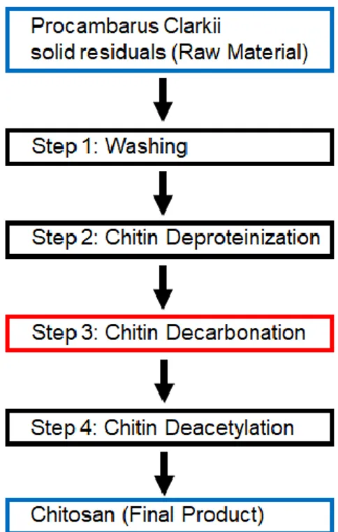
Figure 2.1 – Schematization of the production of chitosan from Procambarus Clarkii solid residuals
The obtained model must allow us to obtain a better understanding of the effects that variations in the decarbonation conditions (Step 3 in figure 2.1) could bring to the molecular weight of chitosan (Final Product). This mathematical model can eventually give us the instructions about the conditions of decarbonation that can lead us to the obtainment of a maximum or a minimum in our response, or rather in the molecular weight of the final product.
So, the obtainment of this model will allow whoever is interested in chitin treatment to operate varying decarbonation conditions knowing what effect these conditions will have on MW of chitosan. This can be considered like an optimization of the process, finalized to the industrial replication and utilization.
39
3 Results and discussion
To achieve the main target of this work, a set of experiments must be planned, in order to minimize the number of intents, although obtaining a representative number of chitosan samples with differences in molecular weight due to the utilization of different decarbonation conditions. Therefore, each of the other three steps reported in figure 2.1 must be carried out with the same conditions for every sample, in order to be sure that variations in chitosan molecular weight are due
only to the decarbonation conditions.
The technique used to plan the experimental work and to analyze the obtained data is the Response Surface Metodology35.
The details about the experimental conditions used for washing, deproteinization and deacetylation are reported in the Experimental Part, while this chapter will focus mainly on the decarbonation step and the analysis of the results with the use of the Response Surface Metodology.
3.1 Response surface methodology
Response Surface Methodology (RSM) is a set of techniques that encompasses35: 1. Setting up a series of experiments (designing a set of experiments) that will
yield adequate and reliable measurements of the response of interest; 2. Determining a mathematical model that best fits the data collected from the
designed chosen, by conducting appropriate tests of hypotheses concerning the model’s parameters;
3. Determining the optimal settings of the experimental factors that produce the maximum (or minimum) value of the response;
If discovering the best value, or values, of the response (the molecular weight MW) is beyond the available resources of the experiment, then Response Surface Methodologies are aimed at obtaining at least a better understanding of the overall process. However, in the cases examined in this work of thesis it possible to discover the maximum and the minimum value of MW obtainable, but the
40
relationship between the factors (acid concentration, temperature and time) and the response is too complex and unknown, so an empirical approach is necessary.
3.1.1 Design of experiment: general notes on the Central Composite Design The design of experiment (DoE) is a statistical tool that directs and minimizes the needed experimentation, to obtain a mathematical model representative of the process with enough precision and robustness. There are many types of DoE, depending on the number of factors (in our case three: concentration, temperature, reaction time) and the resolution of the problem that we desire. In any case, the number of experiments always rises with the number of factors and with the resolution of the problem that we want.
In our case, we will use a Central Composite Design (CCD), which is the most commonly used when there are three or more factors and when there is the need to obtain a complete understanding of the influence of the factors and their synergic interaction on a single response (MW).
The CCD consists of three portions, each of them is constructed using points given by single experiments with certain conditions:
One portion (F) corresponding to a fractional design, with 2k points, where k is the number of factors;
One axial portion, corresponding to experiments along the axes of the factors, at a distance (α) from the center of the design. It will consists of 2k points;
One central portion (nc), containing the central experiment and its repetitions.
Therefore, the minimum number of experiments is given by 𝑁 = 𝐹 + 2𝑘 + 𝑛𝑐
Where nc is the number of central points (1) more the number of its repetitions that must be done in order to evaluate the pure experimental error of the method (in our case we did 3 repetitions), so it becomes:
41 𝑁 = 8 + 2𝑥3 + 4 = 18
The value of α, which is the half length of the axis of each factor is α = 𝐹1/4= 1,682
A graphic representation of our CDD is constructed like this: (Figure 3.1)
Figure 3.1 - Graphic representation of the Central Composite Design (CCD)
The yellow point is the central point, which represents the experiment with the intermediate conditions of acid concentration, temperature and time, and, as said before, must be repeated an adequate number of times in order to evaluate the pure experimental error of the method; the other colored points represent the axial portion, while the black ones represent the fractional portion. Therefore, each of the points represents a single experiment with its own conditions of acid
42
concentration, temperature and time; as it is shown here. There are a total of 15 experiments (and the repetitions of the central point must be added).
To fit in this kind of design and to have each of the factors not dependent from its measure unit, each factor real value must be “codificated” in dimensionless values between -1,682 and +1,682 (– α and α), for example, the maximum concentration of acid will have the +1,682 value, while minimum concentration -1,682, and the same for the other parameters. This allows us to compare the relative importance of each factor.
Anyway, before the codification, it is necessary to determine the real upper and lower limits of acid concentration, temperature and time, in order to obtain the value of – α and α of each factor.
3.1.1.a Preliminary study: Determination of upper and lower limits Acid concentration
To evaluate the lower limit of acid concentration, we have calculated stoichiometrically which was the theoretical acid concentration needed to remove all the calcic carbonate present in the deproteinized matter.
The quantities involved for the decarbonation were 35 grams of matter (with ~70% of calcic carbonate) in 350 ml of acid solution.
𝑔 𝐶𝑎𝐶𝑂3 = 35 𝑔 ∗ 0,70 = 24,50 𝑔 𝐶𝑎𝐶𝑂3 So:
𝑚𝑜𝑙𝑒𝑠 𝐶𝑎𝐶𝑂3 = 24,50 𝑔 𝐶𝑎𝐶𝑂3
100,087 𝑔/𝑚𝑜𝑙= 0,245 𝑚𝑜𝑙𝑒𝑠 𝐶𝑎𝐶𝑂3 The reaction of decarbonation is:
CaCO3 + 2HCl H2O + CO2(g) + CaCl2
So, the minimum number of moles of HCl needed to remove all the calcic carbonate is:
43 Which, divided by 0,350 L, that is the volume of solution used, gives 1,4 mol/L (~1,5 mol/L), which is the minimum acid concentration needed and the one used for this work. It would not make any sense using a solution less concentrated because, since the decarbonation reaction is very fast, almost all the acid would be used to remove the calcic carbonate and the acid hydrolysis of the polymeric chain would barely not happen.
To determine the upper limit of acid concentration, several experiments were carried out. As a wider range of concentration could give us a better understanding of the effect on molecular weight, a high concentration of acid (9 mol/L) was tested. The result was the formation of black particles, permanent even after the deacetylation to chitosan and totally insoluble, and for this reason very inconvenient for any successive MW measurement or treatment. This could be explained by the occurrenceof a reaction similar to the carbonization of a polysaccharide by acid treatment, in this case acting on chitin. A picture of these black particles is shown below (Figure 3.2):
Figure 3.2 – Black particles left after treatment with 9 M HCl
After several intents varying concentration, the acidity settled for the experimental design was 3,5 mol/L of acid, which proved to give (after the successive deacetylation of chitin) soluble chitosan with no black particles.
44
Temperature
The lower limit of temperature was easy to settle as, to avoid the use of a refrigeration cycle which could be expensive also in an industrial context, we simply decided to put the room temperature (measured for each experiment, but always around 25 °C) as lower limit.
The upper limit was decided using the same attempts explained in the determination of the acid concentration limit. In first place, we tried 90° C as upper limit, but we assisted to the formation of the black particles already mentioned. We thought that the carbonization reaction was facilitated by the high temperature, so we lowered the temperature, and the result was the disappearance of the black particles.The actual upper limit was finally settled to 65 °C.
Time
The lower time limit was settled consulting a previous work done from the research group36. In this work, it is explained and proven that the minimum time to remove all the calcic carbonate using acid concentrations very similar to the lowest one (1,8 mol/L vs the 1,5 mol/L we used), is 23,43 minutes measured at room temperature. Therefore, taking account that only a few experiments would have been done at room temperature and all the others at higher temperatures, we settled 30 minutes as lower limit, supposing that after 30 minutes all the calcic carbonate would have been dissolved.
The upper time limit was settled consulting the same work, where, after 180 minutes at room temperature, all the calcic carbonate was removed. As said before, only a few reaction were expected to be done at room temperature, and in order to minimize the needed time, we decided to set 150 minutes as upper time limit.
The limits of the design in the axial portion settled in the ways described are summarized in the table below:
45 -α +α Conc. HCl (mol/L) 1,5 3,5 Temperature (°C) 25 65 Time (min) 30 150 2.1.1.b Design of Experiment
After having settled the upper and lower limit of each variable, we proceeded with the actual construction of the whole experimental design.
A three-factor Central Composite Design is always built like shown in the Table 3.1 below. The points in Figure 3.2 are nothing else than a graphic representation of the trials reported in the table:
Trial [HCl] Temper. Time
•
1 -1 -1 -1•
2 1 -1 -1•
3 -1 1 -1•
4 1 1 -1•
5 -1 -1 1•
6 1 -1 1•
7 -1 1 1•
8 1 1 1•
9 0 0 0•
9 0 0 0•
9 0 0 0•
9 0 0 0•
10 α 0 0•
11 - α 0 0•
12 0 α 0•
13 0 - α 0•
14 0 0 α•
15 0 0 - αTable 3.1 – Complete set of experiment with codificated values provided by this experimental design
46
We had to make a correspondence between the values in the table, that are dimensionless and codificated for the design and the real values of the factors. The values of +α and –α (+ 1,682 and -1,682) for every factor are respectively their upper and lower limit. While the values of -1, 0 and 1 are calculated simply using a proportion, for example: the value of the “0” of concentration is nothing else than the intermediate value of concentration between the upper and lower limit, or rather 2,5 mol/L.
The correspondence between the real values and the codificated ones is reported in the table below:
-α -1 0 1 +α
Conc. HCl (mol/L) 1,5 1,9 2,5 2,9 3,5
Temperature (°C) 25 33 45 54 65
Time (min) 30 54 90 126 150
Table 3.2 – Correspondece between codificated values and real values of the factors
2.1.2 Determination of the mathematical model
The determination of the mathematical model relating molecular weight of chitosan with the conditions of decarbonation was achieved using a statistical software named “ECHIP7” (Figure 3.4).
47 Inserting the codificated design variables of each experiment (like for example – α;0;0, 0;0;0 ecc..) and their respective value of the response (molecular weight, viscosity or any other one), it is possible, through the software, to obtain a statistical analysis of the experiments, including the mathematical model seeked for this work. It is also possible to see 3D graphs showing the trend of the response under the simultaneous variation of two of any of the three factors.
The determination of the mathematical model comes through the method of least squares.
Method of least squares
The method of least squares is a mathematical procedure for finding the best-fitting curve to a given set of points by minimizing the sum of the squares of the offsets (the residuals i.e the difference between an observed value, and the fitted value provided by a model) of the points from the curve(Figure 3.4).
Figure 3.4 – Graphic representation of the residuals in a typical plot Response Variable vs Design Variable
The procedure, carried out by the software, is an algebric procedure for fitting linear equations to data:
48
Figure 3.5 – Graphic example of a regression analysis
As an example, in the picture above (Figure 3.5), the blue curve is the result of a regression analysis done with the method of least squares on a set of experimental points (red).
Optimization
After having established the model that best fits the experimental data, the software can proceed with the optimization.
It is possible to see which are the optimal conditions to obtain a maximum or a minimum of the response. Obviously, as the graph shown are 3-axis graphs, one of the three factors must be fixed to a value, while the other two change their value in order to find the seeked optimal of the response.
49
Figure 3.6 – Example of a 3D graph provided by the software ECHIP7
3.2 Analysis of the results
3.2.1 Collection of the data
The first part of the work was the application of the experimental design planned in Table 3.1. It is important to say that the order with whom the experiment had to be done is not the order of the experiment showed in the Table 3.1, indeed the order of the experiments must be random, to remove from the results every possible pattern due to the order of execution.
After the decarbonation done with the conditions described from the design, each sample had to be deacetyated to chitosan to make it soluble (chitin is not soluble in conventional solvents) and its MW measurable.
Therefore, each sample derived from the decarbonation was deacetylated under the same conditions:
NaOH 50% w/w Temperature 120 °C Reaction time 120 minutes
50
We chose to apply the same conditions for the deacetylation to be sure that the only factors affecting the differences between the molecular weight of the chitosan samples were derived from the different decarbonation conditions.
At this point we had 18 chitosan samples and we had to measure their molecular weight.
To measure the molecular weight of the chitosan samples we chose to use the viscosimetry method, as it is the one of the simplest and cheapest way to measure molecular weight of a polymer.
The instructions on how to apply viscosimetry for chitosan MW calculation were found in bibliography37.
We used a Cannon-Fenske viscometer (Figure 3.7), with a viscometer constant of 0,041796 cSt/s.
The solvent used to solubilize the polymer was a 0,25 M/0,25 M tampon solution of HAc/NaAc.
We decided to collect the flowing times at different concentration in all the works found in bibliography about the determination of molecular weight of chitosan37, viscosities at different concentrations were required. Moreover, having data at different concentrations allows a more accurate data extrapolation and analysis regarding the viscosity properties of the polymer.
Therefore, for each sample, the flowing time of a solution containing 0,00576 g/ml of chitosan was measured. Then, each sample was diluted 20% using the tampon solution, and its flowing time was measured again; this process was repeated until we had five flowing times for each sample, one for the mother solution and four for its successive 20% dilution:
0,00576 g/ml 0,00461 g/ml 0,00369 g/ml 0,00295 g /ml 0,00236 g /ml
Figure 3.7 – Cannon-Fenske
51 3.2.2 Analysis of the first response: Kinematic Viscosity
After the collection of the flowing times of each of the samples planned from the experimental design, we needed some data elaboration to reach the seeked mathematical model.
The first and most standing out result obtained from the viscosimetry is the kinematic viscosity of the mother solution, in fact, as it was explained in the introduction, simply multiplying the flowing time of a solution by the constant of the capillary viscometer the kinematic viscosity of the solution is obtained.
Even if with the kinematic viscosity we could not have an actual relation of the decarbonation conditions with the molecular weight, we were sure that the variation of the kinematic viscosity was directly related with the variation of molecular weight, as a decrement of molecular weight of a polymer surely brings a decrement in the viscosity of that polymer solution.
Therefore, we multiplied the flowing times of each sample by the constant of the viscometer, and what we obtained is shown in the table below:
Trial [HCl] Temper. Time Kinematic Viscosity (cSt) 1 -1 -1 -1 12,08 2 1 -1 -1 8,45 3 -1 1 -1 5,77 4 1 1 -1 3,65 5 -1 -1 1 7,58 6 1 -1 1 3,53 7 -1 1 1 3,13 8 1 1 1 3,01 9a 0 0 0 3,79 9b 0 0 0 4,18 9c 0 0 0 3,96 9d 0 0 0 4,00 10 α 0 0 3,05 11 - α 0 0 6,34 12 0 α 0 2,24 13 0 - α 0 5,47 14 0 0 α 4,02 15 0 0 - α 8,43