Alma Mater Studiorum – Università di Bologna
Scuola di Scienze
Dipartimento di Fisica e Astronomia
Corso di Laurea magistrale in Astrofisica e Cosmologia
A wide frequency study of the spectral
properties of cores and lobes of radio galaxies
Tesi di laurea
Presentata da:
Relatore:
Daniele d'Antonio
Chiar.mo Prof.
Gabriele Giovannini
Correlatore:
Dott. Marcello Giroletti
Sessione II
to my parents
and
my sister
Sommario
Le osservazioni alle basse frequenze stanno aprendo nuovi scenari per lo studio del cielo, per caratterizzare sia nuovi fenomeni che le gi`a note classi di sorgenti. In questo lavoro vengono caratterizzate le propriet`a spettrali della popolazione dei blazar osservati a basse frequenze, vengono comparate le propriet`a in banda radio e ad alte energie dei gamma-ray blazars, e ven-gono cercate le controparti radio delle sorgenti gamma non identificate.
In un precedente lavoro (Giroletti et al. 2016), i 6100 gradi quadrati del Murchison Widefield Array Commissioning Survey catalogue (MWACS) sono stati cross-correlati con il terzo catalogo di nuclei galattici osservati da F ermi. Con il lavoro svolto in questa tesi, i 24831 gradi quadrati del Galactic and Extragalactic All-sky MWA (GLEAM) con lo stesso catalogo di F ermi. Paragonato ad MWACS, GLEAM non ha solo pi`u grande area di cielo, ma anche una migliore sensibilit`a e una maggiore copertura spettrale. La frazione di gamma-ray blazars riportati in GLEAM cresce sino a raggiun-gere il 78%, rispetto al 45% ottenuto con MWACS.
In particulare, sono stati considerati blazar classificati in base alla fre-quenza del picco di sincrotrone e alle righe di emissione: `e stato esaminato il comportamento di oggetti high-, intermediate- e low-synchrotron peaked (HSP, ISP, LSP, rispettivamente) e di flat spectrum radio quasars(FSRQs), BL Lacertae(BLL) e di blazars di tipo non identificato (BCU). L’aumento di detection rate per gli oggetti con picco di sincrotrone a pi`u alta frequenza
di oggetti, dal punti di vista della statistica: gli LSP e gli FSRQ sono gli le sorgenti pi`u numerose ad alti redshift, in particolar modo a z 2, mentre gli HSP aumentano a bassi redshift; anche le emissioni in banda X e radio presentano diversi dati statistici: gli HSP presentano una maggiore emissione nell’X rispetto agli LSP e agli FSRQ, ma quest’ultimi presentano maggiore emissione nel radio (sia a basse, a intermedie che ad alta frequenze). Gen-eralmente i BL Lac sono pi`u eterogenei, e presentano molta dispersione nei vari plots. D’altra parte, gli LSP e gli FSRQ coincidono con la stessa sor-gente in molti casi. Infatti `e stata eseguita una cross-correlazione delle due popolazioni e sono stati osservati molti matches (238 per un totali di 267 FSRQ). Grazie alla grande copertura spettrale a disposizione di GLEAM e di altre survey radio, sono state studiate le propriet`a dei blazar a bassa ( 200MHz), intermedia ( 1GHz), e alta frequenza (20GHz con l’Australia Telescope 20GHz, AT20G). Nuclei compatti e lobi estesi hanno differenti propriet`a spettrali: a bassa frequenza `e stata esaminata l’emissione estesa, mentre ad alta frequenza `e stato esaminato il nucleo. Quindi, determinando lo spettro delle sorgenti in diverse bande di frequenza `e stato possibile stimare il rapporto tra le due componenti di emissione (componente estesa e compo-nente del nucleo), ed `e stata ottenuta una stima della core dominance. La core dominance di un oggetto corrisponde ad un test che verifica l’esattezza del Modello Unificato degli AGN. Gli oggetti con un indice spettrale pi`u piatto sono pi`u core dominated, mentre gli oggetti con indice spettrale pi`u ripido sono pi`u lobe dominated. In generale, il grande campo di vista delle survey a basse frequenze e il grande sviluppo tecnologico in questo campo, in preparazione dello Square Kilometre Array stanno portando una vera e propria rivoluzione.
Infine `e stata costruita una simulazione di una survey di oggetti, mediante il linguaggio di programmazione Python, con l’obiettivo di confrotare i dati
iii
misurati con dei dati virtuali e verificare la correttezza del nostro metodo di ricerca. Inoltre per stimare l’emissione del nucleo delle sorgenti a dispo-sizione, `e stata utilizzata la survey FIRST Faint Images of the Radio Sky at Twenty, una survey con ottima risoluzione angolare (5 arcsec). L’obiettivo della simulazione `e stato quello di verificare quanto questa risoluzione sia ef-fettivamente adatta per studiare l’emissione del nucleo di una radio sorgente.
Contents
1 Active Galaxies: theorical background 1 1.1 Active Galactic Nuclei (AGN) . . . 1 1.1.1 AGN classification . . . 3 1.1.2 The Spectral Energy Distribution (SED) of blazars . . 4 2 Observing instruments 7 2.1 A precursor for SKA: the Murchison Widefield Array (MWA) 7
2.1.1 The Murchison Widefield Array Commisioning Survey (MWACS) . . . 8 2.1.2 The GaLactic and Extragalactic All-sky MWA (GLEAM) 9 2.2 The Very Large Array (VLA) . . . 11 2.2.1 The NRAO VLA SKY SURVEY (NVSS) . . . 11 2.2.2 The Faint Images of the Radio Sky at Twenty (FIRST) 12 2.3 The Australia Telescope Compact Array (ATCA) . . . 13 2.3.1 The Australia Telescope 20-GHz Survey (AT20G) . . . 13 2.4 The Roma BZCat . . . 14 2.5 The Sloan Digital Sky Survey (SDSS) . . . 15 2.6 The F ermi satellite . . . 15 2.6.1 The third catalogue of the Fermi-LAT (3FGL) . . . . 16 3 Cross-correlations of catalogues 23 3.1 Cross-correlation for the GLEAM and the 3LAC . . . 24 3.2 Cross-correlation for the AT20G and the 3LAC . . . 25 3.3 Cross-correlation for the AT20G and the GLEAM . . . 26
3.4 Cross-correlation for the 3LAC and AT20G-GLEAM . . . 27
3.5 Cross-correlation for the BZCat and GLEAM . . . 28
3.6 Cross-correlation 3LAC-GLEAM and BZCat-GLEAM . . . . 28
3.7 Anticross-correlation BZCat-GLEAM and 3LAC-GLEAM . . . 29
3.8 Cross-correlation for SDSS-FIRST-NVSS and GLEAM . . . . 30
3.9 Cross-correlation 3LAC-GLEAM and 3LAC-AT20G . . . 31
3.10 Statistics . . . 31
4 Results about the spectral properties for blazars detected at low frequency 35 4.1 Detection rate: a jump from MWACS to GLEAM . . . 35
4.1.1 Multi-wavelength and spectral statistical properties . . 36
4.2 Multi-wavelength properties . . . 41
4.3 Discussion about the FSRQs and LSP . . . 50
4.4 Discussion about the BL Lacs and HSP . . . 51
4.5 Summary of the spectral properties . . . 52
4.6 A further study of the spectral properties of gamma-ray blazars 53 5 Results about the radio cores and the lobes for radio loud AGN 55 5.1 Correlation between gamma-rays and high frequency radio emission . . . 55
5.2 A test for the Unified Model of AGN: the core dominance . . 56
5.3 Lobes component and core component in a spectrum of radio loud AGN . . . 64
Conclusions 71
A Code simulation of radio sources 75
List of Figures
1.1 a scheme for the AGN Unified Model from Beckmann Shrader et al. 2012. In the top part of the graphic there are the loud sources, in the bottom part there are the radio-quiet sources. . . 2 1.2 Spectral Energy Distribution for a blazar, with the synchrotron
peak (left) and the inverse Compton peak (right). In the most luminous sources the synchrotron peak and the IC peak are at lower frequency (Donato et al. 2001). . . 6 2.1 MWA is located in the australian desert, in the Western
Aus-tralia . . . 8 2.2 Survey of the MWACS with galactic coordinates (Hurley-Walker,
et al. 2014). The dark regions are the areas with largest source density. . . 9 2.3 Survey of the GLEAM with galactic coordinates (Hurley-Walker,
et al. 2017). The dark regions are the areas with largest source density. . . 10 2.4 The Very Large Array is located in New Mexico, USA. . . 11 2.5 The Australia Telescope Compact Array (ATCA) is located
at ∼ 500 km north-west of Sydney, (Australia). . . 13 2.6 rappresentation of the F ermi satellite. . . 16 2.7 Survey of the 3LAC with galactic coordinates (Ackermann, et
al. 2015). . . 18 vii
2.8 redshift distributions (solid: 2LAC sources; dashed: new 3LAC sources) for FSRQs (top), BL Lacs (middle), and different types of BL Lacs (bottom): LSPs (green), ISPs (light blue), and HSPs (dark blue). The ranges between the lower and up-per limits are also depicted in the bottom panel when both limits are available (Ackermann et al. 2015). . . 19 2.9 Photon spectral index distributions. Top: FSRQs (solid: 2LAC
sources; dashed: new 3LAC sources). Second from top: BL Lacs (solid: 2LAC sources; dashed: new 3LAC sources). Third from top: 3LAC LSP-BL Lacs (green), ISP-BL Lacs (light blue), and HSP-BL Lacs (dark blue). Bottom: blazars of un-known type (solid: 2LAC sources; dashed: new 3LAC sources) (Ackermann et al. 2015). . . 20 2.10 Photon spectral index vs. photon flux above 100 MeV for
blazars in the 3LAC Sample. Red circles: FSRQs; blue circles: BL Lacs; green triangles: blazars of unknown type; magenta stars: other AGNs. The solid (dashed) curve represents the approximate 3FGL (2FGL) detection limit based on a typical exposure. The 2FGL is the second catalog of F ermi while the 3FGL is the third catalog (Ackermann et al. 2015). . . 21 3.1 Survey of the blazars with a counterpart at low-frequency
(3LAC vs. GLEAM). Obviously the sources are in the sky area of the GLEAM survey. . . 25 3.2 Survey of the detected blazars at high frequency (3LAC vs.
AT20G). The most objects are in the Southern sky. Infact the most sources of the AT20G are in the same sky. . . 26 3.3 Survey for radio sources at low and high frequency (AT20G
vs. GLEAM). . . 27 3.4 Survey for blazars selected at low and high frequency (3LAC
INDEX ix
3.5 Survey radio sources at low and intermediate frequency (BZ-Cat vs. GLEAM). . . 28 3.6 Survey for the blazars selected at low and intermediate
fre-quency (3LAC-GLEAM vs. BZCat-GLEAM). . . 29 3.7 Survey for the anticross-correlation BZCat-GLEAM and
3LAC-GLEAM. . . 30 3.8 Survey of radio sources selected at low and intermediate
fre-quency (SDSS, FIRST, NVSS, GLEAM). . . 30 3.9 Survey of blazars detected at low and high frequency
(3LAC-GLEAM vs. 3LAC-AT20G). . . 31
4.1 radio flux density at 1GHz distribution for the entire 3LAC sample (red) in the GLEAM sky and 3LAC sources with a GLEAM counterpart (blue). . . 37 4.2 gamma-ray flux at E > 100 MeV distribution for the entire
3LAC sample (red) in the GLEAM sky and 3LAC sources with a GLEAM counterpart (blue). . . 37 4.3 normalized flux density distribution at low frequency for all
GLEAM sources (green) and low frequency detected blazars (blue). Blazars are brighter then the rest of GLEAM sources. 40 4.4 normalized spectral index distribution for the blazars detected
at low frequency (blue) and all GLEAM sources (green). The blazars are flatter-spectrum objects than the rest of the sam-ple. . . 40 4.5 correlation between radio emission at low frequency and radio
emission at intermediate frequency. Spectroscopic classifica-tion (left): FSRQs (red), BLL (blue), BCU (green). SED clas-sification (right): LSP (magenta), ISP (green), HSP (cyan). The solid lines show best fit regression. . . 42
4.6 correlation between gamma emission and radio emission at in-termediate frequency. Spectroscopic classification (left): FSRQ (red), BL Lac (blue), BCU (green). SED classification (right): LSP (magenta), ISP (green), HSP (cyan). . . 43 4.7 correlation between gamma emission and radio emission at
low frequency. Spectroscopic classification (left): FSRQ (red), BL Lac (blue), BCU (green). SED classification (right): LSP (magenta), ISP (green), HSP (cyan). . . 43 4.8 redshift distribution. Spectroscopic classification (left):
FS-RQs (red), BCUs (green), BL Lacs (blue). SED classification (right): LSP (magenta), ISP (green), HSP (cyan). . . 45 4.9 Plot of X-ray flux vs. radio density flux. Spectroscopic
clas-sification (left): FSRQs (red), BL Lacs (blue), BCUs (green). SED classification (right): LSP (magenta), ISP (green), HSP (cyan). . . 45 4.10 Plot of gamma-ray flux vs. X-ray flux. Spectroscopic
clas-sification (left): FSRQs (red), BL Lacs (blue), BCU (green). SED classification (right): LSP (magenta), ISP (green), HSP (cyan). . . 48 4.11 photon index vs. synchrotron peak. Spectroscopic
classifi-cation (left): FSRQs (red), BL Lacs (blue), BCUs (green). SED classification (right): LSP (magenta), ISP (green), HSP (cyan). . . 48 4.12 photon index vs. gamma luminosity. Spectroscopic
classifi-cation (left): FSRQs (red), BL Lacs (blue), BCUs (green). SED classification (right): LSP (magenta), ISP (green), HSP (cyan). . . 49 4.13 gamma luminosity vs. redshift. Spectroscopic classification
(left): FSRQs (red), BL Lacs (blue), BCUs (green). SED clas-sification (right): LSP (magenta), ISP (green), HSP (cyan). . 49
INDEX xi
5.1 gamma emission vs. radio emission at high frequency. Spec-troscopic classification (left): FSRQs (red), BL Lacs (blue), BCUs (green). SED classification (right): LSP (magenta), ISP (green), HSP (cyan). . . 56 5.2 GLEAM spectral index vs. ratio between flux density at 20
GHz (core emission) and flux density at 200 MHz (extended emission). . . 58 5.3 core power vs. total power for the sample AT20G-GLEAM
(red) and the sample of Giovannini et al. 1988 (blue). . . 59 5.4 spectral index vs. ratio between flux density of FIRST (core
emission) and flux density of NVSS (extended emission). . . . 60 5.5 core power vs. total power for the sample SDSS-FIRST-NVSS
(green) and the sample of Giovannini et al. 1988 (blue). . . . 62 5.6 core power vs. total power for the sample SDSS-FIRST-NVSS
(green) and the sample of Giovannini et al. 1988 (blue). We considered the deamplification of the core emission due to red-shift. . . 63 5.7 three examples for a spectrum of an AGN: the sum of the steep
component (red) and the flat component (blue), produces the total spectrum (green). From the first spectrum (left) to the third spectrum (right) ratio between lobe and core emission decreases, and the overall spectrum flattens. In our case, the green line is the GLEAM spectrum, composed of two contri-butions, and we use it to constrain the relative weight of the extended (red) and nuclear (blue) components. . . 66 5.8 distribution of the ratio Klobe/Kcore. . . 69
A.1 redshift distribution: the number of sources increases with the redshift. The red curve describes the distribution for the objects detected. . . 77 A.2 distribution of intrinsic size of the sources. The red curve
A.3 viewing angle distribution: increasing the angle the number of sources undetected increases. Instead the sources detected do not increase then about 5 degree. The red curve describes the distribution for the objects detected. . . 80 A.4 spectral index distribution: we assumed a Gaussian
distribu-tion for all objects. The red curve describes the distribudistribu-tion for the objects detected. . . 82 A.5 luminosity distance distribution: increasing the luminosity
distance the number of sources increases. The red curve de-scribes the distribution for the objects detected. . . 84 A.6 angular diameter distance distribution: increasing the angular
diameter distance the number of sources increases. The red curve describes the distribution for the objects detected. . . . 84 A.7 projected angular size distribution: the number of sources
de-creases with the size. The red curve describes the distribution for the objects detected. . . 85 A.8 projected angular size distribution with three ranges: <4.5”(red),
4.5”-45”(magenta), >45”(black). . . 87 A.9 Doppler factor distribution: we see a similar behaviour for
observed and unoberserved objects. The red curve describes the distribution for the objects detected. . . 88 A.10 luminosity distribution: the number of the sources undetected
decreases with the luminosity, while for the sources detected is true the opposite. The red curve describes the distribution for the objects detected. . . 89 A.11 flux density distribution: we observe only the sources over 1
mJy. The red curve describes the distribution for the objects detected. . . 91
List of Tables
2.1 angular resolution for the MWA. . . 8
2.2 technical features for the MWACS . . . 9
2.3 technical features for the GLEAM . . . 10
2.4 technical features for the NVSS . . . 12
2.5 technical features for the FIRST . . . 12
2.6 technical features for the AT20G . . . 14
2.7 technical features for the BZCat . . . 14
2.8 technical features for the SDSS . . . 15
2.9 technical features for the 3FGL. We can see that the source density is very low compared to the source density in the radio surveys . . . 17
2.10 angular resolution for the 3FGL. The resolution rises to the drop in energy. Infact the resolution varying with energy ap-proximately as E−0.8. . . 17
3.1 statistical data for the cross-match 3LAC vs. AT20G. . . 32
3.2 statistical data for the cross-match AT20G vs. GLEAM. We have not data for SED and spectroscopic classifications. . . 33
3.3 Statistical data for the cross-match 3LAC vs. AT20G-GLEAM 33 3.4 statistical data for the cross-match BZCat vs. GLEAM. We have not data for SED and spectroscopic classifications. . . 33
3.5 statistical data for the cross-match 3LAC-GLEAM vs. BZCat-GLEAM . . . 34
3.6 statistical data for the cross-match SDSS-FIRST-NVSS vs. GLEAM. We have not data for SED and spectroscopic classi-fications. . . 34 3.7 statistical data for the cross-match GLEAM vs.
3LAC-AT20G. We have not data for SED and spectroscopic classifi-cations. . . 34 4.1 The detection rate from MWACS to GLEAM grows for every
kind of object. . . 38 4.2 values for the logarithm of the radio (∼ 1GHz) flux density
Frad, X-ray flux FX and gamma-ray flux Fγ. The associated
errors are the standard deviations. . . 39 4.3 mean values for the spectral index with the total number of
blazars detected at low frequency and the number of sources with a value of the spectral index α. The associated errors are the standard deviation. . . 41 4.4 values for the correlation coefficient r for the correlation
be-tween radio emission at intermediate frequency and radio emis-sion at low frequency. . . 44 4.5 values for the correlation coefficient r for the correlation
be-tween gamma emission and radio emission at intermediate fre-quency. . . 46 4.6 values for the correlation coefficient r for the correlation
be-tween gamma emission and radio emission at low frequency. . 47 4.7 values for the correlation coefficient r for the plot X emission
vs. radio emission at intermediate frequency. . . 50 4.8 values for the correlation coefficient r for the plot gamma
emis-sion vs. X emisemis-sion. . . 51 4.9 results for gamma-ray blazars (data of the cross-correlation
INDEX xv
4.10 results for blazars without an important emission in the gamma band (data of the anticross-correlation BZCat-GLEAM vs. 3LAC-GLEAM). . . 54
5.1 values for the correlation coefficient r for the plot gamma emis-sion vs. radio emisemis-sion at high frequency. . . 57 5.2 value for the correlation coefficient r for the correlation
spec-tral index vs. ratio between flux density at 20 GHz (core emission) and flux density at 200 MHz (extended emission). . 57 5.3 values for the correlation coefficient r and the angular
coef-ficient m for the samples AT20G-GLEAM and Giovannini et al. 1988 for the plot core power vs. total power. . . 59 5.4 value for the correlation coefficient r for the plot spectral index
vs. ratio between flux density of FIRST (core emission) and flux density of NVSS (extended emission). . . 61 5.5 results about the mean spectral index and the flux density
ra-tio. In the third column there is the error (standard deviation) for the mean spectral index. . . 61 5.6 values for the correlation coefficient r and the angular
coef-ficient m for the samples SDSS-FIRST-NVSS-GLEAM and Giovannini et al. 1988 for the plot core power vs. total power. 62 5.7 values for the correlation coefficient r and the angular
coef-ficient m for the samples SDSS-FIRST-NVSS-GLEAM and Giovannini et al. 1988 for the plot core power vs. total power. We considered the deamplification of the core emission due to redshift. . . 64
A.1 ranges of angular resolution: we see different visibility of the FIRST and the NVSS. . . 86 A.2 legend for the physical parameters. . . 92
A.3 physical parameters (see the Table A.2) with the associated errors. We indicate with meam value1 and SD1 the mean value and the associated error of the simulation, mean value2 and SD2 are the measures of the true catalog SDSS-FIRST-NVSS. Instead mean value3 and SD3 are the measures of the the cross-correlation SDSS-FIRST-NVSS vs. GLEAM. For the luminosity and the flux density we have two values of the true samples. In the upper line we have the values of the FIRST, while in the bottom line we have the values of the NVSS. . . 93 A.4 mean angular size and number of beams included in a radio
Introduction
This work is a study of the radio spectral properties of the most extreme objects in the class of AGN (Active Galactic Nuclei): the blazars. These sources present relativistic plasma jets closely aligned with the line of sight, and for this reason, these objects are detected at high cosmological distances. Infact the emission is amplified by the Doppler boosting. Their emission is mainly non-thermal with a two-humped spectral energy distribution. The blazars are poorly studied at low frequency, being flat-spectrum sources. However, in this work we show a study of their spectral properties, using the deepest, largest and with best sensitivity survey: the GaLactic and Extra-galactic All-sky MWA Survey (GLEAM). Infact it is the first time that it is possible to execute a so accurate study of the blazars at low radio frequency. Moreover, in the last years the astrophysics of the gamma-rays has greatly developed, thanks the advent of the Large Area Telescope (LAT) on board of the F ermi satellite. So we studied the possible correlation between radio and gamma-ray emission. This relation is an important issue to understand the emission process for the blazars.
Moreover, we studied the relation between the core emission and the ex-tended emission in AGN. In particular, we examined the behaviour of the core and extended emission with the spectral index, to verify the presence of a flatter spectrum for core dominated objects and of steeper spectrum lobe dominated objects. In other words, we executed a test for the Unified Model of AGN.
Anyway, the thesis is laid out as follows: there are two introductive chap-ters: the first chapter is a theorical background for AGN (especially blazars), while the second chapter explains the technical features of the strumentation used to create the survey catalogs used in this work. In particular the second chapter shows the characteristics of the Murchison Widefield Array (MWA), a precursor of the Square Kilometre Array (SKA). This is a new genera-tion revolugenera-tionary aperture synthesis radio telescope, with a large field of view and a great sensitivity (of the order of the µJy), and that will be an ideal instrument to characterize the properties of every kind of radio sources. The third chapter shows the differents cross-correlations between the cata-logs used in this work. The cross-correlation allows us to find a counterpart of every source in another frequency range, so it is possible to examine an object in different frequency bands, in different emission regions. The fourth chapter shows the study of the spectral properties for blazars, instead the fifth chapter is the study of the properties of the extended and core emission for AGN.
The work yet explained is the main part of the thesis, but there is a second part in the Appendix, where we show a creation of a simulation of radio sources. The simulation is useful to understand the importance of the core in a radio source, and in general to understand the properties of a survey of radio sources. So we can compare the simulation data with the true data and to obtain some results.
Chapter 1
Active Galaxies: theorical
background
1.1
Active Galactic Nuclei (AGN)
Some galaxies in our universe show a significant excess emission respect that ascribed to stellar processes. These objects are about 1% of the observed galaxies, and they have a typical luminosity about 1042-1048erg/s. This huge
power cannot be only attributed to dust, gas and stars but there is another type of source. It is in the centre of these galaxies, called Active Galactic Nucleus (AGN), while the host galaxy is called active galaxy. The central engine for these galaxies is a supermassive black hole (SMBH) with a mass of 106−109M
, so the surrounding matter must fall towards the centre, causing
dissipation of the angular momentum with the formation of an accretion disk. The causes of the dissipation are the viscosity and the turbulent motion of the gas. However, the basic structure is composed by an accretion disk, a Broad Line Region (BLR), a Narrow Line Region (NLR), a thick torus and two jets. We explained that the gas of accretion disk presents dissipation, viscosity and turbulent motion. With these phenomena the adjacent regions of the disk heat each other, so we have thermal emission of a black body. Clearly the disk is affected by the presence of the black hole, in fact it is
Figure 1.1: a scheme for the AGN Unified Model from Beckmann Shrader et al. 2012. In the top part of the graphic there are the radio-loud sources, in the bottom part there are the radio-quiet sources.
relativity close (about 10−3 pc). Instead the BLR is about 0.01-0.1 pc from the SMBH, and it is composed by gas with a velocity of about 500-104 Km/s.
So we can observe broad lines in the optical spectrum. At a radius of 1-100 pc, there is the torus that emits in the infrared band by reprocessing the optical/UV photons coming from the disk. At a larger radius (about 102-103
pc) we can see the NLR. In this region the particles have a lower velocity (up to 103 Km/s) so we observe some narrow lines. In a smaller fraction of
objects, the disk is coupled with a pair of relativistic jets. These jets can reach scale of the Mpc order and they are composed by relativistic particles. There are many classes under the name of AGN, with different properties. Also according to the interpretation of the Unified Model for AGN all these sources are the same type object observed from different point of view.
1.1 Active Galactic Nuclei (AGN) 3
1.1.1
AGN classification
On the basis of the ratio between ratio and optical luminosity, AGNs are classified as radio-loud and radio-quiet sources. In particular the Seyfert galaxies, liners and the most populations of the quasars are radio-quiet. In-stead, the BL Lacs, some quasars and the radio-galaxies are radio-loud. The radio-galaxies are divided in two categories: Faranoff-Riley Type I (FR I) and Faranoff-Riley Type II (FR II). In FR I radio-galaxies jets are symmet-rical, bright and with a big opening angle, so there is an inefficient particles transport. At the end of the jets there are lobes. These objects are bright in the core and they are dark in the external regions. So the FR I radio-galaxies are called Edge darkened. Moreover these sources are generally identified with nearby galaxies. Instead, in FR II radio-galaxy jets are collimated (so the transport is efficient), but they are asymmetric and dim. In particular for the FR II the brightest region is in the hot spots in the peripheral areas. So these sources are called Edge brightened. Moreover the jets end with some lobes (like in the FR I). Also in the most cases these objects have one jet (one − side sources). The FRII are generally identified with quasars or faraway galaxies. Also the power is different: log P(1.4 GHz)< 1024.5 W/Hz
for FR I and log P(1.4 GHz)> 1024.5 W/Hz for FR II. The reason for these
differences is correlated to the accretion rate for the SMBH. In FR II the ac-cretion is more efficient than in the FR I. Also in the last years some studies showed radio-galaxies with a compact morphology, with emission extending at most to 3 Kpc. These sources are called FR 0 and may become a canonical population for the radio-galaxies in the same modality for FR I and FR II (Baldi et al. 2015). However, all radio-galaxies are lobe dominated sources in the radio spectrum. For the Unified Model we observe radio-galaxy with a big angle to the line of sight, while there are some objects with jets closely aligned to the line of sight. They are called blazars, and they are core dom-inated sources (unlike radio-galaxies). The blazar population is divided in two classes: BL Lacertae (BL Lacs) and Flat Spectrum Radio Quasars (FS-RQs). The latter show broad and strong emission lines while BL Lacs do
not have emission lines in the optical spectrum. Moreover both BL Lacs and FSRQ are variable sources. However, this work will show a study mostly about radio and gamma-ray emission for this population. The gamma-ray blazars present a strong emission in both bands. Infact, being jets closely aligned to the line of sight, these objects present Doppler boosting for the emission, so it is amplified. In both bands, the emission has a non-thermal origin: in the radio (and optical/UV) it is synchrotron emission and in the gamma it is inverse Compton.
1.1.2
The Spectral Energy Distribution (SED) of blazars
A study with multi-frequency observations can be analyzed with a Spec-tral Energy Distribution (SED). It composed by a plane log(νFν) vs. log(ν)
where ν is the frequency and Fν is the flux density. Also we can use Lν
(luminosity) instead of Fν. A SED is useful to describe the source power in
every frequency range. The SED for a blazar shows two humps which cover the entire frequency interval of the electro-magnetic spectrum. In general at low frequency we have the synchrotron peak (but it can extend from radio until soft X-ray energies) and at high energy we have the inverse Compton peak. As well as a spectroscopic classification, there is a SED classification for the blazars. This blazar classification according to the synchrotron peak position describes three types of objects: Low Synchrotron Peaked (LSP) with νpeak < 1014 Hz, Intermediate Synchrotron Peaked (ISP) with 1014 Hz
< νpeak < 1015 Hz, and High Synchrotron Peaked (HSP) with νpeak > 1015
Hz. Also some previous works (but also this thesis) show that the most of FSRQ are LSP, instead the BL Lacs could be in every populations.
There are two families of models to explain emission of radiation for the blazars: the hadronic models and the leptonic models. For the hadronic models the observed emission is generated by relativistic protons within the jets. The protons interact with the surrounding photons, producing e± pairs. The latter are accelerated by a magnetic field, producing synchrotron radi-ation and the first hump in the SED. The second hump is originated by
1.1 Active Galactic Nuclei (AGN) 5
the interaction between e± pairs and photons. In other words, the e± pairs provide energy to the sorrounding photons with the inverse Compton pro-cess. Also the secondo hump is generated even with the decay of particles originated from the interaction proton-proton. For the leptonic models the radiation is generated from electrons in the jets. These particles are acceler-ated in a magnetic field, producing synchrotron radiation and they provide energy to photons generating inverse Compton hump. So the two families models are similar but the origin is different: in the hadronic models the origin of the radiation is in the protons while in the leptonic models is in the electrons. However, the protons are more massive than electrons, so the acceleration efficiency is lower for the protons. Also they have longer cooling time. So to produce the observed emission we need a stronger magnetic field (of the order of tens of Gauss) and with this modality we have emission at high frequency. Moreover, some results favor the leptonic models:
1)for high energies and low frequency we have a similar trend of the two humps, so we can think that the emission in the two energy range are gen-erated by the same particles;
2)in some sources, if a peak is higher or lower, we can see the same behaviour in the other peak;
3)if we have variability at low frequency we usually have variability at high energies.
Another interesting property of the SED for a blazar is the relation be-tween luminosity and the peak frequency. When both peaks move to lower frequency the power increases. Infact, in general the LSPs are more luminous than HSPs. Also in the most luminous sources (and in the most powerful) we have a larger photon density, so the electrons have a better cooling efficiency. In other words, the electrons cool in a shorter time because the density pho-tons is larger (Ghisellini et al. 1998). So the emission is at lower frequency, and the peak frequency at low frequency is related to the intensity of the
Figure 1.2: Spectral Energy Distribution for a blazar, with the synchrotron peak (left) and the inverse Compton peak (right). In the most luminous sources the synchrotron peak and the IC peak are at lower frequency (Donato et al. 2001).
Chapter 2
Observing instruments
2.1
A precursor for SKA: the Murchison
Wide-field Array (MWA)
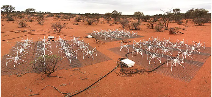
The Square Kilometre Array (SKA) is a new generation radio telescope. It will use data from many antennas distributed over more than 3000 kilometers, to synthesise a new radio telescope with a big collecting area and a very large field of view. However, in this work we used the data from MWA, a precursor of SKA. MWA is a low-frequency radio telescope (it operates between 80 and 300 MHz) and it is located in the desert, in Western Australia. Moreover it is composed by 2048 dual-polarization dipole antennas arranged as 128 tiles (each a 4x4 array of dipoles) with 8128 baselines. The collecting area is about 2000 square meters while the field of view is approximately between 15 and 50 degrees.
The values for the angular resolution are showed in the table 2.1.
The MWA has been used to carry out two surveys of the sky at low frequency. The corresponding catalogues are: the Murchison Widefield Array Commisioning Survey (MWACS) and the GaLactic and Extragalactic All-sky MWA (GLEAM).
Figure 2.1: MWA is located in the australian desert, in the Western Australia baseline frequency angular resolution
1.5 Km 150 MHz ∼ 3 arcmin 3 Km 150 MHz ∼ 2 arcmin 1.5 Km 200 MHz ∼ 2 arcmin 3 Km 200 MHz ∼ 1 arcmin Table 2.1: angular resolution for the MWA.
2.1.1
The Murchison Widefield Array Commisioning
Survey (MWACS)
This survey covers the sky in the region between 0◦≤ RA ≤ 127.5◦ or
307.5◦ ≤ RA ≤ 360◦ and -58.0◦ < Dec < -14.0◦. The observations were
done in October 2012. All the sources of the catalogue have high absolute Galactic latitude and the 3LAC (the catalogue of the F ermi satellite for the blazars) presents object in the same area. So the high Galactic latitude is ideal to study the properties of blazars. The primary work about MWACS is published in Hurley-Walker et al. 2014. The technical features are reported
2.1 A precursor for SKA: the Murchison Widefield Array (MWA) 9
Figure 2.2: Survey of the MWACS with galactic coordinates (Hurley-Walker, et al. 2014). The dark regions are the areas with largest source density.
in the table:
observation band centered at 119, 150, 180 MHz covered area 6100 sq. deg.
number sources 14110 source density 2.31/deg2
sensitivity 50 mJy/beam (from 120-180 MHz) angular resolution ∼ 180 arcsec
Table 2.2: technical features for the MWACS
2.1.2
The GaLactic and Extragalactic All-sky MWA
(GLEAM)
After the completion of MWACS, the MWA was used to carry out a larger and deeper sky survey: the Galactic and Extragalactic All-sky MWA (GLEAM) survey. GLEAM observing began in August 2013 and the first year concluded in July 2014. The second year of observing concluded in July 2015. A third year of observing at high ( 250-310 MHz) frequency concluded in July 2016. The primary work about GLEAM is published in Hurley-Walker et al. 2017.
Figure 2.3: Survey of the GLEAM with galactic coordinates (Hurley-Walker, et al. 2017). The dark regions are the areas with largest source density.
We can see from MWACS to GLEAM both the total number of sources and the surface density grow. In fact with GLEAM we have a larger covered area, a better sensitivity resulting in a larger number of source. In particular the GLEAM survey covered the entire southern sky, except the Magellanic Clouds and Galactic latitude within 10 deg from the Galactic plane.
These catalogues are mainly composed by extra-galactic sources and we expect that GLEAM will improve our knowledge about the low-frequency spectrum of the Active Galactic Nuclei at low and high redshift. Moreover with these data it is possible to research new information about relics and halos in galaxy clusters. Also the investigation for new notions for the cos-mology is a possible field of research. However, in this work we examined the characteristics of blazars. The technical features are reported in the table:
observation band 72-231 MHz covered area 24831 sq. deg. number sources 307455
source density 12.3/deg2
sensitivity 6-10 mJy/beam angular resolution ∼ 100 arcsec Table 2.3: technical features for the GLEAM
2.2 The Very Large Array (VLA) 11
Figure 2.4: The Very Large Array is located in New Mexico, USA.
2.2
The Very Large Array (VLA)
The Very Large Array (VLA) is an interferometer composed by 27 radio antennas in the Plains of San Agustin (80 Km west of Socorro, New Mexico, USA). Every antenna has a diameter of 25 meters. The data of the antennas is combined to obtain the sensitivity of an antenna with a diameter of 130 meters and an angular resolution varying between approximately 0.1” and 45”. We used two catalogues of the VLA: the NRAO VLA SKY SURVEY (NVSS)(Condon et al. 1998) and the Faint Images of the Radio Sky at Twenty (FIRST)(Becker et al. 1995).
2.2.1
The NRAO VLA SKY SURVEY (NVSS)
The NRAO VLA Sky Survey was obtained with the VLA between 1993 September and 1996 October. Other observations were made in the last four months of 1997. The catalogue contains galactic and extra-galactic sources. There are quasars and radio galaxies, most of the galaxies in the IRAS Faint Source Catalog (Moshir et al. 1992), ultra-luminous starburst galaxies even at cosmological distances, low luminosity AGNs, Galactic planetary nebulae, pulsars and stars. The survey covered 82 % of the entire sky. The technical features are reported in the table:
observation band centered at 1.4 GHz covered area 33827 sq. deg. number sources ∼ 1 ×10⁶
source density ∼53/deg2
sensitivity 1.11 mJy/beam angular resolution 45 arcsec Table 2.4: technical features for the NVSS
2.2.2
The Faint Images of the Radio Sky at Twenty
(FIRST)
The First Survey is a project realized using the VLA in the more extended configuration. With this configuration we have a 10 times better angular resolution respect to the configurations of the NVSS. The survey area has been chosen to coincide with that of the Sloan Digital Sky Survey (SDSS) (about 80% of the north sky and 20% south sky). In particular with a limit mv ∼ 23 for the SDSS, about 40% of the counterparts to FIRST objects are
detected.
observation band centered at 1335, 1730 MHz covered area 10000 sq. deg.
number sources ∼ 900000 source density ∼ 90/deg2
sensitivity 1 mJy angular resolution 5 arcsec
2.3 The Australia Telescope Compact Array (ATCA) 13
Figure 2.5: The Australia Telescope Compact Array (ATCA) is located at ∼ 500 km north-west of Sydney, (Australia).
2.3
The Australia Telescope Compact Array
(ATCA)
The Australia Telescope Compact Array is composed by six antennas with a diameter of 22 m and the baselines are 1.5, 3 and 6 Km. It is possible to use the array both at low-frequency (less than 1GHz) and at high frequency (20 GHz). We used a catalogue of the ATCA: the Australia Telescope 20-GHz Survey (AT20G) to study the emission for the AGN at high frequency.
2.3.1
The Australia Telescope 20-GHz Survey (AT20G)
The Australia Telescope 20-GHz Survey (AT20G) is a radio survey at 20 GHz, composed in the period from 2004 to 2008. It covers the whole sky south of declination 0 degrees. It is the largest and most sensitive survey of the sky at this frequency, which is crucial for the study of radio emission from flat-spectrum sources, such as the cores of radio-loud AGNs. The catalogue presents 5890 objects above 20 GHz as well as follow up measurements at 5 and 8 GHz. The technical features are reported in the table:
observation band centered at 5,8,20 GHz covered area 20086 sq. deg. number sources 5890
source density ∼ 0.29/deg2
sensitivity 40 mJy angular resolution 0.15 arcsec Table 2.6: technical features for the AT20G
2.4
The Roma BZCat
The BZCat is a multi-frequency catalog for blazars, and it is regularly updated since the release of the first edition (Massaro et al. 2009). The latest (fifth) edition (Massaro et al. 2015) reports data for 3561 objects. In par-ticular coordinates, redshift and data of different bands (radio, millimetre, optical, X-rays and gamma-rays). All sources are detected at radio wave-length, and the radio data come from other catalogues: NVSS and FIRST at 1.4 GHz and SUMSS at 0.8 GHz. The technical features are reported in the table:
observation band radio (0.8,1.4 GHz), millimetre, optical, X, gamma covered area 41253 sq. deg. (entire sky)
number sources 3561 source density ∼ 0.09/deg2
sensitivity ∼ 1.6 mJy/beam (radio data) angular resolution 5, 45 arcsec, ∼ 1 arcmin (radio data)
2.5 The Sloan Digital Sky Survey (SDSS) 15
2.5
The Sloan Digital Sky Survey (SDSS)
The SDSS catalog contains five-band photometry for 357 million objects. There are over 1.6 million spectra in total 930,000 galaxies, 120,000 quasars and 460,000 stars. This survey is realized to obtain CCD images over 10,000 deg2 of high-latitude sky, and spectroscopy of a million galaxies and 100,000
quasars over the same region. The primary work of this survey is York et al. 2000 and the latest (seventh) edition is released from Abazajian et al. 2009.
observation band 3800-9200 ˚A covered area 11663 sq. deg. number sources ∼ 357 million source density ∼ 30600 /deg2
S/N (signal/noise) 10 per pixel resolution λ/∆λ ∼ 2000
Table 2.8: technical features for the SDSS
2.6
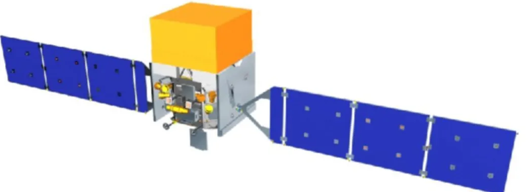
The F ermi satellite
The Gamma-ray Large Area Space Telescope (GLAST), later called F ermi Gamma-ray Space Telescope, is the successor of the Energetic Gamma Ray Experiment Telescope (EGRET), that operated from 1991 to 2000. The satellite was launched on June 11, 2008 on an elliptical orbit at altitude of about 565 Km, with an inclination of 25.6◦ respect to the Earth’s equator (Atwood et al. 2009). F ermi treads the full orbit in about 96 min, also in about 3 hours it scan the entire sky. On board the satellite there are two instruments: the Large Area Telescope (LAT) and the Gamma-ray Burst Monitor (GBM). The LAT is a pair conversion telescope and detects gamma rays between ∼ 20 MeV and ∼ 300 GeV, with a field of view of 2.4 sr, and an
Figure 2.6: rappresentation of the F ermi satellite.
angular resolution < 0.15◦ for E > 10 GeV. F ermi works at high energy of the electromagnetic spectrum, so the strumentation detects individual pho-tons. So about the resolution we must talk about the single photon angular resolution. Infact at high energy every source emits few photons. The LAT presents a tracker, in which gamma rays decay into electron-positron pairs, and a calorimeter, which measures the energy of the pairs. Moreover the ex-ternal surface of the tracker is covered by an anti-coincidence detector. The latter allows to reject cosmic rays. Instead, the GBM is useful to study of transient phenomena between 8 keV and 40 MeV, and it is a complementary instrument while the LAT is the primary instrument on the F ermi satellite. The F ermi project is a work of NASA with the collaboration of Italy, Ger-many, France and Japan.
The mission is an opportunity to examine high energy phenomena from gamma-ray burst, AGN, pulsars, supernova remnants, binary systems and flares from the sun.
2.6.1
The third catalogue of the Fermi-LAT (3FGL)
The third catalogue of the F ermi satellite (3FGL) (Acero et al. 2015) is a catalogue of gamma-ray sources observed by F ermi in the first 4 years of the mission, and it is the successor to the LAT Bright Source List (0FGL), the First F ermi LAT (1FGL) and the Second F ermi LAT (2FGL) catalogues.
2.6 The F ermi satellite 17
The new 3FGL catalog is deeper than the previous catalogues in the 100 MeV-300 GeV energy range. The sources are not distributed evenly. Infact 468 objects are located on the Galactic plane. We reported the features for 3FGL in the table:
observation band 100MeV-300GeV covered area 41253 sq. deg. (entire sky) number sources 3033
source density 0.07/deg2
Table 2.9: technical features for the 3FGL. We can see that the source density is very low compared to the source density in the radio surveys
energy value per-photon angular resolution 100 MeV ∼ 5◦
1 GeV 0.8◦ above 20 GeV ∼ 0.2◦
Table 2.10: angular resolution for the 3FGL. The resolution rises to the drop in energy. Infact the resolution varying with energy approximately as E−0.8.
The third LAT AGN Catalogue (3LAC)
Most of the 3FGL sources are blazars, and these objects compose a subset of the 3FGL: the 3LAC. Infact the 3LAC sources are identified with AGNs. The catalogue contains accurate positions for the low frequency counterparts and information about the multiwavelength properties: redshift, radio, opti-cal and X-ray flux, position of the peak of the synchrotron component of the Spectral Energy Distribution (SED). In particular the subset is composed by 680 Low Synchrotron Peaked (LSP), 296 Intermediate Synchrotron Peaked (ISP), 393 Low Synchrotron Peaked (LSP), sources in according to the SED
Figure 2.7: Survey of the 3LAC with galactic coordinates (Ackermann, et al. 2015).
classification; and it presents 414 Flat-Spectrum Radio Quasar (FSRQ), 604 BL Lacertae (BL Lacs) and 402 Blazar Candidate Unidentified (BCU), and the latter are blazars but we are not sure about which kind of blazar.
Redshift distribution
Let us consider the redshift distribution of these objects. The LSP and FSRQ are at larger redshift then other sources. This suggests that many LSP are FSRQ. Also we must consider many BL Lacs have not a value for the redshift so it is not possible to report all objects in a redshift distribution. However, in the 3LAC we have objects with a redshift in the range between 3.104 and 0.0018 so we see sources both high and low redshift.
In the figure 2.8 we see the redshift distributions for FSRQs, BL Lacs and BCUs. There are sources of the 3LAC and of the 2LAC. The latter is the Second Catalog of Active Galactic Nuclei detected by F ermi and it is the previous catalog of the 3LAC. For the FSRQs the distribution of the 3LAC sources and the distribution of the 2LAC sources are similar. The two dis-tributions show that the number density of FSRQs grows drammatically up to redshift z ∼ 0.5-2.0. For z < 2 the two distributions decline (Ajello et al. 2012).
Also for the BL Lacs the distribution of the 3LAC sources and the distri-bution of 2LAC sources are similar, with a maximum near z=0.3. In the
2.6 The F ermi satellite 19
Figure 2.8: redshift distributions (solid: 2LAC sources; dashed: new 3LAC sources) for FSRQs (top), BL Lacs (middle), and different types of BL Lacs (bottom): LSPs (green), ISPs (light blue), and HSPs (dark blue). The ranges between the lower and upper limits are also depicted in the bottom panel when both limits are available (Ackermann et al. 2015).
figure there are different kinds of BL Lac: LSP, ISP and HSP. The redshift distributions gradually spread out to higher redshifts from HSP-BL Lacs to LSP-BL Lacs.
Flux and photon spectral index
The Fig. 2.9 shows the photon index distributions for different blazars classes (FSRQs, BL Lacs, BCUs). The distributions report the sources of the 2LAC and the 3LAC. The sources detected in the 3LAC are slightly softer than the 2LAC sources. In other words, with the new catalog it is possible to detect lower energy peaked blazars. Instead, there is no differences for the two samples of BL Lacs. For the BCUs the distribution of the 3LAC extends at larger values for the photon spectral index. Also we see the FSRQs present a larger photon spectral index than the BL Lacs.
Figure 2.9: Photon spectral index distributions. Top: FSRQs (solid: 2LAC sources; dashed: new 3LAC sources). Second from top: BL Lacs (solid: 2LAC sources; dashed: new 3LAC sources). Third from top: 3LAC LSP-BL Lacs (green), ISP-LSP-BL Lacs (light blue), and HSP-LSP-BL Lacs (dark blue). Bottom: blazars of unknown type (solid: 2LAC sources; dashed: new 3LAC sources) (Ackermann et al. 2015).
The Fig. 2.10 shows the photon index versus the photon flux with the de-tection limit. In particular the dede-tection limit of the 3FGL (solid line) is better than the detection limit of the 2FGL (the Second Catalog of F ermi and previous catalog of the 3FGL). Also in this figure we can see that the FSRQs are the objects with the largest photon index.
2.6 The F ermi satellite 21
Figure 2.10: Photon spectral index vs. photon flux above 100 MeV for blazars in the 3LAC Sample. Red circles: FSRQs; blue circles: BL Lacs; green triangles: blazars of unknown type; magenta stars: other AGNs. The solid (dashed) curve represents the approximate 3FGL (2FGL) detection limit based on a typical exposure. The 2FGL is the second catalog of F ermi while the 3FGL is the third catalog (Ackermann et al. 2015).
Chapter 3
Cross-correlations of catalogues
In this chapter we report all cross-correlations of the catalogues executed in this work.
The new low-frequency radio data are opening a new window for the study of the sky, especially for the blazars. These objects are so poorly studied at low frequency and now we can better characterize known source classes. In a previous work (Giroletti et al. 2016), the authors cross-correlated the 6100 deg2of the MWACS with the sources of the BZCat and the 3LAC. They
found low frequency counterparts for 186 out of 517 (36%) blazars, 79 out of 174 (45%) gamma-ray blazars. The limited detection rate caused a selection bias. Infact the lower sources (especially BL Lacs) were under-represented. Similar biases affected earlier works by Massaro et al. 2013 and Nori et al. 2014. In this thesis we cross-correlated the 24831 deg2 of the GLEAM with the 3LAC. So we have a larger number of data to analyse. Infact we showed in the chapter 2 the properties for GLEAM and MWACS, and we know with GLEAM, we have a deeper survey, with more sources, a better sensitivity and less affected by selection bias. In other words, this is the first time that the spectral properties of blazars at low frequency can be discussed with a large and representative data sets.
Also we done also cross-correlations for other catalogues that we report in this chapter.
3.1
Cross-correlation for the GLEAM and the
3LAC
We cross-matched the two catalogues, using a positional uncertainty of 1” for the 3LAC sources and the uncertainty reported in the catalogue for GLEAM. The value of 1” for the error of the 3LAC is a reasonable estimate, considering the values for the errors of the catalogues which contain the coun-terparts at radio frequency of the gamma-ray sources. Infact in the 3LAC, the radio counterparts come from different surveys: AT20G, NVSS, SUMSS, FIRST and PMN surveys. Every survey presents a particular angular reso-lution and a particular frequency. So in every survey there is a value for the error, and the latter is different comparated another error of another survey. Moreover, the most blazars selected are calibrators for the VLBI (Very Large Baseline Interferometry), and their position is known with an uncertainty of the order of the milliarcosecond, so 1” is very conservative choice. Anyway more information are reported in Ackermann et al. 2015.
Therefore from the 307455 sources in the GLEAM and from the 1444 sources in the 3LAC (963 in the GLEAM sky), we obtained 747 matches (blazars): 424 LSP, 131 ISP, 165 HSP for the SED classification, and 267 FSRQ, 257 BL LACS, 214 BCU for the spectroscopic classification. Also 747 objects is an high detection rate, infact we estimated 963 gamma-ray sources in the sky of the GLEAM. In other words, the most blazars are detected at low frequency.
Moreover, we created a false 3LAC with inverted declination, to verify the correct efficiency of the cross-correlation between the GLEAM and the 3LAC. So we cross-correlated the false 3LAC with the GLEAM and we obtained 75 matches. This number is much smaller than 747 (number of the matches for the true 3LAC), infact this means that the fraction of spurious matches in our cross-correlation is about 10%. Therefore we concluded that we exe-cuted a good cross-correlation because the matches are right. Moreover the 3LAC have not the gamma fluxes, unlike the 3FGL. So we cross-correlated
3.2 Cross-correlation for the AT20G and the 3LAC 25
Figure 3.1: Survey of the blazars with a counterpart at low-frequency (3LAC vs. GLEAM). Obviously the sources are in the sky area of the GLEAM survey.
the two catalogues to obtain the gamma flux for the 3LAC sources. We cross-correlated the two samples, identifying the matches with the sources with the same name.
3.2
Cross-correlation for the AT20G and the
3LAC
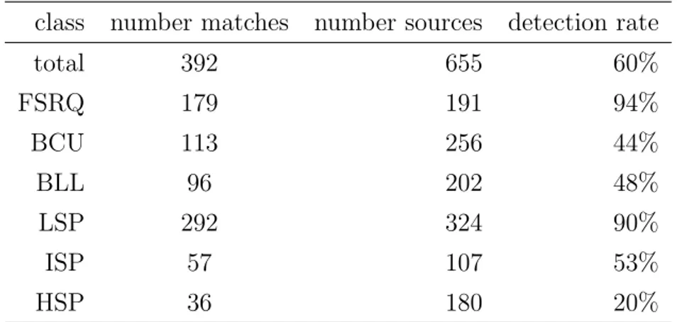
We cross-correlated the 3LAC with the AT20G. The former present 1444 sources and the latter contains 5890 sources and with the cross-correlation we obtained 392 matches. So these sources are selected blazars at high fre-quency. This selection is useful to study the emission from the core of the radio sources. However, analyzing the position of the synchrotron peak, these sources are 292 LSP, 57 ISP, 36 HSP. Instead for the spectroscopic classifi-cation they are 179 FSRQs, 96 BL Lacs, 113 BCUs.
Figure 3.2: Survey of the detected blazars at high frequency (3LAC vs. AT20G). The most objects are in the Southern sky. Infact the most sources of the AT20G are in the same sky.
3.3
Cross-correlation for the AT20G and the
GLEAM
We remember that the AT20G has 5890 objects and the GLEAM has 307455 objects.
This cross-matches are done using the same algorithm of the previous sec-tions. In other words, we obtained some radio sources at low and high fre-quency. The number of the matches is 4271. The cross-correlation represents a method to compare the core emission (at high frequency) and the extended emission (at low frequency). In particular if we estimate the ratio between SAT20G and SGLEAM, we expect that a core dominated source (like a blazar)
will have a larger ratio than a lobe dominated source (like a radio-galaxy). In the next chapters we will show this behaviour. Moreover, the AT20G catalogue have not a spectroscopic classification, so we obtained the optical counterparts from Mahony et al. 2011. Therefore we cross-matched the op-tical catalogue (composed by 5890 objects) with the AT20G, identifying the matches with the objects with the same name.
3.4 Cross-correlation for the 3LAC and AT20G-GLEAM 27
Figure 3.3: Survey for radio sources at low and high frequency (AT20G vs. GLEAM).
Figure 3.4: Survey for blazars selected at low and high frequency (3LAC vs. AT20G-GLEAM).
3.4
Cross-correlation for the 3LAC and
AT20G-GLEAM
We cross-correlated the 3LAC with the generated catalogue from the cross-correlation between AT20G (5890 sources) and GLEAM (307455 sources). Therefore, we created a survey with 208 gamma-ray blazars at low and high frequency: 171 LSPs, 16 ISPs, 21 HSPs and 151 FSRQs, 36 BL Lacs, 19 BCUs.
Figure 3.5: Survey radio sources at low and intermediate frequency (BZCat vs. GLEAM).
3.5
Cross-correlation for the BZCat and GLEAM
We cross-correlated the 3561 sources of the BZCat with the 307455 sources of GLEAM, using the usual method, and we extracted 1709 matches: 1122 FSRQs, 442 BL LACs and 141 BCUs. We have not a classification for the position of the synchrotron peak in the sample. In general, in a sample the LSPs and the FSRQs are the most objects of the entire population, and in this catalogue we can see that the FSRQs rappresent a very large number compared to the other classes. This suggests that the FSRQs are brightest.
3.6
Cross-correlation 3LAC-GLEAM and
BZCat-GLEAM
In the previous sections we described the cross-correlations 3LAC-GLEAM and BZCat-GLEAM. Then we cross-correlated the two catalogues obtained. For the sample 3LAC-GLEAM we have 747 sources and for the sample BZCat-GLEAM we have 1709 sources. Therefore, executing this cross-match, we selected blazars at low and intermediate frequency. The new sample coin-tains 530 sources: 331 LSPs, 88 ISPs, 106 HSPs and 239 FSRQs, 248 BL Lacs, 40 BCUs. We see that the number of BL Lacs is larger than the num-ber of FSRQs. In general the opposite is true. Anyway we must consider that
3.7 Anticross-correlation BZCat-GLEAM and 3LAC-GLEAM 29
Figure 3.6: Survey for the blazars selected at low and intermediate frequency (3LAC-GLEAM vs. BZCat-GLEAM).
we have 40 candidate blazars, and we do not know which kind of blazars they are. It needs to be noted that in the 3LAC there are many sources that are classified as blazar candidates on the basis of their multi-wavelength proper-ties, yet they lack spectroscopic information. As such, they are not confirmed blazars and they do not appear in the BZCat master list. Indeed they form the bulk of the 747-530=217 sources missed in this cross-correlation.
3.7
Anticross-correlation BZCat-GLEAM and
3LAC-GLEAM
We executed an anticross-match between BZCat-GLEAM (1709 objects) and 3LAC-GLEAM (747 objects). So we obtained a sample composed by 1179 objects with 883 FSRQs, 193 BL Lacs, 101 BCUs. These are blazars that are detected by GLEAM but not by F ermi. We have not the SED classification for these sources.
Figure 3.7: Survey for the anticross-correlation BZCat-GLEAM and 3LAC-GLEAM.
Figure 3.8: Survey of radio sources selected at low and intermediate frequency (SDSS, FIRST, NVSS, GLEAM).
3.8
Cross-correlation for SDSS-FIRST-NVSS
and GLEAM
The SDSS-FIRST-NVSS (18286 objects) (Best et al. 2011) is a sample with the combined data from SDSS, FISRT and NVSS. We cross-correlated this catalogue with the GLEAM (307455 objects). With this cross-correlation we achieved 2906 sources. We divided the sample in three populations: ob-jects with the flux density of the FIRST SFIRST = 0, with the density flux of
the FIRST SFIRST 6= 0, and the sources of the radio-class 1. We will explain
3.9 Cross-correlation 3LAC-GLEAM and 3LAC-AT20G 31
Figure 3.9: Survey of blazars detected at low and high frequency (3LAC-GLEAM vs. 3LAC-AT20G).
3.9
Cross-correlation GLEAM and
3LAC-AT20G
We cross-correlated the sample of the blazars detected at low frequency (3LAC-GLEAM), composed by 747 objects, with the sample of the blazars detected at high frequency (3LAC-AT20G), composed by 392 objects. There-fore we generated a sample with 367 objects. We will use this new sample to study the nuclear properties of blazars in Chapter 5.
3.10
Statistics
In this section we report a summary to describe the statistical data about the samples generated. We do not report the statistical data for the cross-correlation between the GLEAM with the 3LAC: we will report these data in the next chapter.
With the cross-correlation 3LAC vs. AT20G we see the blazars detected at high frequency, and we can see that the most blazars are detected at low frequency.
The detection rate for the cross-match AT20G vs. GLEAM is high (88%), so in the most cases if a blazar emits at low frequency it also emits at high frequency.
While for the cross-correlation 3LAC vs. GLEAM-AT20G the detection rate is not so high (only 31%), so the blazars detected both at high and low fre-quency are not many objects.
The BZCat is the most complete catalog for blazars in the literature, and the most blazars of this catalog are detected at low frequency, infact the detection rate for the cross-match BZCat vs. GLEAM is 76%.
In the cross-correlation 3LAC-GLEAM vs. BZCAT-GLEAM we estimated the number of blazars of the BZCat detected at low frequency are detected at high energies (gamma-rays). The detection rate (71%) suggest a correlation between gamma emission and radio emission. However we will explain this relation in the chapter 4.
The cross-correlation FIRST-SDSS-NVSS vs. GLEAM is a comparison be-tween low and intermediate frequency and the detecton rate is not high (only 26%). Anyway we must consider that the presence of differents angular res-olutions for many catalogues.
The cross-match 3LAC-GLEAM vs. 3LAC-AT20G presents blazars at high and low frequency, and the detection rate is close to half of the entire sample selected (49%).
class number matches number sources detection rate
total 392 655 60% FSRQ 179 191 94% BCU 113 256 44% BLL 96 202 48% LSP 292 324 90% ISP 57 107 53% HSP 36 180 20%
3.10 Statistics 33
class number matches number sources detection rate total 4271 4858 88%
Table 3.2: statistical data for the cross-match AT20G vs. GLEAM. We have not data for SED and spectroscopic classifications.
class number matches number sources detection rate
total 208 665 31% FSRQ 151 192 79% BCU 19 259 7% BLL 36 207 17% LSP 171 330 52% ISP 16 109 15% HSP 21 182 12%
Table 3.3: Statistical data for the cross-match 3LAC vs. AT20G-GLEAM
class number matches number sources detection rate total 1709 2238 76%
FSRQ 1122 1272 88%
BCU 141 189 75%
BLL 442 777 57%
Table 3.4: statistical data for the cross-match BZCat vs. GLEAM. We have not data for SED and spectroscopic classifications.
class number matches number sources detection rate total 530 747 71% FSRQ 239 267 90% BCU 40 214 19% BLL 248 257 96% LSP 331 424 78% ISP 88 131 67% HSP 106 165 64%
Table 3.5: statistical data for the cross-match 3LAC-GLEAM vs. BZCat-GLEAM
class number matches number sources detection rate total 2906 11112 26%
Table 3.6: statistical data for the cross-match SDSS-FIRST-NVSS vs. GLEAM. We have not data for SED and spectroscopic classifications.
class number matches number sources detection rate
total 367 747 49%
Table 3.7: statistical data for the cross-match GLEAM vs. 3LAC-AT20G. We have not data for SED and spectroscopic classifications.
Chapter 4
Results about the spectral
properties for blazars detected
at low frequency
4.1
Detection rate: a jump from MWACS to
GLEAM
In the previous chapter we reported on a previous work (Giroletti et al. 2016) where some gamma-ray blazars are detected at low frequency with MWACS. With the GLEAM the detection rate grows to 78%, compared to 45% found in MWACS. Also the detection rate grows for every kind of ob-jects, both considering the SED and spectroscopic classification. The growth of the detection rate is impressive, in particular for the faintest classes, such as BL Lacs, which raises from 22% in MWACS to 71% in GLEAM. However, the largest group of sources remains that of LSP, both because there are many of them in the starting sample (3LAC) and because the detection rate is larger. We reported the results in the Table 4.1. We see that the number of the LSP is larger than the number of the ISP and the HSP. Infact, the former have the largest detection rate for the SED classification. Also the
number of the ISP is lower than the number of the HSP, but the latter have a lower detection rate. For the spectroscopic classification the FSRQs have the largest detection rate, instead the detection rates for the BL Lacs and the BCUs are similar. The Figures 4.1 and 4.2 give us an idea about the detection rate as a function of the ∼ GHz flux density (Fig. 4.1) and the gamma-ray energy flux (Fig. 4.2). Infact in these figures we compared the 3LAC sample with the GLEAM sample. We can see that the detection rate grows for brighter objects, both in the radio band and in the gamma band. The two distributions do not have the exact same shape. The starting gamma-ray energy distribution has the typical features of the source count distribution for a complete sample: the source counts increase regularly as the flux decreases, and then they suddenly turn over as the limiting sensitiv-ity is reached; the brightest gamma-ray sources nearly always have a GLEAM match, and then the GLEAM detection rate decreases for fainter sources.
The radio distributions are much more symmetric, without a well defined turn over at low flux density. An interesting feature is the rather large number of gamma-ray blazars with GHz radio flux density larger than the GLEAM sensitivity (6-10 mJy) but not detected in our match. These sources must have an inverted spectrum.
4.1.1
Multi-wavelength and spectral statistical
prop-erties
In this section we report the results about the values for the mean flux (in X, gamma and radio band) and the spectral index. So we show the spectral properties through the numbers. We reported the mean values in the Table 4.2. We can see some properties that we will discuss also in the next section: in the radio band the LSP are brighter than the HSP, while in the X-ray band the latter are brighter than the former. In the gamma band we have the same behaviour of the radio band for the HSP and LSP. Instead, the ISP have intermediate value of the flux in every band. Also the FSRQs are
4.1 Detection rate: a jump from MWACS to GLEAM 37
Figure 4.1: radio flux density at 1GHz distribution for the entire 3LAC sam-ple (red) in the GLEAM sky and 3LAC sources with a GLEAM counterpart (blue).
Figure 4.2: gamma-ray flux at E > 100 MeV distribution for the entire 3LAC sample (red) in the GLEAM sky and 3LAC sources with a GLEAM counterpart (blue).
class ratio detection rate for GLEAM ratio detection rate for MWACS total 747/963 78% 87/247 35% FSRQ 267/278 96% 52/71 73% BCU 214/312 69% 16/89 18% BLL 257/362 71% 19/87 22% LSP 424/460 92% 67/128 52% ISP 131/179 73% 11/37 30% HSP 165/270 61% 9/68 13%
Table 4.1: The detection rate from MWACS to GLEAM grows for every kind of object.
brighter than the BL Lacs in the radio and gamma band. In the X-ray band the BL Lacs are brighter than the FSRQs. In the radio and X-ray band the BCUs have intermediate value of the flux; instead in the gamma band they are the objects with the lowest flux. The Figure 4.3 is a flux density distribution at low frequency, and show that blazars are brighter than the rest of GLEAM sources.
Moreover we reported in the Table 4.3 the mean values of the spectral index. We note that the GLEAM catalogue does not report a spectral index for all sources, since some of them have complex spectra difficult to fit with a power law. Therefore, we write the total number of sources (detected at low frequency) and the number of the sources with the value for spectral index for every class. Analyzing the values of the spectral index, we see that the LSP seem have a slightly flatter spectrum than the HSP (∆α = αLSP− αHSP =
0.23). So, at first sight, the LSP are closer to a core dominated object and they are closer to a lobe dominated object. This is an intriguing result. Infact, before we expected every blazar to have about the same value of the spectral index, instead now we see different values for HSP and LSP. Also we observe a similar difference between BL Lacs and FSRQs, yet quantitatively less significant (∆α = 0.06).
4.1 Detection rate: a jump from MWACS to GLEAM 39
Moreover, the mean value of the spectral index for all objects in the GLEAM is < α >= −0.77, while the value for the object reported both in the GLEAM and in the 3LAC is < α >= −0.45. Also we reported a distribution for the spectral index (Fig. 4.4) that show this behaviour. This result is of great interest: while it is well known that blazars have flat spectra at high frequency, it has only recently started to become clear that they maintain a flat spectrum down to low frequency (Massaro et al. 2013, Nori et al. 2014). Our result indicates that the flat spectrum cores still contribute a substantial fraction of the radio emission in the ∼ 100 MHz regime. We will estimate this fraction in a later section of this work. This distribution is an interesting test for the Unified Model for AGN. Infact for this model the objects with a larger spectral index are core dominated and the objects with a lower spectral index are lobe dominated.
class log Frad [mJy] log FX [10−13erg/cm2/s] log Fγ [erg/cm2/s]
total 2.4 ±0.6 1.5 ±0.6 -11.0 ±0.4 FSRQ 2.8 ±0.4 1.2 ±0.4 -10.9 ±0.4 BCU 2.2 ±0.5 1.4 ±0.5 -11.2 ±0.3 BLL 2.2 ±0.5 1.7 ±0.6 -11.0 ±0.4 LSP 2.7 ±0.5 1.2 ±0.4 -10.9 ±0.4 ISP 2.3 ±0.5 1.2 ±0.4 -11.1 ±0.4 HSP 1.9 ±0.4 1.8 ±0.5 -11.1 ±0.4 Table 4.2: values for the logarithm of the radio (∼ 1GHz) flux density Frad,
X-ray flux FXand gamma-ray flux Fγ. The associated errors are the standard
Figure 4.3: normalized flux density distribution at low frequency for all GLEAM sources (green) and low frequency detected blazars (blue). Blazars are brighter then the rest of GLEAM sources.
Figure 4.4: normalized spectral index distribution for the blazars detected at low frequency (blue) and all GLEAM sources (green). The blazars are flatter-spectrum objects than the rest of the sample.