Roberto Terzano*, Melissa A. Denecke, Gerald Falkenberg, Bradley Miller, David
Paterson and Koen Janssens
Recent advances in analysis of trace elements
in environmental samples by X-ray based
techniques (IUPAC Technical Report)
https://doi.org/10.1515/pac-2018-0605Received June 21, 2018; accepted March 13, 2019
Abstract: Trace elements analysis is a fundamental challenge in environmental sciences. Scientists measure trace elements in environmental media in order to assess the quality and safety of ecosystems and to quantify the burden of anthropogenic pollution. Among the available analytical techniques, X-ray based methods are particularly powerful, as they can quantify trace elements in situ. Chemical extraction is not required, as is the case for many other analytical techniques. In the last few years, the potential for X-ray techniques to be applied in the environmental sciences has dramatically increased due to developments in laboratory instru-ments and synchrotron radiation facilities with improved sensitivity and spatial resolution. In this report, we summarize the principles of the X-ray based analytical techniques most frequently employed to study trace elements in environmental samples. We report on the most recent developments in laboratory and synchro-tron techniques, as well as advances in instrumentation, with a special attention on X-ray sources, detectors, and optics. Lastly, we inform readers on recent applications of X-ray based analysis to different environmen-tal matrices, such as soil, sediments, waters, wastes, living organisms, geological samples, and atmospheric particulate, and we report examples of sample preparation.
Keywords: environment; plants; sediments; soil; synchrotron; trace elements; wastes; XAS; XCMT; X-rays; XRD; XRF.
CONTENTS
1 INTrOduCTION ������������������������������������������������������������������������������������������������������������������������� 1030 2 BaSIC PrINCIPlES ���������������������������������������������������������������������������������������������������������������������1032 2.1 X-ray physics ... 1032 2.2 X-ray fluorescence analysis and related methods ...1033 2.3 Microscopic elemental analysis: μ-XRF, EPMA/SEM-EDX and μ-PIXE ...1034
Article note: Sponsoring body: IUPAC Chemistry and the Environment Division: see more details on page 1058.
*Corresponding author: Roberto Terzano, Department of Soil, Plant and Food Sciences, University of Bari, Via Amendola 165/A,
70126 Bari, Italy, e-mail: [email protected]
Melissa A. Denecke: The University of Manchester, Dalton Nuclear Institute, Oxford Road, Manchester M14 9PL, UK Gerald Falkenberg: Deutsches Elektronen-Synchrotron DESY, Photon Science, Notkestr. 85, 22603 Hamburg, Germany
Bradley Miller: United States Environmental Protection Agency, National Enforcement Investigations Center, Lakewood, Denver,
CO 80225, USA
David Paterson: Australian Synchrotron, ANSTO Clayton Campus, Clayton, Victoria 3168, Australia
2.4 Quantitative aspects of X-ray analyses ...1035
2.5 X-ray absorption spectroscopy ...1035
2.6 X-ray diffraction ...1038
2.7 X-ray Micro Tomography ...1039
2.8 X-ray sources, optics and detectors ... 1040
2.8.1 Laboratory sources ... 1040
2.8.2 Synchrotron X-ray sources ... 1040
2.8.3 X-ray microfocussing optics ... 1041
2.8.4 X-ray detectors and cameras ... 1041
3 SyNChrOTrON TEChNIquES aNd INSTrumENTaTION ��������������������������������������������������������� 1042 3.1 Relevant synchrotron-based imaging techniques ...1042
3.1.1 X-ray Fluorescence Microscopy...1043
3.1.2 Spatially resolved X-ray Absorption Spectroscopy ...1043
3.1.3 X-ray fluorescence tomography and confocal detection ...1044
3.2 Types of samples that can be analysed...1045
3.3 General overview of instruments and facilities ...1046
4 aPPlICaTIONS TO ENvIrONmENTal SamPlES ����������������������������������������������������������������������1046 4.1 Soil ...1046
4.2 Rocks ...1047
4.3 Waters and sediments ...1049
4.4 Plants ... 1051
4.5 Other living organisms ... 1053
4.6 Wastes ...1054
4.7 Nuclear wastes ...1054
4.8 Atmospheric particulate ...1056 5 CONCluSIONS aNd PErSPECTIvES �������������������������������������������������������������������������������������������1057 aBBrEvIaTIONS ������������������������������������������������������������������������������������������������������������������������ 1058 aCkNOwlEdgEmENTS ������������������������������������������������������������������������������������������������������������� 1058 mEmBErShIP OF ThE SPONSOrINg BOdy ������������������������������������������������������������������������������������� 1058 rEFErENCES ����������������������������������������������������������������������������������������������������������������������������������� 1059
1 Introduction
X-ray based techniques for elemental analyses have advanced dramatically over the last two decades. The use of X-ray based techniques has expanded into a wide variety of scientific disciplines. These include the materials sciences, including metallurgy and mineralogy [1]; the environmental sciences, such as soil and water chemistry [2]; as well as the biological sciences [3–5]. The recent development and availability of X-ray based techniques, in particular those making use of synchrotron light sources, have significantly increased our understanding of the role of trace elements in the environment and in living organisms.
Trace elements, trace metal(loid)s, minor elements, and micronutrients are terms used in a number of sciences and the terms have some commonality. Historically, geologists considered trace elements to be “all elements except the eight abundant rock-forming elements: oxygen, silicon, aluminium, iron, calcium, sodium, potassium, and magnesium” [6]. Therefore, elements at concentrations of 0.1 % and lower were considered trace elements. The IUPAC Gold Book defines trace elements as “Any element having an average concentration of less than about 100 parts per million atoms” [7].
Trace elements in environmental matrices can be studied with a wide array of analytical techniques. These are usually selected based on the aggregation state of the sample (solid, liquid, gas), the element(s) to be detected and their concentration, the degree of heterogeneity of the samples, the purpose of the study, and the available instrumentation. In this report, only analytical techniques employing X-rays, both as primary
scientists and stakeholders to determine the beneficial and detrimental fate and transport of trace elements in organisms and the environment.
X-rays are electromagnetic radiation with a wavelength between 10−11 and 10−8 m, corresponding to
ener-gies between 100 keV and 100 eV. Because of their short wavelength (comparable to the size of atoms) and high energy, they can penetrate tens to hundreds of micrometers into most materials and give rise to a number of physical phenomena that allow the determination of their chemical composition and structure.
For example, when X-rays impinge on a sample, elastic scattering in the form of single-crystal diffrac-tion, powder diffracdiffrac-tion, or coherent diffraction reveals atomic structure information and can be measured by X-ray-sensitive detectors. Inelastic scattering can be observed by either energy or wavelength dispersive detectors to determine the elemental composition and chemistry. X-ray absorption spectroscopy can be used to determine nearest-neighbour atoms structures and local chemistry. In addition, the penetrating power of X-rays allows for studies in three dimensions (3D) without physical sample sectioning or similar disruptive operations and is a key factor in several environmental studies [8].
Four main distinctive features characterize X-ray-based analytical methods: i) non- to minimally-destructive nature, ii) multi-elemental capability, iii) limited or no sample preparation requirement, and iv) spatially-resolved (in both two (2D) and three dimensions (3D)) analyses. These features allow X-ray based techniques to meet the complex needs of modern environmental scientists in studying trace elements in complex heterogeneous environmental media, under in situ conditions and at environmentally relevant concentrations [9, 10].
A number of X-ray based techniques are now available in many laboratories around the world, both as equipment built in-house and as commercial instruments. Limitations in sensitivity can be overcome in some cases by the use of high flux synchrotron sources. The continuous improvement of synchrotron light sources and X-ray beamlines has allowed for the investigation of extremely dilute elements in complex envi-ronmental samples around the world. Recently some of the most original envienvi-ronmental research studies have been significantly enhanced by incorporating synchrotron radiation-based X-ray technique(s) [11]. The high brightness of synchrotron sources may increase the risk of radiation damage occurring, especially in biological samples and organic compounds [12]. In addition, as demand for access to synchrotron techniques by environmental scientists continues to rise, it is becoming increasingly difficult to obtain beamtime at these facilities. Significant developments have been introduced in laboratory instruments which permit basic X-ray analyses on environmental samples.
Among their applications, X-ray techniques gave a remarkable contribution to the understanding of the biogeochemistry of nutrient and contaminant elements in environmental media, as well as their specia-tion and behaviour under different condispecia-tions and at multiple length scales. An important feature of X-ray methods is the possibility to integrate spectroscopic analyses at multiple length scales, from the millimetre to the submicron size, allowing the investigation of trace elements in highly heterogeneous environmental media where inorganic and organic compounds coexist with biota, water, and air, such as in soils and sedi-ments [11, 13].
In recent years, third generation synchrotrons and X-ray free electron lasers capable of measuring femto-second reactions have expanded our knowledge of fundamental chemical events, such as electron transfer, bond breaking/formation, and excited-state formations [14]. Understanding fundamental chemistry has real world consequences, for example, improving the manufacturing and efficiencies of materials (e.g. solar cells) affected by trace element impurities [15]. Synchrotron-based technologies are constantly being improved and will continue to elucidate the chemistry of life and environment.
In this report, following a brief description of the basic principles of the most common X-ray based techniques, a survey of both laboratory and synchrotron instruments will be presented, including their applications to different types of environmental matrices, such as air, water, soil, sediments, plants, living organisms, geological samples, and wastes. X-ray based imaging (2D and 3D) and microscopy techniques are also described and compared.
2 Basic principles
2.1 X-ray physics
The main analytical methods that make use of X-rays [16] discussed in this paper are X-ray fluorescence analysis (XRF), X-ray diffraction (XRD), and X-ray absorption spectroscopy (XAS). In addition, the use of X-ray computed microtomography (XCMT) for investigation of the 3D structure of materials is addressed.
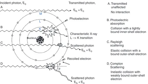
XRF, XAS, and XCMT are based on the photo-electric effect, i.e. the absorption of an impinging X-ray photon by an atom, giving rise to the emission of a photo-electron that leaves an (inner) shell vacancy behind. Secondary processes that fill the vacancy are electronic transitions, some of which result in the emission of characteristic X-rays called fluorescence (depending on the core vacancy and Z of the element). This is illus-trated in Fig. 1 as process B. In the primary energy (E0) range from 10–100 keV, the photo-electric effect is the most important type of interaction between X-rays and matter. Figure 1 also depicts the alternative ways in which X-rays may interact with matter. Process A corresponds to the unhindered passage of the primary X-ray photon, i.e. transmission. Process C, called Rayleigh scattering, is the result of the coherent interaction of the totality of the electrons in the atom with the X-ray photon. It involves a change in direction of the original wave, while its energy/wavelength is conserved (elastic scattering). X-ray diffraction results from the interfer-ence of Rayleigh-scattered X-rays of periodically spaced atoms. In process D, called Compton scattering, a single (weakly bound) electron exchanges energy and momentum with the impinging photon, causing it to become ejected from the atom as a recoil electron. This process changes the direction and energy of the X-ray photon; its final energy (Es) depends on the scattering angle θ.
The relative magnitude of processes B−D is expressed by their respective cross sections σphoto-el., σCoherent, and σIncoherent, the sum of which, multiplied by the ratio of the Avogadro constant (NA ≈ 6.02252 × 10²³ mol−1) and
the molar mass M of the material (in g/mol), is called the mass attenuation coefficient μm = (σphoto-el. + σCoherent + σIncoherent) NA/M, which is a quantity that depends on both the atomic number and the photon energy. The mass attenuation coefficient of a multi-element material is given by μm = Σi wi μmi, where μmi is the mass attenuation coefficient of the ith elemental constituent and w
i its mass fraction. The transmitted intensity It of a beam of
monochromatic X-rays through a foil of a material of thickness d and density ρ is given by Beer’s law:
0 0
exp[ ( ) ]
t m
I = I −μ E ρd (1)
where I0 is the original intensity of the beam with energy E0. The product μm · ρ is called the linear attenuation coefficient (μ).
Incident photon, E0 A
Nucleus
Photoelectron
Transmitted photon, A. Transmitted unaffected B. Photoelectric absorption C. Rayleigh scattering D. Compton Scattering
Collision with a tightly bound inner-shell electron
Elastic collision with a bound outer-shell electron
Inelastic collision with weakly bound outer-shell electron Characteristic X-ray L –> K transition Scattered photon Recoiled electron φ θ Scattered photon ER = E0 ER = E0 ES < E0 B M L K C D No interaction
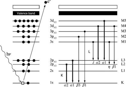
XRF analysis is a powerful analytical tool for the spectrochemical determination of many of the elements present in a sample [17]. The emission of element-specific characteristic radiation, X-ray fluorescence, is induced when photons of sufficiently high energy remove inner shell electrons from their atom by the photoelectric effect, creating electron vacancies in inner shells (K, L, M, …; see Fig. 2). The creation of a vacancy in a particular shell results in de-excitation within 100 fs via a cascade of electron transitions, cor-related with the emission of secondary (X-ray) photons and secondary electrons. The emitted photons have a well-defined energy corresponding to the difference in energy between the atomic shells involved. Not all relaxation transitions of electrons from outer shells or subshells to the core vacancy are allowed, only those obeying the selection rules for electric dipole radiation. The family of characteristic X-rays, corresponding to the element’s transitions, allows the identification of the element. Next to this radiative form of relaxation, a competing process involves the emission of secondary electrons. In this process, the core vacancy is filled by electrons from higher atomic shells, but instead of emitting secondary photons, the transition energy asso-ciated with this relaxing electron is imparted to another electron, which is then itself emitted. This emitted secondary electron is called an Auger electron. This process will not be discussed further here.
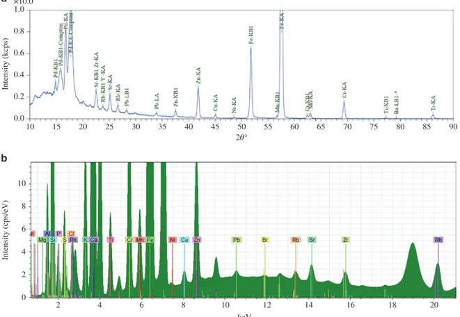
XRF analysis is achieved through the measurement of wavelength or energy and intensity of the charac-teristic photons emitted from a sample. This allows the identification of the elements present in the sample and the determination of their mass or concentration. All the information for the analysis is stored in the measured spectrum, which is a line spectrum with all characteristic lines superimposed above a certain fluc-tuating background (Fig. 3). Other interaction processes, mainly the elastic and inelastic scattering of the primary radiation on sample and substrate, contribute to the background.
Measurement of the spectrum of the emitted characteristic fluorescence radiation is performed using wavelength dispersive (WD) and energy dispersive (ED) spectrometers. In wavelength dispersive X-ray fluo-rescence analysis (WDXRF), an intensity spectrum of the characteristic lines versus the wavelength or diffrac-tion angle (2θ degrees) is measured with a Bragg single crystal as the dispersion medium, while counting the photons with a detector, a Geiger-Müller, or a proportional or scintillation counter (Fig. 3a). In energy disper-sive X-ray fluorescence analysis (EDXRF), a solid-state detector is used to count the photons, simultaneously
Fig. 2: Inner shell ionization and photo-electron emission (left panel) is quickly followed by one of several electronic transitions
sorting them according to energy and storing the result in a multichannel memory. The result is a spectrum of measured intensity as a function of X-ray energy (Fig. 3b).
The range of detectable (naturally occurring) elements ranges from Be (Z = 4) to U (Z = 92). The con-centrations that can be determined with standard spectrometers of a WD or ED type lie in a wide dynamic range: from parts per hundred down to μg g−1 [18]. In terms of mass, the nanogram quantification range is
reached with spectrometers having the standard excitation geometry (90° angle between detector and inci-dent photons). Using a special inciinci-dent photon geometry impinging on the sample surface near the angle of total reflection—a method called total reflection XRF (TXRF)—sensitivity can be obtained to the femtogram (10−15 g) scale using synchrotron photon sources [19]. In general, TXRF may allow for the detection of
concen-trations below the μg g−1 level, which is usually the limit for XRF analyses [19].
2.3 Microscopic elemental analysis: μ-XRF, EPMA/SEM-EDX and μ-PIXE
When the creation of inner-shell vacancies is realized by means of electron or proton bombardment, then the corresponding analytical method is called Electron Probe Micro Analysis (EPMA), Scanning Electron Micros-copy coupled to energy dispersive X-ray analysis (SEM-EDX) [20], or Proton Induced X-ray Emission (PIXE) [21]. Since these methods involve excitation using charged particle beams that are relatively easy to focus into a small spot, they have evolved naturally towards X-ray based microanalysis of materials. The microscopic equivalent of XRF, μ-XRF, has developed in only the last two decades, thanks to the increasing availability of highly brilliant X-ray sources and microfocussing X-ray optics. The evolution of more compact and larger area energy-dispersive X-ray detectors have benefitted (μ-)XRF, EPMA, and (μ-)PIXE.
10 2 0 2 4 6 8 10 4 6 8 10 12 keV 14 16 18 20 0.0 0.2 0.4 0.6 Intensity (kcps) Intensity (cps/eV) 0.8 1.0 a b ×10.0 15 20 25 30 35 40 45 50 55 2θ° 60 65 70 75 80 85 90
Fig. 3: (a) WDXRF spectrum of a metal-polluted soil. X-ray source anode: Pd. (b) EDXRF spectrum of the same polluted soil as in
μg g−1 have been reported. At synchrotron facilities, the capabilities of the μ-XRF method (both regarding spot
sizes and detection limits) are significantly better: 10−15 to 10−18 g absolute detection limits are obtained with
beams that are between 0.1 to 2 μm in diameter. Using monochromatic beams of polarized radiation leads to optimal peak-to-background ratios in the resulting EDXRF spectra, resulting in relative LD values in the (1-100) ng g−1 range for biological materials [22].
The application of μ-XRF to a great variety of problems and materials has been described, including geo-chemistry, engineering, biology, industrial, and environmental studies [23]. The fact that quantitative data on (trace) constituents can be obtained at the microscopic level without sample damage is especially of use in many different circumstances. At synchrotron sources, (μ-)XRF investigations of heterogeneous materials are also frequently combined with other methods, such as XAS and XRD, providing speciation information (e.g. element oxidation state and coordination, correlation with other elements and/or mineral phases) on major, minor, and/or trace constituents.
2.4 Quantitative aspects of X-ray analyses
Since the interaction of individual X-ray photons of a specific energy with individual atoms of specific atomic numbers can be very well-described theoretically, in principle any X-ray-based analytical method has the potential to be used for quantitative analysis [24].
Quantification approaches in X-ray analyses are either based on the use of extensive sets of calibration standards (that are similar to the materials to be investigated) and empirical calibration models, or they make use of theoretical models that describe the interaction between X-rays and matter. These theoretical models allow the use of a smaller number of calibration standards. Some approaches, called “standardless”, claim that quantitative analysis is possible without any calibration standard.
WD-XRF and ED-XRF are now very reliable analytical tools for the quantification of trace elements in environmental samples, especially when appropriate empirical calibrations are performed. Semiquantitative analyses based on fundamental parameters mathematical methods [25] or Monte Carlo simulations [26] are very useful when only few standards are available. Similar approaches can be applied also to PIXE [27] and electron-probe spectroscopies [28].
With X-ray microanalyses, which are normally employed to obtain information on the local elemental composition of inhomogeneous samples, additional problems must be taken into consideration, mainly (i) the heterogeneous nature of both the unknown materials and those used for calibration; and (ii) the fact that the primary beams penetrate relatively deeply below the surface of the samples, yielding a depth-averaged signal.
As a result, in many cases, quantitative results obtained with X-ray microanalyses are semi-quantitative in nature and are associated with relatively large errors. However, the uncertainty in quantitative results can be reduced via the development of (i) new irradiation/detection strategies and associated quantification strategies, (ii) new calibration standards, and (iii) specific solutions for particular applications. In the case of μ-XRF, the contribution of these developments towards more accurate quantitative determination has been extensively discussed by Janssens et al. [23].
2.5 X-ray absorption spectroscopy
XAS is a powerful technique that provides information regarding the chemistry of an element in basically any matrix, ranging from solid state, such as minerals, to soft matter, such as biological specimens, to solu-tions and amorphous states, such as glasses, and to gases. The energy position and the resonant and oscil-latory pattern of an XAS spectrum provide information on the absorbing atom’s oxidation state and on its electronic structure and coordination or near-neighbour structure with an accuracy in interatomic distances
within 0.02 Å, coordination numbers within ~20 %, and neighbour atom type identification within Z ± 1. The reader is referred to a very recent comprehensive publication on XAS and emission spectroscopies [29] and a review [30].
In an XAS experiment, changes in the linear absorption coefficient (μ) of an element in a sample is meas-ured as a function of incident photon energy (see an example in Fig. 4). XAS requires a highly monochro-matic (with ΔE/E ≈ 10−4 to 10−5), high flux X-ray beam. The photon intensity of the incoming beam is recorded
before the sample (I0) and the transmitted intensity after the sample (It) for different monochromatic photon energies; for a given sample length (d), the absorption coefficient is given by rearrangement of Beer’s law (Eq. 1) given above (μ(E)d = ln[I0 (E)/It (E)]) (see note below).1 Instead of registering the transmitted photon
intensity, It, in what is referred to as standard transmission geometry, one can also measure the intensities of proportional secondary processes, such as fluorescence emission (indicated in Fig. 4a) or the emission of secondary electrons, using appropriate detectors. In these cases, the absorption, μ(E)d, is proportional to the ratio of emission to incident photon intensity. In a XAS spectrum, a significant change above the background in μ, referred to as its absorption edge, is observed at the absorbing element core state threshold or ionization energy, Et. This represents the amount of energy needed to remove an inner shell electron through the pho-toelectric effect. The value of Et is specific to that element and associated electron transition, which renders the XAS technique element specific. In a manner similar to XRF, these edges are referred to according to the principal quantum number of the electron being excited, i.e. K, L, M, etc. absorption edges.
As is evident in Fig. 4b, above the Cu K absorption edge is the oscillatory structure of μ. These oscilla-tions result from the scattering of the excited photoelectron on surrounding atoms. Based on the scattering processes responsible for this structure, the photon energy range in an X-ray absorption spectrum is gen-erally divided into two regions: the X-ray absorption near edge structure (XANES), at lower energies, and the extended X-ray absorption fine structure (EXAFS), at higher energies. The XANES region often exhibits resonant features associated with photoelectron transitions to unoccupied bound states near the absorption edge, in what is called the pre-edge region.
In the EXAFS region, the wave function of the excited photoelectron in the core region is modulated by interference of the outgoing wave with one that has been backscattered on surrounding neighbouring atoms. In this sense, the EXAFS oscillatory pattern is quite literally an interferogram of the atomic arrangement sur-rounding the absorbing atoms. It therefore contains metrical parameters characterizing this arrangement, including the number and type of neighbouring atoms and their distance to the absorbing atom. Constructive interference between outgoing and backscattered waves leads to maxima in the EXAFS, while destructive interference leads to minima. One might intuitively predict that the distance between the absorbing atom and its backscattering neighbours (R) and the kinetic energy (or wavelength) of the photoelectron (see note below)2 are determinant in the periodicity of the interference and this is indeed the case. The EXAFS can be
described as a dampened harmonic oscillator using the following equation
2 2 2 / ( ) 2 2 0 2 ( ( ) ( 1 ) , sin{2) j j ( , )} R k k j j j j j j S e k N f k e kR k R k R λ σ χ π − − = −
∑
+Φ (2)where N is the coordination number, f(k) the backscattering amplitude function for the neighbouring atom type, Φ(k,R) the total phase shift of the photoelectron as it transverses the atomic potentials of the absorbing and backscattering atoms, S02 the amplitude reduction factor accounting for multi-electron shake-up and
shake-off effects, ℓ the angular momentum quantum number, σ2 the mean square average displacement from
the average bond length, and λ(k) the mean free path length of the photoelectron. The sum in Eq. 2 is over each coordination shell j up to the nth coordination shell, typically up to distances of 5 Å. Equation 2 has
1 Note: Although one could theoretically use the measured absorption and a calibrant to determine elemental concentration in
the sample, as a general rule the height of the absorption edge in the course of data analysis is normalized to unity, so that one can easily compare spectra of different samples.
essentially two terms, a phase term sin(2kR + Φ(k,R)) and a remaining amplitude term. The functions f(k) and Φ(k,R) are unknown, are dependent on backscattering atom type, and must be either extracted empirically using EXAFS data from model compounds of known structure or theoretically calculated. That Φ(k,R) and f(k) are dependent on the backscatter type allows for the identification of elements comprising a coordina-tion shell, providing the types of atoms differ sufficiently in Z; neighbouring atoms (Z, Z + 1) have similar functions and cannot be differentiated. Note that Eq. 2 assumes that the photoelectron can be approximated by a plane wave and that the sample has a minimum of disorder (Gaussian pair distribution). EXAFS data are analysed (following the conversion of photon energy to photoelectron wave vector (k), background removal, and normalization) by fitting experimental data with Eq. 2 using iterative least square fit techniques. The parameters obtained describe the coordination structure of the absorbing atom.
The pre-edge and XANES regions extend to energies around 50 to 100 eV above Et. As Et is situated in the XANES region, the energy position of XANES resonant features at the absorption edge give insight into the average valence state of the absorbing atom type in a sample. As in the EXAFS regime, the changes observed in μ within the XANES region above Et also result from the scattering of the photoelectron on neighbouring atoms; however, at low energies λ(k) is large and the photoelectron is not only backscattered but scattered in all directions numerous times. This multiple scattering (MS) character of XANES renders it sensitive to the coordination geometry of the absorbing atom. However, this MS character makes a theoretical treatise more complicated; as a result there is no simple XANES equation. Typically, two strategies are used to interpret XANES spectra: 1) “Fingerprinting”, or the comparison of XANES features in spectra of unknowns with that of known compounds; 2) the calculation of theoretical XANES under a variation of specified parameters, e.g. sample orientation or atomic cluster size, to explain observed trends in experimental data.
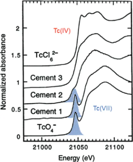
As an illustrative example, Fig. 5 shows the technetium K XANES for technetium dispersed in cement following the addition of reductants compared to the fingerprints for technetium(VII) and technetium(IV) compounds. The pre-edge associated with the technetium(VII) spectrum (shown highlighted) and the shift in edge energy are used to monitor reduction. Theoretically, calculated spectra (and other finger-printing studies) have shown this pre-peak to be indicative of photoelectron transitions to empty frontier orbitals for d-metals with tetrahedral coordination. The technetium originally in the cement samples was tetraoxidotechnetate(VII), having technetium(VII) coordinated to four oxygen atoms in tetrahedral sym-metry. The technetium K XANES spectrum for Cement 1 with no added reductant is therefore similar to the technetium(VII) reference compound, showing a strong pre-edge resonant feature. Cement 3, with added Na2S as reductant, no longer exhibits a pre-peak and has an edge energy position comparable to the spectrum for the technetium(IV) reference, allowing the interpretation that complete reduction of technetium(VII) to technetium(IV) occurred in this sample. The XANES for Cement 3 also exhibits weaker MS structures at the
Fig. 4: (a) Experimental arrangement for X-ray absorption spectroscopy (b) Cu K XAS spectrum of malachite [CuCO3.Cu(OH)2]
maximum absorption compared to that for the technetium(IV) reference, indicating that the technetium(IV) in the cement sample is less ordered structurally. A pre-edge peak in the XANES of Cement 2, containing added blast-furnace slag as reductant, remains, but its intensity is diminished. The technetium K edge is also shifted to lower energy. Both these observations indicate only partial reduction of technetium(VII) to technetium(IV) in Cement 2.
2.6 X-ray diffraction
Crystalline materials contain 3D arrays of regularly spaced atoms. X-rays are waves of electromagnetic radia-tion with wavelengths in the atomic size range: 10–10 m = 1 Å. When the X-ray waves impinge on an atom, via
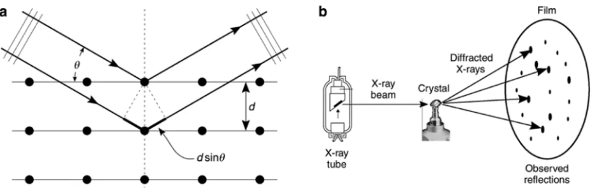
elastic or Rayleigh scattering, the cloud of electrons around each atom can scatter these incoming waves, giving rise to secondary spherical waves emanating from each scattering electron. A regular array of scatter-ers produces a regular array of spherical waves. These waves will cancel each other out in most directions through destructive interference; however, in a few specific directions that depend on the orientation of the scattering crystal’s principal axes and the spacing between the crystal’s atomic planes, constructive interfer-ence will take place. All (series of parallel) atomic planes in the crystal can be thought of as collections of scatterers constructively contributing to a diffracted beam that is formed in a direction as if reflected by that (series of) plane(s) (see Fig. 6a). Bragg reflection takes place only for those angles fulfilling Bragg’s law:
2 sin
nλ= d⋅ θ (3)
where d is the spacing between diffracting planes, n is an integer representing the diffraction order, and λ is the X-ray wavelength. Here θ corresponds to the angle that the incident beam makes with the crystal plane(s). The total scattering angle is 2θ. In cases where a single crystal is examined, this directional specificity gives rise to diffraction spots on an X-ray sensitive image detector or plate (Fig. 6b). X-rays are very suitable for pro-ducing diffraction patterns because their wavelength λ is typically of the same order of magnitude (1 to 100 Å) as the interplanar spacing in the crystal. In polycrystalline material circular Debye-Scherrer patterns are recorded instead of patterns of isolated spots. From the positions/diameters of these patterns, information on the atomic positions within the unit cell of the single crystal and on the different distances between the diffraction planes can be obtained [31].
Fig. 5: Technetium K XANES measured for cement samples containing tetraoxidotechnetate(VII) without additives (Cement 1),
added blast-furnace slag for partial reduction (Cement 2) and added Na2S for complete reduction (Cement 3), compared to
2.7 X-ray Micro Tomography
Starting with the discovery of X-rays, the penetrative character of X-rays has been exploited to produce shadow images of heterogeneous objects, including human body parts. A non-destructive inspection that is optimized to the absorption contrast in a single transmission projection image in order to distinguish the inner structure of irradiated objects is called X-ray radiography. Its 3D equivalent, X-ray tomography, makes use of an extended series of projection images recorded under many different angles between the object and the primary beam. The object rotates around an axis perpendicular to that of the source-detector while a (large) series of shadow images are recorded by means of a suitable X-ray sensitive camera (Fig. 7). Math-ematical reconstruction then allows for the creation of a virtual, 3D rendition of the object’s shape and (inner) density variations, and to visualize its inner parts without physically sectioning or otherwise destroying it. This can be done both at the macroscopic (decimeter to meter) level, e.g. in medical computed tomography, as well as at the microscopic level.
Several manufacturers offer table-top X-ray computed microtomography (XCMT) instruments with an effective spatial resolution typically situated in the 0.1 to 10 micrometre range. This type of instrumenta-tion usually makes use of cone-beams to illuminate the material under study. At synchrotron facilities, on the other hand, quasi-parallel beams are usually employed. In addition to making use of absorption contrast, where a transmission detector records the amount of radiation that is absorbed inside the irra-diated object, phase contrast can also be exploited [32]. This utilizes enhanced edge-contrast caused by interference between the original X-ray beam and its refracted equivalent. In slightly absorbing materi-als, this significantly improves the clarity with which the interfaces between various material phases may be visualized. XCMT has been successfully applied in many fields, such as engineering, chemistry, soil science, and biology.
Fig. 6: (a) Bragg reflection by a set of parallel planes with interplanar distance d. (b) Experimental setup for X-ray diffraction,
showing pattern of single crystal reflection.
2.8 X-ray sources, optics and detectors
Today, X-rays can be produced in a variety of manners suited for the generation of X-ray beams and microbe-ams, either using laboratory X-ray sources or at synchrotron radiation facilities. At synchrotrons, the dimen-sions of the primary beams used in hard X-ray microprobes are constantly shrinking. Currently (in 2018), beams of sufficient intensity with ca. 30 nm diameter can be produced using various optical technologies, while the smallest X-ray beams are on the order of 5 nm [33].
2.8.1 Laboratory sources
In the laboratory, three different types of X-ray sources can be employed: (a) sealed X-ray tubes and (b) rotat-ing anode tubes are the most commonly employed, while (c) primary X-rays produced in radioactive sources are also still utilized to a lesser extent. In most X-ray tubes, X-ray generation is realized by accelerating elec-trons to tens of kV and forcing them to decelerate rapidly when they impinge on a solid block of metal. Sealed X-ray tubes exist today in a variety of shapes and power-settings, ranging from very compact sources, e.g. those that can be integrated into portable equipment, to heavy duty, high voltage varieties suitable for the generation of X-rays up to 600 keV. Commonly employed anode materials are Cu, Mo, and W, but other high melting materials such as Cr, Rh, Pd and Ag are also popular. Some manufacturers also offer X-ray tubes with Co and Fe anodes. The power of fixed anode X-ray tubes can go up to 2 kW, while that of micro-focus sources is typically on the order of 30 to 50 W. In the latter type, the electron beam is fixed onto a small spot (typically 30-50 μm in diameter) on the anode block. The smaller the focal spot, the lower the maximum power at which the tube can be used without inflicting burn-in damage to the anode surface. In rotating anode X-ray tubes, a higher power density can be achieved by employing a rotating metal cylinder instead of the stationary anode. During each revolution, only a small part of the anode is in the electron beam, producing X-rays, while the rest can cool down [34]. An interesting new development is liquid metal jet sources, where a ribbon of molten metal (e.g. Ga, Sn) rather than a rotating cylinder of solid metal serves as anode. The liquid state of the anode allows for more efficient heat dissipation and, in combination with optimized electron optics in the X-ray tube, results in a more brilliant X-ray source [35]. Inverse Compton sources constitute another type of X-ray source situated halfway between conventional X-ray tube sources and synchrotron facilities. In these sources, X-ray generation is realized through the interaction between laser light and a highly energetic electron beam. Electron beams can be formed by impinging a high-power laser onto a pulsed gas jet and accelerating the generated plasma electrons in the laser wakefield having a high field gradient. If the accelerated electrons overlap spatially and temporally with ultrafast laser pulses in the visible range, the electrons scatter in a manner similar to an undulator insertion device at a synchrotron, but with a higher frequency (that of optical light, as opposed to undulator magnet spacing), allowing for a compact source and the possibility of table-top spectrometers [36].
2.8.2 Synchrotron X-ray sources
In a number of specialized cases, X-ray analytical methods also make use of synchrotron sources. Synchro-tron radiation (SR) is produced by high-energy (GeV) relativistic elecSynchro-trons circulating in a storage ring. This is a very large, quasi-circular vacuum chamber where strong magnets force the particles on closed trajectories. X-radiation is produced during the continuous acceleration of the particles. SR-sources are several (6 to 12) orders of magnitude brighter than X-ray tubes, have a natural collimation in the vertical plane, and are lin-early polarized in the plane of the orbit. The spectral distribution is continuous. Since the SR originates from a source point of small dimensions and is released in a very narrow angular range, it is easily focusable into micro- and/or nanobeams. An additional advantage is the high degree of polarization of SR, causing spectral backgrounds due to scatter to be greatly reduced when the XRF detector is placed at 90o to the primary beam
sources and applications are reported in Section 3. 2.8.3 X-ray microfocussing optics
The introduction and maturation of different types of (compact) X-ray optics has made the development of laboratory- and synchrotron-based hard X-ray micro and nanoprobes possible. Most, if not all, synchrotron facilities worldwide now are equipped with at least of one hard X-ray microprobe beamline, where a combi-nation of μ-XRF, μ-XAS and/or μ-XRD measurements can usually be performed simultaneously on the same material. In addition, in some cases, a combination with other methods, such as small angle X-ray scattering (SAXS) or various forms of X-ray micro/nanotomography, have been realized.
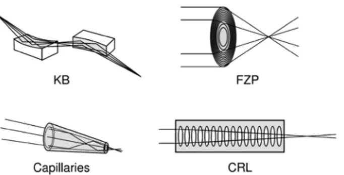
Four major types of X-ray focusing optics (Fig. 8) based on reflective or refractive focusing are currently being employed, mostly at synchrotron sources: (a) one dimensionally-curved mirrors based on total reflec-tion of the X-rays, usually in a Kirk-Patrick Baez geometry (KB optics) [37]; (b) compound refractive lenses (CRL) [38]; (c) (poly)capillary (PC) optics (also based on total external reflection) [39]; and (d) Fresnel-Zone plates (FZP), based on interference phenomena of refracted X-ray wave fronts transmitted by a patterned mask [40]. A more recent type of X-ray optics suitable for synchrotron sources are multilayer Laue lenses (MLL) [41]. Of the above-mentioned microfocussing technologies, only (poly)capillary X-ray lenses are fre-quently used in combination with laboratory X-ray instrumentation.
In recent years, the technique of confocal μ-XRF has been developed, where a secondary optic placed between the sample and detector prevents all XRF radiation, except that originating from a specific depth below the surface of the sample, from reaching the detector. This allows for an analysis of heterogeneous samples in three dimensions, with a resolution of ca. 10 to 50 μm [42–44].
2.8.4 X-ray detectors and cameras
With respect to the devices for energy-dispersive detection of X-rays, two important evolutions are worth mentioning. The first is a general move from traditional solid state (Si(Li), Ge(Li), etc.) detectors requiring permanent maintenance at liquid nitrogen temperatures towards more compact Si-PIN diodes and Silicon drift diodes (SDD) that are thermo-electrically cooled [45]. The second is the recent development of few- to multi-crystal detector arrays (e.g. Maia detector) [46] and energy-dispersive X-ray cameras [47, 48], allow-ing the detection of fluorescence radiation in a much larger solid angle than previously possible. The Maia detector, which consists of an array of 384 photodiode detectors and associated signal processing, is closely
Fig. 8: Four types of commonly employed X-ray optics: (clock wise from upper left): curved mirrors in KB geometry, Fresnel zone
coupled to a field-programmable gate array (FPGA)-based control and analysis system [46]. These develop-ments open up new methodological possibilities, e.g. for large area element-specific mapping, either via fast sample scanning or by making use of full-field detection schemes [49].
3 Synchrotron techniques and instrumentation
Synchrotron radiation is ideally suited to trace element analysis in environmental samples for several reasons, including high sensitivity and low background due to the linear polarisation. The high brilliance of synchrotron radiation enables both focussing to small beams for high spatial resolution and extremely fast acquisition rates. Hard X-ray microprobes use the deep penetration of X-rays through matter to probe and search large volumes with spatial resolution efficiently and to enable tomography. X-ray fluorescence tomog-raphy is an important method for trace element analysis in biological tissues, particularly in combination with frozen hydrated samples.
X-ray Absorption Spectroscopy (XAS), when recorded using X-ray fluorescence signal, allows for chemical speciation of dilute systems in a dense sample matrix. XAS is routinely performed on bulk samples; however, with the advent of faster scanning and acquisition schemes, XAS can also be spatially resolved. Chemical speciation of trace elements by means of XAS is a uniquely synchrotron-based technique, as it requires inci-dent X-ray energies or wavelengths that can be tuned. This is only possible for the characterisation of trace elements using monochromatic wavelengths selected from intense broad band synchrotron radiation to the required X-ray energies, which straddle the absorption edge of the element of interest. The ability to select incident excitation energy also allows unique flexibility within X-ray fluorescence microscopy. For example, it is possible to avoid signal from high concentration elements in a matrix by tuning the incident radiation below the relevant absorption edge of the high concentration element.
Ultimately, the brightness and tunability of synchrotron radiation offers versatility and fast acquisition, enabling either high sensitivity or high throughput. Sensitivity can be exceptionally high, especially for the first row transition metals. To give one example, the LD for zinc at leading edge facilities (e.g. ESRF ID16A) is 1.1 · 10–18 g (see note below).3
3.1 Relevant synchrotron-based imaging techniques
In this section, discussion is limited to those techniques capable of trace element sensitivity, with particular attention paid to those that use X-ray fluorescence contrast. Other techniques that use absorption, diffrac-tion, or scattering contrast are not always suitable for analysing trace element content, or they may have poor contrast. However, these techniques, such as X-ray absorption or phase contrast tomography, are often extremely useful for correlated studies, for example to understand the fine structural properties of a sample in which trace elements of interest occur.
Ptychography, a scanning coherent diffraction technique, is an emerging technique that can be used in parallel with scanning X-ray fluorescence microscopy and so is an ideal correlation technique. Ptychog-raphy can provide additional information about the structural environment of the trace metal(s) enriched structures.
The following synchrotron techniques will be briefly described in this section: scanning X-ray Fluores-cence Microscopy (XFM) and related higher dimensional techniques, e.g. X-ray fluoresFluores-cence tomography; XAS in fluorescence mode with spatial resolution, also as a scanning technique, alternatively described as
3 Note: In a thin carbon sample 5 μm thick, 104 zinc atoms can be detected with a 50 nm nanoprobe beam (incident flux of
109 photons per second at 10 keV, per-pixel time of 100 ms, detector solid angle of 0.2 sr), which gives 58 zinc fluorescence photons
3.1.1 X-ray Fluorescence Microscopy
X-ray Fluorescence Microscopy (XFM) is a powerful technique to quantitatively determine and map element concentrations in a wide range of sample types. Specialised microprobes at synchrotron facilities can attain spatial resolution in the tens of nm, but more typically operate within the range from 200 nm to 10 μm [50]. The extended depth of focus of X-ray probes – ranging from several hundreds of μm to mm-scale – makes these probes ideal for addressing environmental science. Analysis depth is often determined by the pen-etration of the outgoing fluorescence X-rays, and therefore depends on the X-ray energy of the interrogated element and the overall specimen matrix composition.
X-ray beam energies (e.g. 5 to 25 keV) are employed to excite core level vacancies and promote hard X-ray emission, for which the fluorescence yield is high. The beam energy can be chosen to excite the suite of ele-ments of interest, providing broad element coverage (typically from P to U), and is advantageous for detecting trace metals at sample depths beyond the reach of soft X-rays (below 3 keV). XFM typically uses an energy dispersive detector (e.g. SDD) at an angle of 90° to the incident beam to minimise scattered background. Increasing the detector solid-angle to maximize signal for a given dose increases the angular distribution of fluorescence X-rays [51], and so larger detectors have employed an annular geometry around the incoming beam (e.g. Maia detector), enabling the collection of fluorescence emission from a large solid-angle to be achieved, as well as freeing up the sample plane for both studies of large specimens and increased ranges of sample stage motion [52].
For example, XFM is capable of simultaneously mapping micronutrient elements (such as Ca, K, S), hyperaccumulated elements (such as Cd, Co, Ni, As, Se, Zn), and trace elements that are typically present in plants at far lower concentrations (such as Cu, Cr, Br) [52]. However, sensitivity is, among other things, dependent on the technical capabilities of detection systems. XFM beamlines commonly use single (or multi-element) germanium detectors (HPGe) and single (or multi-multi-element) silicon drift detectors (SDD). SDDs can handle high count rates and have excellent energy resolution (e.g. 125 eV for manganese Kα), which can be advantageous for resolving line overlaps, whereas germanium detectors are primarily used for high-energy X-rays. However, these approaches tend to be limited in their minimum time per pixel, collection solid-angle, and count-rate capacity. The Maia detector uses a large detector array to maximize the detected signal and count rates for efficient imaging. Maia enables count rates up to about 10 megacounts s−1 and uses an annular
detector geometry [53, 54]. This geometry enables a large solid-angle (1.2 steradian), while event mode data acquisition essentially eliminates readout delays. Together, these enable arbitrarily short pixel dwells (reach-ing below 100 μs). Sub-millisecond dwell times enable routine high definition imag(reach-ing (10–100 megapixels) within a single shift of experimental access [55].
3.1.2 Spatially resolved X-ray Absorption Spectroscopy
While elemental co-localization and element associations provide useful information, XAS can illuminate the element-specific molecular-scale chemical information in situ within physically intact samples of any phase [56–58]. As described in Section 2.5, XAS measures the absorption of X-rays by a sample as a function of energy across the absorption “edge” of the element of interest.
Bulk XAS has been successfully applied to reveal the overall chemical speciation of Ni and other ele-ments in plants [59–62], but local variations in speciation are difficult to detect, especially for species con-tributing to 5 to 10 % of the overall spectra. For example, Montargès-Pelletier et al. [61], found that citrate and malate were the main ligands responsible of Ni transfer within some hyperaccumulator plants by analysing different plant parts (leaves, stems and roots) via XAS. Spatially-resolved XAS approaches can determine the
variation in speciation that may occur over microns within tissues and at complex environmental interfaces, such as in the rhizosphere [63] and in oxidized pisolitic regolith [64].
XAS and XFM can be combined at suitable synchrotron facilities to provide information regarding the spatial distribution of different chemical forms of an element of interest. This is worthwhile when there is a mixture of chemical species within the sample with distinct localisations or contrasting spatial distribution, or where the size of the features of interest are comparable to the beam size [65]. In particular, XANES imaging can be employed to study samples with heterogeneous elemental concentrations and unknown chemical speciation variability. For example, Wang et al. [66] determined Se speciation in fresh roots and leaves of wheat (Triticum aestivum L.) and rice (Oryza sativa L.), showing that for plant roots exposed to selenium(VI) or selenium(IV), the majority of the Se was efficiently converted to C-Se-C compounds (i.e. methylselenocyst-eine or selenomethionine) and sequestered within the roots.
XANES maps are usually built up by “stacking” a series of XFM images, each collected with different incident X-ray energies, spanning the absorption edge of the element of interest. This is equivalent to the technique used in scanning transmission X-ray microscopy (STXM [67]). To be practical, 2D XANES mapping is contingent on the availability of extremely fast and efficient X-ray detection; otherwise, it is limited to situations where there are large spectral shifts in the XANES of species being investigated (e.g. where differ-ent oxidation states of As are presdiffer-ent). For example, localising the differdiffer-ent oxidation states of As in Pteris vittata [59] and of Se in Astragalus bisulcatus [68] has been successfully demonstrated with a limited number of energy-steps required due to the dramatic differences in energies of the different As/Se oxidation states. Recently, with ultra-fast detectors, full As K XANES spectra have been captured by registering stacks of μ-XRF maps collected at 81 energies spanning the 11.802 to 12.017 keV range in non-hyperaccumulator plants [69]. In a similar fashion, statistical analysis using principal component analysis and cluster analysis of image stacks collected in vivo across the iron K-edge allowed imaging of metal distributions and quantification of iron(II) and iron(III) content of nematodes [70]. XANES mapping also overcomes spatial drift problems that can arise when measuring XANES at a single point [65].
3.1.3 X-ray fluorescence tomography and confocal detection
The long penetration range of the characteristic X-ray fluorescence enables the acquisition of maps of the projected elemental content of thick samples. The absorption length of K-line X-ray fluorescence of light tran-sition metals is several hundred micrometers in a hydrated matrix. In order to transfer the lateral size of the X-ray probe into lateral resolution of the scanned image, appropriate depth resolution is required. A common approach is to physically section the samples. However, this procedure can be challenging and prone to artefacts. The deep penetration length of X-rays can be utilized to probe the interior of objects selectively by ‘virtual sectioning’, namely by the use of computed tomographic reconstruction methods or confocal imaging. Virtual sectioning, in combination with cryo-fixation (for biological samples) of (small) samples, can be considered minimally invasive and allows the analysis of samples with sub-micron resolution close to their native state. X-ray Fluorescence Micro-Computed Tomography (XFM-CT) enables the reconstruction of 2D or 3D elemental data from a rotation series of projection images [71, 72]. The diameter of the sample for X-ray fluorescence tomography is limited to the penetration depth of the X-ray fluorescence of the element of interest. An advantage of tomography is that the image resolution of the virtual section after tomographic reconstruction can approach the size of the probing beam.
Confocal XFM, on the other hand, allows the measurement of specific sub-volumes within a specimen. Confocal XFM does not require a rotation of the sample, but instead employs a confocal optic to confine the field of view of the energy-dispersive detector so that the signal derives from only a small portion of the illuminated column [73] (cf. Section 2.8.3). A severe limitation of confocal XFM is that the depth resolution is limited by the confocal optic to, at best, several micrometers, making 3D imaging with confocal optics less attractive at synchrotrons, where sub-micron resolution is often required. However, confocal optics of high efficiency (polycapillary optics) have been used successfully for the collection of XANES spectra from
ite, As- glutathione and As-phytochelatine complexes were identified, with varying ratios, within the leaf of the aquatic plant Ceratophyllum demersum [75]. Single voxel confocal XANES measurements are considered the most efficient way to obtain chemical speciation data at the tissue level from inside the sample without sectioning the sample or using complex extraction procedures.
3.2 Types of samples that can be analysed
X-ray techniques are extremely versatile and are uniquely placed to perform in situ studies. The basic types of samples that can be analysed range from rock to soils to biological tissues (plants and animals) and cells. Although not usually considered in the environmental science regime, metals, alloys, catalysts, and other hard materials can also be usefully studied. Hard X-rays enable measurements to be made in air, a helium atmosphere, or under a cryo-stream to maintain frozen specimens (see Fig. 9).
This enables, for example, measurements on small, or portions of large, live specimens. A specimen can be frozen in situ using a cryo-stream for samples up to about 3 × 3 mm in size.
Sample size limitations depend upon the detector geometry employed, the instrumental technique, and the sample matrix. For tomography, there is a limitation on the maximum sample diameter to ensure full penetration of the probe beam and adequate “escape” of the X-ray fluorescence, which becomes more criti-cal for lighter elements, such as P and S. Typicriti-cally, 100 μm is the maximum diameter if light elements are of interest. Additional efforts are needed to solve the self-absorption corrections required to accurately map lighter elements and correctly quantify their concentrations. For heavier elements this is less of an issue. For example, single slice tomography has been performed on a sample with diameter 1.0 mm [72] for As detec-tion. Samples that naturally have a cylindrical shape, e.g. plant roots and stems, are ideal for tomography analyses. However, most of the samples can often be cut to the required shape and size, taking care that the
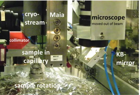
Fig. 9: Cryogenic X-ray fluorescence tomography set-up with Maia detector at the P06 Microprobe experiment (DESY, Hamburg,
Germany). A plant tissue sample inside a capton capillary mounted on a magnetic sample holder was plunge-frozen and placed on the goniometer head under an FMB Oxford cryo-stream with custom-made nozzle extension. Piezo stages for centering the capillary, the air-bearing rotation and translation stages are covered with an Al foil for protection. Courtesy P06 Falkenberg/ Küpper [72].
cut surfaces are omitted from the final analysis due to potential damage or trace element relocation and/or contamination.
X-ray analysis can be performed on exceedingly small sample volumes. For example, a 1 μm2 incident
beam illuminating a 20 to 40 μm plant sample thickness detects femtograms of the element of interest in absolute terms, which translates to 10 to 100 μg g−1 local concentration in the plant tissue [65].
Fast, efficient, on-the-fly raster scanning can avoid prolonged X-ray exposure at each position on the sample and reduce the potential for radiation damage. Nonetheless, radiation damage is still the key limita-tion of the technique, given the requirement to repeatedly scan the sample at a number of incident energies, especially for XANES images, which can take many times longer to collect than standard XFM elemental distribution maps. Radiation damage can be mitigated by analysing dehydrated samples, as water mediates the redox processes involved, or by maintaining a frozen hydrated sample at cryogenic temperatures using a variety of approaches, such as nitrogen cold streams.
3.3 General overview of instruments and facilities
For more than 30 years, X-ray beamlines have been operated at almost every synchrotron. Initial experimen-tal stations for scanning X-ray fluorescence imaging were supplemented by micro-XANES spectroscopies and micro-X-ray diffraction; different optics were used to focus into the micrometre range and below. Prominent pioneer beamlines were ESRF ID22 and NSLS X26A (KB optics), APS 2-ID-E and ESRF ID21 (FZP), and DESY beamline L (PC lenses). Over the years, advancements in synchrotron emittance and X-ray optics enhanced focussing capabilities drastically, by up to three orders of magnitude in resolution. The perfection of KB mirrors has been revolutionised by the invention of a new polishing technique (DESY P06 microprobe, P10 GINIX, ESRF ID21 ID16, MAXIV nanoMAX). Coating with Multilayers allows white beam operation and focus-sing into the 50 nm range and below with high flux (ESRF ID16). Zone plates have improved in structure, size, and especially in thickness for hard X-ray application (APS 2-ID-E, APS Bionanoprobe) [76]. MLL have matured as the instrumentation for focussing below 20 nm and are already applied in user mode at the NSLS nanoprobe (HXN).
Additionally, detector development for X-ray fluorescence and X-ray diffraction has led to improve-ments of three orders of magnitude. Whereas in the past, measureimprove-ments took seconds of dwell time per image pixel, scans are now feasible in the kHz range. The count rate capability was boosted by the intro-duction of SDD and multi-element detector arrays (e.g. Maia detector). Large detection solid angle, on-the-fly scanning mode and fast data acquisition and processing introduced the third dimension in scanning X-ray fluorescence microscopy, i.e. full 3D fluo-tomography and scanning spectro-microscopy. Pioneered at the Australian synchrotron XFM beamline [77], Maia is also operated at DESY P06 Microprobe [78], NSLS II, and CHESS. A setup from cryogenic X-ray fluorescence tomography with a Maia detector, cryo-stream (from above the sample capillary), and KB system (on the right) is shown in Fig. 9. Recent advances in digital signal processing electronics also allow scanning with millisecond dwell times with single or few-element SDD (APS 13-ID GSECARS, DLS I18).
4 Applications to environmental samples
4.1 Soil
Soil is a complex environmental matrix, heterogeneous down to the nanometre scale, where minerals, organic matter (large humic substances or smaller organic molecules), water, and air are intimately mixed, providing a suitable substrate for the growth and development of soil biota, including plants, fungi, and microorganisms.
distinction has to be made between trace elements dissolved in the soil solution (mostly in a complexed form) and those present in the organic and inorganic solid phases. The analysis of dissolved trace elements mostly implies the use of methods derived from the field of aquatic chemistry. When it comes to X-ray analyses, liquid samples are not the most suitable for sensitive trace element detection, especially when using labora-tory equipment like EDXRF and WDXRF. TXRF allows low detection limits for trace elements in liquid samples (down to ng g−1), but only after complete evaporation of the solvent [79]. In this sense, TXRF analyses could be
very useful in analysing trace elements in the soil solution, especially when only a few μl are extracted (e.g. through suction cups). For highly sensitive or speciation studies, however, synchrotron X-rays techniques are preferred. For quantification purposes, soil solutions or soil extracts (e.g. from selective extractions) can be analysed with SR XRF or TXRF. However, a more interesting application is trace element speciation by XAS. For this purpose, analysing frozen samples at very low temperatures (i.e. using liquid N2 or He) is preferable, because of the better structural information attainable and the reduced radiation damage, which could either modify the oxidation state of the element or degrade the complexing molecule [80].
When dealing with trace elements in soil solid phases, X-ray based analytical methods most often give the best results compared to other analytical techniques, especially when spatially-resolved studies are needed. The total concentration of trace elements in soils can be directly quantified on solid samples by XRF or PIXE without the need of expensive and time-consuming preparation steps including digestion after drying and fine grinding. TXRF can also be used on digested soil samples after evaporation of the liquid phase. Soil powders can be analysed by XRD or XAS (as pressed pellets) for trace elements speciation in crystalline or/and amorphous solid phases, respectively. However, laboratory XRD instrumentation does not allow the detection of pure trace elements minerals, but instead detects major minerals containing trace ele-ments in their lattice [81]. Spatially-resolved X-ray techniques are certainly among the most useful methods to study trace elements in soil, since they are able to resolve (at least partially) the great complexity of this environmental matrix. μ-XRF, SEM-EDX, and PIXE are extremely valuable laboratory tools for micro-scopic soil analyses when the concentration of the element or the spatial resolution needed are in the range of 10 to 100 μg g−1 or 5 to 10 μm, respectively. For lower concentrations or higher spatial resolutions,
synchro-tron X-ray based techniques are needed [82]. These days, environmental beamlines usually permit combined analyses with spatially resolved XRF, XRD and XAS at resolutions from a few microns down to a few nanome-tres. Such techniques have been employed to identify solid phase species of (potential) contaminants in soils, assess the remediation of contaminated soils, study the transport of contaminants, evaluate fertiliser reac-tions in soils, investigate redox-sensitive elements, elucidate rhizosphere processes, and so on [9]. However, by also combining laboratory X-ray instruments (XRD, XRF, μ-XRF and SEM-EDX) with more “traditional” fractionation methods, like sequential extractions, assessments of trace element species and mobility in soil can be achieved, as reported by Allegretta et al. [83] for As in a former gold mining site (Fig. 10).
In a recent paper, Gattullo et al. [84] used a combination of all laboratory X-ray techniques (WD and ED XRF, XRD, μ-XRF, SEM-EDX, and XCMT) to evaluate the efficacy and the mechanisms of chromium(VI) remediation in a polluted soil, using glass and aluminium from municipal solid wastes as stabilising agents.
4.2 Rocks
Trace elements are studied in rocks for numerous reasons, usually related to a desire to understand geo-logical and biogeochemical processes. Applications can range from research centered on mining for precious metals extraction to understanding major environmental and climatic changes over geological history. A number of reviews of the applications of X-ray techniques to understand trace elements in broad geological research and more specifically in rocks are available (e.g. [85]).
X-ray techniques, particularly XFM and microdiffraction, are uniquely situated to analyse trace elements in rocks alongside high concentration major elements, allowing quantitative elemental mapping on many
length scales in order to understand, for example, the nature of mineral deposits. For this purpose, petro-graphic thin sections can be suitable objects to investigate, possibly using support glasses that do not contain the element(s) of interest.
Studies of ore systems require the microanalysis of samples to collect information on mineral chemistry in order to understand physiochemical conditions during ore genesis and alteration. Such studies contribute to the debate on whether precious metals are remobilised or introduced in multiple hydrothermal events [86].
Biogeochemical studies include research into beachrock formation via microbial dissolution and re- precipitation of carbonate minerals [87]. A wider environmental study looked at the release and transport of arsenic into aquifers of Bangladesh [88] to understand the geochemistry of processes that advance release and transport of As.
Besides elemental mapping and microdiffraction, understanding the oxidation state of trace elements in rocks is very important in geological and mineralogical studies. Examples include quantitative mapping of the oxidation state of iron in mantle garnet [89] and redox preconditioning in the deep cratonic lithosphere [90].
Chemical speciation mapping, or XANES imaging, is a powerful technique that has multiple applications in geology and rock research. One of the first demonstrations of XANES imaging was the study of arsenic speciation in an oxidised pisolitic regolith [64]. The same authors [64] also imaged an Fe-Mn metamor-phosed ore sample, where arsenic(III) and arsenic(V) distribution was imaged by XANES on a thin section of 3.3 mm × 4 mm (Fig. 11). Chemical speciation mapping with XANES imaging has also been applied to many classes of environmental samples (e.g. [91]).
XFM can also be used to find very dilute and rare particles in geological systems and explore the uptake into plant systems [92]. In addition, in some cases depth resolved analyses can be done if there is sufficient detector diversity to enable analyses along various angular absorption paths [92].
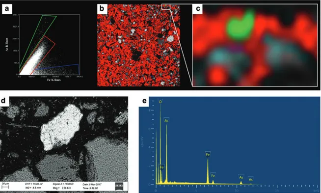
Fig. 10: μ-XRF (25 μm resolution) and FEG-SEM-EDX data of an As-polluted soil from the gold mining district of Monte Rosa
(Italy). Maps were acquired on soil thin sections (32 μm thickness). μ-XRF spectra for each pixel of the map were elaborated and the arsenic and iron K-α fluorescence peak areas were plotted (a). Three different As/Fe ratios were identified (a) and imaged with green, red and blue colors on the Si K-α fluorescence map (grayscale) of soil thin sections (b). A magnification of the μ-XRF map showing a green domain corresponding to the highest As/Fe ratio (c). (d) Backscattered SEM micrograph of the area in (c). EDX analysis of the green particle in (c) showing the presence of Fe-arsenate (most probably scorodite) (e). Modified from [83].