Deep geometry of subduction below the Andean belt of Colombia as revealed by seismic tomography

Dottorato di Ricerca in Geofisica Ciclo XXIV

Settore concorsuale di afferenza: 04/A4/Geo10: Geofisica della terra solida

Deep geometry of subduction below the Andean

belt of Colombia as revealed by seismic

tomography

Candidato Danilo Seccia

Coordinatore del Dottorato Relatore

Michele Dragoni Claudio Chiarabba

In this research project new 3D tomographic models of Colombia were calculated. I used the seismicity recorded by Red Sismica Nacional de Colombia (RSNC) during the period 2006-2009. In this time period, the improvement of the seismic network yields more stable hypocentral results with respect to older data set and allows to perform new 3D Vp and Vp/Vs models. The final dataset consists of 10813 P- and 8614 S-arrival times associated to 1405 earthquakes. Tests with synthetic data and resolution analysis indicate that the velocity model is well constrained in central, west-ern and southwestwest-ern Colombia to a depth of 160 km; the resolution is poor in the northern Colombia and close to Venezuela boundary due to a lack of seismic stations and seismicity. The 3D Vp and Vp/Vs models and the relocated seismicity indicate the existence of E-SE subducting Nazca lithosphere beneath central and southern Colombia. The changes in Wadati-Benioff zone geometries, Vp & Vp/Vs pattern, volcanism and seismicity, from North to South, show that the downgoing plate is seg-mented by slab tears roughly E-W directed, suggesting the presence of three different sectors. The seismicity volume of the northernmost sector represents most of the RNSC catalog and concentrated mostly on 100-170 km depth interval, beneath the Eastern Cordillera. In this area a massive dehydration was inferred, resulting from a delay in the eclogitization of a thickened oceanic crust in a flat-subduction geom-etry. In this sector a cluster of intermediate-depth seismicity (Bucaramanga Nest) is present beneath the elbow of the Eastern Cordillera and is interpreted as the re-sult of massive and very localized dehydration phenomenon caused by an anomalous portion of hyper-hydrous oceanic crust, like a volcanic ridge. The central and south-ern sectors, although different in Vp pattsouth-ern show, conversely, a continuous, steep

and more homogeneous Wadati-Benioff zone with overlying volcanic areas. Here a ”normal-thickened” oceanic crust is inferred, allowing for a gradual and continuous metamorphic reactions to take place with depth, enabling the fluid migration towards the mantle wedge.

Title Page . . . i

Abstract . . . iii

Table of Contents . . . v

List of Figures . . . vii

List of Tables . . . ix

Acknowledgments . . . x

Dedication . . . xi

1 Introduction and summary 1 2 Tectonic setting 7 2.1 Andean belt of NW South America . . . 7

3 Method 13 3.1 Local Earthquake Tomography . . . 13

3.1.1 Resolution . . . 17

3.1.2 Ray-tracing . . . 19

4 Seismic network and seismicity 21 4.1 Red Sismica Nacional de Colombia (RSNC) . . . 21

4.2 Seismicity of Colombia . . . 25 4.2.1 Bucaramanga Nest . . . 29 5 Velocity structure 33 5.1 LET . . . 33 5.2 Solution quality . . . 36 5.2.1 Sensitivity tests . . . 41 5.3 Results . . . 47 5.3.1 Horizontal layers . . . 50 5.3.2 Vertical cross-sections . . . 51 v

6 Discussion 56 6.1 Effect of the heterogeneity of the Nazca plate on subduction dynamics 56

6.2 Northern Andean margin . . . 58

6.3 Colombian Andes . . . 61

6.4 Intermediate depth seismicity . . . 69

6.4.1 Bucaramanga Nest . . . 71

6.5 Volcanism . . . 72

6.6 Comparison with other seismological studies in the Andean margin . 74

7 Conclusions 76

A RSNC station list 89

1.1 Regional scale tectonic of northwestern South America . . . 2

1.2 Seismicity and volcanism of northwestern South America . . . 4

2.1 Tectonic map of Colombian Andes . . . 8

4.1 Colombian seismic network in its present-day configuration. . . 23

4.2 Seismicity recorded by RSNC during the period 1993-2009. . . 24

4.3 1D used model for earthquake location and Wadati diagram. . . 25

4.4 Earthquake location statistics. . . 26

4.5 1D location of selected earthquakes. . . 28

4.6 CMT Harvard solution in Bucaramanga area . . . 31

4.7 A close look to the BN. . . 32

5.1 Tomographic invertion setup. . . 34

5.2 Trade off curve to determine damping . . . 35

5.3 DWS vs. Spread Function plot. . . 37

5.4 The 70% smearing contour for inverted nodes . . . 38

5.4 The 70% smearing contouring for inverted nodes (continued). . . 39

5.5 The 70% smearing contouring for inverted nodes - sections. . . 40

5.6 Synthetic test - horizontal layers. . . 43

5.7 Synthetic test - vertical sections. . . 44

5.8 Checkerboard test. . . 46

5.9 Tomographic results - horizontal layers. . . 48

5.9 Tomographic results - horizontal layers (continued). . . 49

5.10 Tomographic results - cross sections. . . 52

5.10 Tomographic results - cross sections (continued). . . 53

6.1 Seismicity and volcanism in Southern and Central America. . . 57

6.2 Schematic tectonic map of North West South America . . . 60

6.3 Interpretative sketch of North West South America. . . 64

6.4 Relocated seismicity - cross sections. . . 65

6.5 Break-up of the Farallon plate. . . 67 6.6 Cross section along strike of the Eastern Cordillera. . . 68

5.1 Tomographic inversion - summary . . . 36 A.1 List of RSNC permanent stations. . . 89 B.1 List of station used in the tomographic inversion. . . 91

First of all, I would like to thank my PhD advisor Claudio Chiarabba, for his sup-port throughout my studies. I’m grateful to him for introducing me in the world of scientific research and for being very open-minded. I am greatly indebted to Pasquale De Gori for the precious and friendly assistance during this years of collaborations. Thanks to Fabio Speranza and Claudio Faccenna for the constructive discussions and for providing relevant suggestions to improving the contents of this thesis. Thanks to German Prieto for the fruitful scientific collaboration in Bogot`a. A special thank goes to Viviana Dionicio, for her friendly hospitality and assistance during the months

spent in Bogot`a. Thanks to all the people at INGEOMINAS-RSNC who have been

made possible this study.

Un ringraziamento speciale va alla mia ”compagnuccia di banco” Marina, che mi ha supportato e sopportato durante questi ultimi mesi di lavoro febbrile sulla tesi. Grazie a Peppe e Betta per le pause-sigaretta al muretto e le chiacchiere in libert`a. Un ringraziamento anche a tutti i ”pollajoli” e ai colleghi-amici dei piani alti, con i quali ho condiviso momenti di scienza ma soprattutto momenti di svago, in particolare a Pamela, Michele, Mauro, Mario, Paola e Francesca. Grazie anche a Luigi, per tutte le sigarette che gli ho scroccato. Grazie a Federica per esserci stata, in un modo o nell’altro, in questi anni. Infine grazie ai miei genitori, che ancora mi sopportano dentro casa e continuano a credere in me.

Introduction and summary

The Andean belt of Colombia provides a striking opportunity to investigate the geodynamics of northwestern South America. The tectonics is complex, resulting from the interaction of three different lithospheric plates: Caribbean, Nazca and South America. The structural style, the pattern of volcanism and the distribution of earthquakes make the region an intriguing challenge in the comprehension of sub-duction dynamics.

The deformed belts are the expression of a complicated tectonic assembly under-lain by interacting oceanic slabs at depth. Previous studies have suggested relations between flat slabs, volcanism, and surface deformation in the more southerly Andes [Jordan et al., 1983; Gutscher et al., 1999; Gailler et al., 2007]. However, the tectonics of Colombia is still unclear and represents an interesting test-case for studying flat slabs vs. normal subduction. Underneath Colombia, the eastward subducting Nazca plate is inferred to be segmented by some slab tears. A smaller, southeast flat dipping slab, associated with the Caribbean plate, may be subducting, even if this feature

is under debate. Between these structures an intermediate-depth seismicity cluster (“Bucaramanga nest”) is present, and the driving force is still unclear. The leading hypothesis are a slab-slab interactions, and/or dehydration embrittlement, or local heterogeneity of the downgoing plate. The previous models are, in general, not well constrained, and the forces involved in the processes not completely clarified.

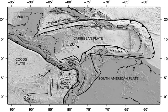
−95˚ −95˚ −90˚ −90˚ −85˚ −85˚ −80˚ −80˚ −75˚ −75˚ −70˚ −70˚ −65˚ −65˚ −60˚ −60˚ 0˚ 0˚ 5˚ 5˚ 10˚ 10˚ 15˚ 15˚ 20˚ 20˚ −95˚ −95˚ −90˚ −90˚ −85˚ −85˚ −80˚ −80˚ −75˚ −75˚ −70˚ −70˚ −65˚ −65˚ −60˚ −60˚ 0˚ 0˚ 5˚ 5˚ 10˚ 10˚ 15˚ 15˚ 20˚ 500 km 20˚

SOUTH AMERICAN PLATE COCOS PLATE CARIBBEAN PLATE CAYMANTHROU GH PANAMA CHOCO BLOCK NAZCA PLATE 71 20 54

Figure 1.1: Regional scale tectonic context of Colombian Andes and northwestern South America with crustal velocity (mm/yr relative to stable South America)

The Colombian Andes represent a remarkable chance for a new seismological study because numerous intermediate-depth earthquakes can be used for imaging, and large along-strike variations in seismicity rate provide hints on deep dynamics and surface deformations. The region represents an ideal case-study to test subduction models (e.g. continuous slab dynamics vs. delamination), the origin of intermediate depth

seismicity, and the relations between magmatism and deep dynamics. The Colombian Andes developed from the collision of two major plates, Nazca and the Caribbean, and the Panama block. This leads to complex crustal motions and surface deformation [Taboada et al., 2000; Pennington, 1981; Trenkamp et al., 2002]. According to GPS data, with respect to the fixed South American plate, the Caribbean plate moves towards the east–southeast, while the Nazca plate motion is roughly towards the east, and the northern Andes motion is towards the northeast (Figure 1.1).

This complex pattern of plate motions produces a broad zone of continental defor-mation into the Colombian and Venezuelan Andes. The defordefor-mation is accompanied by a complex pattern of the shallow seismicity, occurring on many separate faults that are distributed over several hundreds of kilometers away from the accepted plate boundaries between the South American plate and the Nazca and Caribbean plates [Corredor, 2003]. There are remarkable tectonic features which need to be included in definitive dynamic models. For many topographic and structural elements only an ambiguous geodynamic explanations is provided. Large, along-arc variations in seismicity and volcanism exist (Figure 1.2), and abundant intermediate-depth seis-micity delineates slab geometry and can be used for seismological imaging. This makes the region an excellent place to test continuous slab morphology change vs. tearing vs. break-off vs. lithospheric delamination modeling (e.g. close to tears or Bucaramanga).

The main objectives of this study are the improvement of the knowledge on the main seismogenetic structures underneath Colombia and the quality imaging of the subducting slab(s), to constrain depth, kinematics and spatial orientation of the

sub-duction system. The reconstruction of the slab geometries and interactions will help to understand the dynamics of Nazca subduction and will give new insights into plate tectonics in general. Colombia is a timely target for making major advances on these scientific issues because of the recent improvements in the political situation.

−81˚ −78˚ −75˚ −72˚ −69˚ −3˚ 0˚ 3˚ 6˚ 9˚ 12˚ 15˚ 200 km 0 40 80 120 160 200 depth[km]

Figure 1.2: Seismicity and volcanism in northwestern South America.

Earth-quakes recorded in the time period 1993-2009 are shown. Ipocentral

locations downloaded from National Earthquake Information Center website (NEIC -http://earthquake.usgs.gov/regional/neic/). Red triangles represent volcanoes.

This study has been made possible thanks to the cooperation between the Istituto Nazionale di Geofisica e Vulcanologia (INGV) and the Instituto Nacional en Geologia y Miner`ıa (INGEOMINAS), the Colombian institution which operates the National

Seismological Network of Colombia. The recent improvement of Colombian seismic network (from 2005) and the availability of new data from INGEOMINAS allow for the calculation of new velocity models enabling 3D quality imaging of subduction zones.

The thesis is organized as follows:

- Chapter 2 summarizes the relevant geological and geophysical background infor-mation from North West South America and Colombia. In order to understand seismogenesis and velocity information along the subduction zone it is necessary to define incoming and overriding plate characteristics through the subduction system.

- Chapter 3 provides the basic steps of the travel times inversion algorithms. The 3D seismic velocity structure, hypocenter locations and station corrections are calculated iteratively and simultaneously in a well constrained and worldwide adopted code, SIMULPS. The RKP ray-tracing was adopted in this study, being more robust in calculating long ray-paths with respect to the traditional ART-PB ray tracing, originally implemented in the code.

- Chapter 4 focuses on the Colombian Seismic Network and seismicity in Colom-bia. An outlook on recent development of the Red Seismological Nacional de Colombia (RSNC) is given. Special attention is paid on the presence of the Bucaramanga intermediate-depth seismic nest.

models, together with the resolution analysis and the synthetic tests.

- Chapter 6 provides interpretations on the the Vp and Vp/Vs tomographic mod-els. The results indicate a strong heterogeneity of the subducting Nazca plate, partially segmented by some tears. The differential subduction process produces the tectonic assembly of Colombian Andes and the uneven distribution of deep seismicity. The Bucaramanga Nest could be related to a local anomaly of the downgoing Nazca plate, which produces massive and localized dehydration.

- Chapter 7 summarizes the main results obtained in this study. The new to-mographic models give new insights into the structure of Colombian Andes, helping to understand the subduction dynamics.

Tectonic setting

2.1

Andean belt of NW South America

The northern termination of the Andean chain along the northwestern margin of South America (SA) is a complex belt system, spreading northward like tree branches entering Panama and Venezuela [Pindell and Barrett, 1990; Taboada et al., 2000; Cort´es et al., 2005]. The ∼ 200 km wide Andes of Ecuador expand northward to ca. 600 km, yielding the Western, Central, and Eastern Cordillera of Colombia. The Western Cordillera is in turn in tectonic contact with the Panama Arc, while at the northern margin of SA the triangular Maracaibo Block, bounded by strike-slip faults and narrow orogens, transfers deformation within Venezuela and Caribbean-SA boundary. To the south, these belts merge together and masking the original relationships and evolution. The northern termination of the Andean chain along the northwestern margin of South America (SA) is a complex belt system, spreading northward like tree branches entering Panama and Venezuela [Pindell and Barrett,

1990; Taboada et al., 2000; Cort´es et al., 2005] (Figure 2.1).

The diffuse tectonic deformation of northwestern SA arises from its complicated interaction with the Nazca and Caribbean oceanic plates and the Panama Arc.

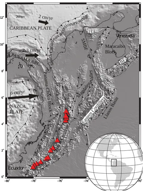
−80˚ −78˚ −76˚ −74˚ −72˚ −70˚ 0˚ 2˚ 4˚ 6˚ 8˚ 10˚ 12˚ −80˚ −78˚ −76˚ −74˚ −72˚ −70˚ 0˚ 2˚ 4˚ 6˚ 8˚ 10˚ 12˚ 200km PANA MA ARC Venezuela Ecuador Easte rnCordi llera Cent ralC ordi llera West ern Cordi llera Maracaibo Block SMB F Llanos Basi n Mag dale naV al le y Pa na m a-C hoc o B loc k NAZCA PLATE CARIBBEAN PLATE BF So ut hC ar ibbe anac cret ionary w edge 6 cm/yr 2 cm/yr 2-3 cm/yr

Figure 2.1: Shaded relief map of the North west South America. The major tectonic elements are shown. Black arrows indicate the crustal velocity relative to stable South America. Red triangles indicate volcanoes. The inset indicates the world location of the study area.

Global plate motion models [DeMets et al., 1990], along with GPS data gathered since the 1990s from SA, Panama Arc, and Pacific/Caribbean islands [Trenkamp et al., 2002] give a first-order picture of relative plate motion. The ca. 6 cm/yr E-W convergence between Nazca and SA is mainly (yet not completely) accommodated along the Nazca subduction zone, yielding 7.5 ≤ M ≤ 8.8 earthquakes during the XX century. According to Trenkamp et al. [2002], a percentage of such convergence is transferred to the Andes of Colombia and the Maracaibo Block, which are escaping towards NE at 6 mm/yr. The Caribbean Plate is moving 2 cm/yr ESE with respect to SA, and its oblique convergence seems to be partitioned into a well-developed orogenic wedge (South Caribbean accretionary wedge), and a swarm of E-W right-lateral strike-slip faults. While the formation of the Western and Central Cordillera of Colombia has been routinely referred to the complex history of both Proto-Caribbean and Nazca subduction, and Cretaceous-Tertiary [M¨uller et al., 1999; Pindell and Barrett, 1990; Taboada et al., 2000; Cort´es et al., 2005] accretion of oceanic and continental terranes to SA, the orogenic process generating the Eastern Cordillera has been a matter of long debate.

The Eastern Cordillera of Colombia

The Eastern Cordillera is an intra-continental orogen inverting a late Jurassic-Cretaceous extensional basin [Colletta et al., 1990; Dengo and Covey, 1993; Mora et al., 2006]. It is a bivergent thick-skinned chain, with main eastward tectonic trans-port towards the Llanos foreland basin, and retro-vergent (westward directed) thrust sheets stacked in sequence towards the upper Magdalena Valley [Bayona et al., 2008;

Parra et al., 2009; Mora et al., 2010]. Although conglomeratic events, angular uncon-formities, and uplift inferred from thermochronological data have been referred to late Cretaceous-Tertiary tectonic episodes [Cort´es et al., 2005; Parra et al., 2009], clear evidence for thrust-sheet emplacement onset in the Eastern Cordillera is constrained to mid Miocene times (ca. 15 Ma) during the “Andean” tectonic episode [Colletta et al., 1990; Dengo and Covey, 1993; Bayona et al., 2008]. Beneath the Eastern Cordillera, deep seismicity down to 160-170 km depth has been recorded [Taboada et al., 2000]. Seismicity is concentrated in the so-called “Bucaramanga nest” (Figure 2.1), continuously releasing small magnitude (M2.5-3.0, and no event with M larger than 6.0) earthquakes within a small mantle volume at 150-160 km depth [Zarifi et al., 2007]. Three different models have been proposed so far for the origin of the Eastern Cordillera. The first model relates the origin of the Eastern Cordillera to a low-angle SE-ward directed subduction of the Caribbean plate beneath NW SA [Taboada et al., 2000; Cort´es et al., 2005]. The existence of a low-angle Caribbean slab beneath NW SA relies upon tomographic models by VanderHilst and Mann [1994], although a seis-mic Wadati-Benioff zone associated to the postulated slab has remained elusive so far. Another model suggest that deformation in the Eastern Cordillera is transferred from the to the Nazca subduction zone, via a “mid crustal detachment” branching from the Nazca subduction to the 500 km far Eastern Cordillera [Dengo and Covey, 1993; Cooper et al., 1995]. Colletta et al. [1990] suggested that the geometry of the East-ern Cordillera was due to the intracontinental subduction of the lithospheric mantle decoupled from overlying crust. The structural grain of the Cordillera oriental, shows the following remarkable features:

- The arcuate shape of the Cordillera results from the in situ inversion and re-working of early extensional fabric with very limited translation;

- Shortening decreases moving northward and southward from the elbow; the deformation of the Cordillera virtually ceased. Balanced cross section from 6°to 5°degree give an estimate of shortening around 100 km [Colletta et al., 1990; Sarmiento, 2001], 120 km [Taboada et al., 2000] or 140 km [Dengo and Covey, 1993] who adopted an eastward vergent, thin skinned model. Sarmiento [2001] also shows that the amount of shortening decreases southward. Balanced cross section on the Sabana de Bogota, from 4°to 5°N, gives from 58 km [Mora et al., 2009] to 70 km [Cort´es et al., 2005]. To the south the eastern Cordillera deformation vanish jointing the western Cordillera. To the north it also slowly decreases in the Santander around at 8°-9°north.

- Considering the outward decreases of shortening, it is most probable that the growth of the eastern Cordillera initiate in the centre, where the deformation is maximum, and propagate northward and southward. The northern of the Cordillera is bounded by the Bucaramanga fault. It probably follow the same trend and decreasing its motion northward. Inside the Cordillera is dissected by strike slip faults running parallel to the Cordillera.

- There is limited evidence of volcanism in the Cordillera. Some small volcanic deposits have been refereed to Miocene. However, volcanism could be more diffuse than previously considered. Dolerite have been recently described near Bucaramanga [Jaramillo et al., 2005; Pardo et al., 2005] where a large

Method

Within the Earth, body wave propagation is a function of the velocity of the medium. In general there is a gradual variation of the seismic velocity with depth. However the Earth is not laterally homogeneous: crustal shortening, extensional pro-cesses and volcanoes produce structural heterogeneities and thus lateral velocity vari-ations. Seismic tomography allows to image 3D velocity model of the subsurface to account for the lateral velocity variations.

3.1

Local Earthquake Tomography

Local Earthquake Tomography (LET) was introduced for the first time by Crosson [1976] and Aki et al. [1976]. Let is a powerful technique to investigate the subsurface and has been widely and successfully applied in various tectonic contexts.

The arrival time of a seismic wave at a station is a non-linear function of the hypocentral parameters and velocity field [Kissling et al., 1994]. LET allows to resolve

the initial estimates of the model parameters (velocity and hypocenter) by perturbing them in order to minimize the misfit between predicted and observed arrival times. In general, solutions are obtained by linearization with respect to a reference 1D Earth model and starting hypocentral coordinates, and the resulting tomographic images are thus dependent on the initial reference model and starting hypocentral locations. The only knowns in the LET problem are the receiver locations and observed arrival times. The source coordinates, origin times, and velocity field are unknown parameters. Therefore, the input data for every tomographic algorithm consist of the absolute arrival times from local seismic events and station coordinates.

According to ray theory, travel time T from the source i to the receiver j is expressed as:

Tij =

Z receiver

source

uds (3.1)

where u is the slowness (1/V ) along the ray path. As described above the input data for LET are the arrival times, defined as:

tij = t0+ Tij (3.2)

where t0 is the origin time of the event. Given a set of arrival times tij recorded by

a seismic network, synthetic arrival times are calculated by equations 3.1 and 3.2 by iteratively perturbing hypocentral and velocity parameters in order to minimize the residuals between observed and predicted arrival times:

rij = tobsij − t calc

Since direct solutions of the problem are in general not possible, it can be linearized and solved iteratively, if an initial guess of the model parameters close to the true solution is available. The concept of minimum 1-D model was introduced by [Kissling, 1988] referring to the 1-D model with corresponding station corrections that lead to the smallest possible uniform location error for a large set of well-locatable events. The main purpose of a minimum 1-D model is to provide an adequate reference model for 3-D tomography, ensuring that the linearization represents a solution as close as possible close to the true model [Kissling et al., 1994]. The problem may be further complicate by several factors: (1) seismic ray paths generally are not straight and are a function of the velocity model itself, (2) the distribution of seismic sources and receivers is sparse and non-uniform, (3) the locations of the seismic sources are not well known and often trade off with the velocity model, and (4) picking and timing errors in the data are common [Shearer, 1999].

The tomographic code used in this study, SIMULPS, was developed by Thurber [1983], who introduced an iterative simultaneous inversion for 3D velocity structure and hypocenter parameters using parameters separation and an approximate ray tracer. The code has been further developed through the years [Eberhart-Phillips, 1990; Haslinger, 1998] and is one of the most widely applied. Earth structure is pa-rameterized assigning velocity values of the reference 1-D velocity model to a 3-D grid of nodes. Velocity in a certain point of the model is provided by a linear interpolation between model nodes. The inversion process is terminated when a number of specified iterations is reached, or when the variance reduction ceased to be significant, accord-ing to a f-test. The adjustments of the model are obtained by minimizaccord-ing the arrival

time residuals with a damped least square algorithm. For an array of earthquakes and receivers, the arrival time residuals equation can be written in matrix notation as:

d = G m (3.4)

where the vector d contains the arrival time residuals for all observations, the matrix G the partial derivatives for hypocentral and velocity parameters, and the vector m the model perturbations in hypocenters and velocity. To solve the equation for m, the inverse of the matrix G is computed. Usually there is no unique solution to the problem becouse there are numerous undersampled nodes and/or tradeoffs in the perturbations between different nodes Shearer [1999]. This is generally due to a non-uniform distribution of sources and receivers which produces irregular ray distribution, rendering overdetermined and underdetermined model parameters in the same problem. A damping parameter (θ) is thus introduced to avoid very small or zero eigenvalues for the underdetermined parameters, which can introduce instabilities in the solution. In a damped least square sense, the equation 3.4 is resolved by:

m = (GTG + θ2I)−1Gtd (3.5)

In order to facilitate computation of the inversion, m is split into a part containing only the velocity parameters and one containing only hypocentral parameters, but retaining the formal coupling between both [Pavlis and Booker, 1980]. Thus, us-ing parameter separation, the earthquakes are relocated separately with the updated velocity model after the inversion for model parameters. The modelling is thus an iter-ative process due to the linearization and the damping. Damping depends mainly on

model parametrization and on the average observational error (a priori data variance) [Kissling et al., 2001] and can be determined by analyzing trade-off curves between model variance and data variance for single-iteration inversions [Eberhart-Phillips, 1986]. Appropriate damping values show a significant decrease in data variance with-out a strong increase in model variance, leading to the simplest model to fit the data. SIMULPS is able to solve for Vp and Vp/Vs using P and S-P travel times, respectively. In most earthquake datasets the quantity and quality of S-wave arrival times are significantly decreased with respect to the P-wave data, this causes great variations in possible artifacts and modelling errors which are minimized by inverting for Vp/Vs instead of Vs [Evans et al., 1994].

3.1.1

Resolution

To test the reliability of the tomographic models, the analysis of the Resolution Matrix (RM) is computed. Model resolution depends on data quality, node spacing and ray coverage in the volume considered. RM [Menke, 1989] is a square matrix M , where M represent the total number of the inverted parameters:

R = (MTM + θ2)MTM (3.6)

Each row of RM contains information on the volumetric estimate of parameters. A perfectly resolved node is characterized by a compact averaging vector with elements close to 1 on the diagonal and 0 elsewhere. The sharpness of the averaging vector is quantified by means of the Spread Function (SF) as defined by Michelini and McEvilly [Michelini and McEvilly, 1991]:

Sj = log  |s_j|−1 N X k=1 skj |rj| !2 Djk   (3.7)

where skj are the elements of the resolution matrix, R, and Djk are the distances

in kilometers between pairs of nodes. Each row of the resolution matrix contains P-and S-velocity parameters. In equation 3.7, the elements of the resolution matrix are normalized such that the sum of their squares is equal to one. |sj| is the L2 norm

and can be interpreted as a weighting factor that takes into account the value of the resolution kernel for each parameter. The SF compresses each row of the resolution matrix into a single number that describes how strong and peaked the resolution is for that node [Toomey and Foulger, 1989]. The smaller the SF value, the better the resolution for the model parameter. The variation of SF is controlled by node spacing and damping. The higher the distance between two nodes the higher is the value of SF. High damping values produce high values of SF. Usually a well constrained model parameter has a SF value lower than the grid node spacing.

Thurber defines a useful measure of the sampling of nodal locations, the derivative weight sum (DWS) [Thurber and Eberhart-Phillips, 1999]. The DWS provides an average relative measure of the density of seismic rays near a given velocity node. This measure of seismic ray distribution is superior to an unweighted count of the total number of rays influenced by a model parameter, since it is sensitive to the spatial separation of a ray from the nodal location. The DWS of the n − th velocity parameter αn is defined as:

DW S(αn) = N X i X j ( Z Pij ωn(x) ds ) (3.8)

where i and j are the event and station indices, ω is the weight used in the linear interpolation and depends on coordinate position, Pij is the ray path between i and j,

and N is a normalization factor that takes into account the volume influenced by αn.

The magnitude of the DWS depends on the step size of the incremental arc length ds used in the numerical evaluation of equation 3.8. Smaller step length yield larger DWS values; therefore, DWS provides only a relative measure of ray distribution and its unit of distance are unimportant. Poorly sampled nodes are marked by relatively small values of DWS. In practice, it is useful to monitor changes in the spatial vari-ation of the DWS while testing for an optimum nodal configurvari-ation [Thurber and Eberhart-Phillips, 1999]. A good parametrization, in general, maximizes the num-ber of parametric nodes within a volume and, for a damped least squares inversion, minimizes the number of poorly sampled nodes.

3.1.2

Ray-tracing

The resolving power of ray tomography depends on the accuracy of the forward cal-culations, i.e. the determination of the propagation path and travel time through the velocity model [Haslinger and Kissling, 2001]. The code used in this study, SIMULPS 14, includes two ray tracing methods. The original is the pseudo bending ray tracer (ART-PB) [Um and Thurber, 1987], in which the initial travel times are computed for a set of arcs with different radii and laying in different planes, connecting the source and the receiver; the arc that corresponds to the smallest travel time is then chosen and perturbed by pseudo-bending, i.e. the segment endpoints are moved in the direction of the largest velocity gradient. The second ray tracer (RKP) is a full

3-D shooting and perturbation algorithm, in which they ray connecting station and source is determined by varying initial azimuth and take-off angles at the source; the variation of the initial angles is performed by using first-order perturbation theory [Virieux et al., 1991; Haslinger, 1998]. Initial shooting angles for the RKP ray tracing are obtained by ART-PB ray tracing on the first iteration; subsequent ray tracing iterations use the previously determined shooting angles as initial values [Haslinger and Kissling, 2001]. Usually, the endpoint of a ray calculated by shooting methods does not coincide with the station location; the accuracy to which the ray path coin-cides with the receiver is specified by the user, considering, for example, the station location uncertainty. Using synthetic model testing, [Haslinger and Kissling, 2001] determined that both ray tracing schemes are precise within ±10 ms in travel time for ray lengths inferior to 60 km, but for longer rays, the RKP technique yields significantly smaller errors, outperforming the ART-PB.

Becouse of the large areas considered, the poor and non-uniform station coverage and the uneven distribution of earthquakes both in horizontal direction and in depth, the RKP ray tracing was preferred to the traditional ART-PB in the Colombian case study, allowing for the calculation of longer ray paths.

Seismic network and seismicity

4.1

Red Sismica Nacional de Colombia (RSNC)

Seismic data used in this study are those recorded by the Red Sismica Nacional de Colombia (RSNC), the National Seismological Network of Colombia. The availability of data from RSNC was made possible thanks to the cooperation between INGV and INGEOMINAS, the Colombian institution which operates the seismic network.

Pulido [2003] gives a complete revision of the history and recent development of RSNC as summarized in the following. The National Seismological Network of Colombia (RSNC) was sponsored by several Colombian agencies (National Office for Prevention and Attention of Emergencies and the Colombian Telecommunications Agency) as well as the Canadian Development Agency . The RSNC started its op-eration in June 1993 and consists of 20 seismic stations countrywide connected to a central station by a satellite system. The seismometers are Teledyne Geotech S-13 vertical component with a period of 1s. The data is digitized at 16 bits and 60 sps

with a dynamic range of 136db [Nieto and Escallon, 1996]. The detection threshold of the network is M4.0 in the northern part of Colombia where the stations are sparse, M3.5 in the western part (78°W to 80°W), and M2.0 in the central part. From June 1993 to June 1999, the RSNC has recorded 15581 earthquakes, mostly located in the central part of the country [Ojeda and Havskov, 2001]. Monthly bulletins describ-ing the seismic activity countrywide are published. Simultaneously to the RSNC, in 1993 INGEOMINAS started the deployment of the National Strong Motion Network of Colombia (RNAC), which was entirely sponsored by the Colombian government. The RNAC consists of 120 strong motion digital accelerographs countrywide, includ-ing a local network at Bogot`a city consisting of 29 instruments. The instruments are KINEMETRICS ranging from 12 to 19 bits of resolution (RSNC and RNAC home-page, INGEOMINAS). The local network at Bogota has been operating since 1999 and was installed following the recommendations of a Seismic Microzonation Project of Bogota [INGEOMINAS, 1997]. The Bogota network also includes three borehole instruments located at 115 m, 126 m and 184 m of depth [Ojeda et al., 2002]. The RNAC annually publishes a Strong Motion Bulletin as well as a special issues for large earthquakes. INGEOMINAS also operates three volcanic observatories that monitor the activity of the two volcanic regions in Colombia. Besides to the RSNC and RNAC, since 1987 a seismological network in the South-West of Colombia (OSSO) is operated by Universidad del Valle, as well as a local strong motion network at Medellin city, the second largest city of Colombia, operated by EAFIT. In the period 2005-2006 a process of updating and expanding of the Seismological and Volcanological System of Colombia is started, projected to the years 2011-2012. The aim is to expand networks

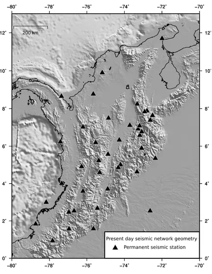
and broadband technology purchase. At present RSNC has 34 permanent stations installed, 13 broadband and 21 short period (Figure 4.1). It also has regional stations in subnets and volcanological observatories.

−80˚ −80˚ −78˚ −78˚ −76˚ −76˚ −74˚ −74˚ −72˚ −72˚ −70˚ −70˚ 0˚ 0˚ 2˚ 2˚ 4˚ 4˚ 6˚ 6˚ 8˚ 8˚ 10˚ 10˚ 12˚ 12˚ −80˚ −80˚ −78˚ −78˚ −76˚ −76˚ −74˚ −74˚ −72˚ −72˚ −70˚ −70˚ 0˚ 0˚ 2˚ 2˚ 4˚ 4˚ 6˚ 6˚ 8˚ 8˚ 10˚ 10˚ 12˚ 200 km 12˚

Present day seismic network geometry Permanent seismic station

Figure 4.1: Colombian seismic network in its present-day configuration.

Earthquake locations are routinely performed at INGEOMINAS. Phase picking and locations were accomplished using the SEISAN software package [Havskov and Ottemoller, 2005], which includes the program HYPO71 [Lee et al., 1975]. The

soft-ware was chosen because it provides a complete set of programs and a simple database structure for analyzing earthquakes, allowing phase picking with a cursor, event loca-tion, determination of spectral parameters, seismic moment, focal mechanisms, etc. A weighting scheme for quality of the P- and S-arrivals was applied. It is based on the picking uncertainty caused by noise. The weights were assigned following the HYPO71 definition. In the Figure 4.2 the seismicity recorded by RSNC during the period 1993-2009 is shown.

4.2

Seismicity of Colombia

In this study I used the entire seismic data recorded by RSNC during the years 2006-2009. In this time period, the improvement of the seismic network yields more stable hypocentral results with respect to older data set and allows to perform new 1D and 3D Vp and Vp/Vs models. A total of 20135 earthquakes were relocated using the HYPOELLIPSE code [Lahr, 1999] with the 1D model of Ojeda and Havskov [2001]. The Moho depth is fixed at 32 km depth and confirmed by the analysis of travel-time vs. distance curve (not shown here). The Vp/Vs ratio was calculated by means of the Wadati diagram (Figure 4.3). The obtained value of 1.78 is in agreement with the value calculated by Ojeda and Havskov [2001].

0 20 40 60 80 100 4 5 6 7 8 9 10 Vp(km/s) d ep th (k m) 0 2 4 6 8 10 D Ts (s) 0 2 4 6 DTp (s)

All dataset selected Vp/Vs = 1.7835 +/- 0.0004

Figure 4.3: 1D Vp model of Ojeda and Havskov [2001] used for earthquake location (left); Wadati diagram for all the analyzed events reporting the differences between P and S arrivals for each couple of station. The double differences are fitted by a linear regression. The slope of the red solid line is the Vp/Vs ratio (right).

Despite the non-uniform station coverage and the extension of the study area, the earthquakes are fairly well located in 1D preliminary location.

0 25 frequency (%) 0.0 0.2 0.4 0.6 rms (s) 0 25 frequency (%) 0 1 2 3 4 5 errh (km) 0 25 frequency (%) 0 1 2 3 4 5 errz (km) 0 25 frequency (%) 0 90 180 270 360 gap 0 25 frequency (%) −2 −1 0 1 2 res P (sec) 0 25 frequency (%) −2 −1 0 1 2 res S (sec) 0 25 frequency (%) 0 10 20 30 40 50 60 n fasi

Figure 4.4: Final location rms, horizontal and vertical errors, azimuthal gap for the locations of the whole data set, histograms of P-wave and S-wave residuals and events frequency with phases number of the whole data set.

In general, the vertical and horizontal error (Figure 4.4) are less than 5 km and the P-phase residuals are strongly peaked on the zero. The S-residuals histogram is smooth and plausibly many S phases are affected by large reading errors. This

occurrs becouse, the S phases were often picked on the vertical component of the waveform. Furthermore, the recorded signal results complicated by the long distance travelled from the source to the receiver, since the majority of the earthquakes occurr at 120-160 km depth. Most of the seismicity occurrs in the Bucaramanga Nest area. The remaining is located at the borders of mountain ranges and in the nearby of the Pacific coast.

In figure 4.5 a selection of well constrained earthquakes is shown. Hypocentral locations of events with at least 10 arrivals (P+S phases), a rms value less than 0.5 s. and a maximum azimuthal gap of 200° are plotted in map and in cross-sections. A total of 3457 earthquakes is shown.

Shallow seismicity. The seismicity defines most of the active zones of the crust along the borders of mountain ranges. The shallow seismicity across the country is associated with the N-NE trending faults within the cordilleras. To the east the seis-micity clearly delineates the Eastern Cordillera Frontal Fault along its entire length from Ecuador to Venezuela.

Deep seismicity. The selected hypocenters reveal two distinct E-SE dipping Wadati-Benioff planes beneath Colombia (Figure 4.5). Hypocenters south of 5°N clearly depict the Nazca Wadati-Benioff zone, deepening SE-ward beneath the Western and Central Cordillera. Several active volcanoes are located at 150-200 km above the Wadati-Benioff zone. Between 5°and 7°N, deep seismicity along the Nazca subduction zone almost disappears (and no volcanism occurs), while a subparallel but distinct (it is shifted inland by ca. 200 km) Wadati-Benioff plane (dipping 45°towards SE and reaching 200 km depth) appears beneath the Eastern Cordillera.

−80˚ −79˚ −78˚ −77˚ −76˚ −75˚ −74˚ −73˚ −72˚ −71˚ −70˚ 0˚ 1˚ 2˚ 3˚ 4˚ 5˚ 6˚ 7˚ 8˚ 9˚ 10˚ 11˚ 12˚ 13˚ 200 km 1 2 3 4 5 6 0 40 80 120 160 200 depth[km] 0 100 200 depth (km) −300 −200 −100 0 100 200 300 0 100 200 depth (km) −300 −200 −100 0 100 200 300 0 100 200 depth (km) −300 −200 −100 0 100 200 300 0 100 200 depth (km) −300 −200 −100 0 100 200 300 0 100 200 depth (km) −300 −200 −100 0 100 200 300 0 100 200 depth (km) −300 −200 −100 0 100 200 300 0 100 200 depth (km) −300 −200 −100 0 100 200 300 0 100 200 depth (km) −300 −200 −100 0 100 200 300 0 100 200 depth (km) −300 −200 −100 0 100 200 300 S110 section 1 N110 0 100 200 depth (km) −300 −200 −100 0 100 200 300 0 100 200 depth (km) −300 −200 −100 0 100 200 300 0 100 200 depth (km) −300 −200 −100 0 100 200 300 0 100 200 depth (km) −300 −200 −100 0 100 200 300 0 100 200 depth (km) −300 −200 −100 0 100 200 300 0 100 200 depth (km) −300 −200 −100 0 100 200 300 0 100 200 depth (km) −300 −200 −100 0 100 200 300 0 100 200 depth (km) −300 −200 −100 0 100 200 300 0 100 200 depth (km) −300 −200 −100 0 100 200 300 S110 section 2 N110 0 100 200 depth (km) −300 −200 −100 0 100 200 300 distance (km) 0 100 200 depth (km) −300 −200 −100 0 100 200 300 distance (km) 0 100 200 depth (km) −300 −200 −100 0 100 200 300 distance (km) 0 100 200 depth (km) −300 −200 −100 0 100 200 300 distance (km) 0 100 200 depth (km) −300 −200 −100 0 100 200 300 distance (km) 0 100 200 depth (km) −300 −200 −100 0 100 200 300 distance (km) 0 100 200 depth (km) −300 −200 −100 0 100 200 300 distance (km) 0 100 200 depth (km) −300 −200 −100 0 100 200 300 distance (km) 0 100 200 depth (km) −300 −200 −100 0 100 200 300 distance (km) S110 section 3 N110 0 100 200 depth (km) −300 −200 −100 0 100 200 300 0 100 200 depth (km) −300 −200 −100 0 100 200 300 0 100 200 depth (km) −300 −200 −100 0 100 200 300 0 100 200 depth (km) −300 −200 −100 0 100 200 300 0 100 200 depth (km) −300 −200 −100 0 100 200 300 0 100 200 depth (km) −300 −200 −100 0 100 200 300 0 100 200 depth (km) −300 −200 −100 0 100 200 300 0 100 200 depth (km) −300 −200 −100 0 100 200 300 0 100 200 depth (km) −300 −200 −100 0 100 200 300 S110 section 4 N110 0 100 200 depth (km) −300 −200 −100 0 100 200 300 0 100 200 depth (km) −300 −200 −100 0 100 200 300 0 100 200 depth (km) −300 −200 −100 0 100 200 300 0 100 200 depth (km) −300 −200 −100 0 100 200 300 0 100 200 depth (km) −300 −200 −100 0 100 200 300 0 100 200 depth (km) −300 −200 −100 0 100 200 300 0 100 200 depth (km) −300 −200 −100 0 100 200 300 0 100 200 depth (km) −300 −200 −100 0 100 200 300 0 100 200 depth (km) −300 −200 −100 0 100 200 300 S110 section 5 N110 0 100 200 depth (km) −300 −200 −100 0 100 200 300 distance (km) 0 100 200 depth (km) −300 −200 −100 0 100 200 300 distance (km) 0 100 200 depth (km) −300 −200 −100 0 100 200 300 distance (km) 0 100 200 depth (km) −300 −200 −100 0 100 200 300 distance (km) 0 100 200 depth (km) −300 −200 −100 0 100 200 300 distance (km) 0 100 200 depth (km) −300 −200 −100 0 100 200 300 distance (km) 0 100 200 depth (km) −300 −200 −100 0 100 200 300 distance (km) 0 100 200 depth (km) −300 −200 −100 0 100 200 300 distance (km) 0 100 200 depth (km) −300 −200 −100 0 100 200 300 distance (km) S110 section 6 N110 0 25 50 frequency (%)

Figure 4.5: Epicentral locations and depths of 3457 selected earthquakes. Hypocentral locations of 3457 events are shown. The six cross-sections in the lower portion of the plot show the projection (in a band wide of 50 km) of the hypocenters (see locations in the map). In the upper right corner of the figure a depth-frequency seismicity histogram is also reported.

The distribution of the seismicity along the strike of the Cordillera shows an abrupt shut of deep seismicity south of 5°N, a volume of seismicity descending down to 180-200 km depth from 5°to 8°N, and then a progressive shallowing of the earthquake hypocenter up to 9°N. The intense nest is located right in the centre of the Cordillera elbow. Comparison between deep seismicity and topography show that the deeper portion of the seismicity corresponds to the higher topographic relief (Figure 4.5, map). To the north the progressive shallowing of the seismicity well agree with the one of the topography. To the south, the shallowing in topography is 100 km to the south of the shut off in the seismicity, probably indicating that interaction with the Nazca slab is more evident. In this area the good fit between seismicity depth and topography indicates that regional crustal thickening, where elevation is higher, corresponds with region of deeper earthquake. Hence, earthquake distribution could be interpreted as a result of the internal dynamic of the Eastern Cordillera evolution.

4.2.1

Bucaramanga Nest

The areas of persistent and clustered seismicity are in general defined as seismic nests. In a few places in the world such seismicity occurs at indermediate-depth (70-280 km depth). The main characteristics of a seismic nest are the high activity relative to the surroundings, the concentration of hypocenters in a small volume and the continuity of seismic energy release. Within this definition, two types of nests can be distinguished: shallow nests usually related to volcanic activity and intermediate-depth nests related to subduction zones processes [Zarifi, 2007]. The shallow nests are well documented in many region of the world. For example, some nests in Japan

(Kanto district) have been suggested as shallow nests, with high rate of energy release [Usami and Watanabe, 1980]. Similar activity has been seen near volcanic areas in Central America [Stoiber and Carr, 1973], in New Zealand [Blot, 1981a], in New Hebrides [Blot, 1981b] and in the Aleutians [Engdahl and Scholz, 1977]. More than 40 such nests are identified in the circum Pacific and Indonesian arcs. This type of seismic nests can then develop by stress concentration at the margins of the weak zones of the volcanic areas [Carr, 1983].

Zarifi [2007] made a detailed and complete analysis on the known intermediate-depth seismic nests in the world. Only three intermediate-intermediate-depth nests are docu-mented in literature: the Bucaramanga nest in Colombia (hereinafter BN) at 6.8°N and 73.1°W, centered at 160 km depth [Tryggvason and Lawson Jr, 1970; Ojeda and Havskov, 2001; Frohlich et al., 1995; Schneider et al., 1987, 1972]; Vrancea in Roma-nia at 45.7°N and 26.5°E at depths between 70 and 180 km [Gusev et al., 2002]; the Hindu Kush in Afghanistan [Pegler and Das, 1998]. In deepest nest, Hindu Kush, the earthquakes tend to occur as clusters of events but the most are located at 36.5°N and 71°E in depth between 170-280 km. The focal mechanisms of earthquakes in Hindu Kush and Vrancea show reverse faulting, while in Bucaramanga the focal mechanisms are variable but the majority have reverse mechanisms (fig 4.6). Many studies agree that the seismicity in Vrancea is the result of progress of slab detachment from its upper part (slab break-off) or delamination [Koulakov et al., 2010]. The driving force in Hindu kush is yet unclear, the hypothesis are a distorted slab or a collision of two subducting slab from opposite directions.

−76˚ −74˚ −72˚ −70˚ 4˚ 6˚ 8˚ 100 km 150 155 160 165 170 175 depth[km] COLOMBIA VENEZUELA

Figure 4.6: The Harvard CMT solutions (data from 1976 to 2009) for the earthquakes in 150-175 km depth interval. in BN area.

The smallest nest is the BN (fig 4.7), representing ∼ 50 − 75% of the entire RSNC’s catalog. With respect to Vrancea and Hindu kush, the BN has the highest activity rate per unit volume [Zarifi and Havskov, 2003]. There are many studies about this nest with both local and teleseismic data, which all show that the BN has a small volume. For instance Tryggvason and Lawson Jr [1970] and Schneider et al. [1972] claimed that the BN is less than 10 km in radius. Schneider et al. [1987] found that the nest has a volume of about 8 km (NW) by 4 km (NE) by 4 km (depth) centered at 161 km depth. Pennington et al. [1979] suggested that the nest has a source volume with a diameter of 4-5 km. All of these values are based on local data. Using teleseismic data, Frohlich et al. [1995] found a volume of about 11Ö21Ö13 km3.

−80˚ −79˚ −78˚ −77˚ −76˚ −75˚ −74˚ −73˚ −72˚ −71˚ −70˚ 0˚ 1˚ 2˚ 3˚ 4˚ 5˚ 6˚ 7˚ 8˚ 9˚ 10˚ 11˚ 12˚ 13˚ 200 km BN 0 40 80 120 160 200 depth[km] 0 2 4 6 topo (km) 0 50 100 150 200 depth (km) −150 −100 −50 0 50 100 150 distance (km) S110 N110 BN section

Figure 4.7: A close look to the BN. The cross-section location is shown in the map (left).

In the BN About no events larger than M6.0 are observed, the reason is still un-known. The mechanism producing BN ”anomaly” is still unclear and under debate. Earthquakes deeper than 60 km represent 25% of global seismicity. With increas-ing depth, pressure and temperature should in theory prevent brittle failure. Many studies suggest that in BN, the driving mechanism is fluid migration or dehydra-tion processes resulting from metamorphic reacdehydra-tions [Jung et al., 2004; Hacker et al., 2003b; Preston et al., 2003]. An alternative hypothesis is a complex concentrated stress field resulting from slabs interaction.

Velocity structure

In this chapter, the tomographic inversion is described. From the relocated database, the earthquakes with the best quality, (i.e. well constrained), are selected to perform a Local Earthquake Tomography. The preferred solution is then exam-ined through resolution assessment tools and synthetic tests. Furthermore, a detailed description of the resolved velocity structure is provided. Most of the contents of this chapter are in preparation for publication.

5.1

LET

For the tomographic inversion the dataset was edited on the basis of a preliminary hypocenter location with the initial reference 1D-velocity model: I selected a subset of earthquakes with at least 6 P- and 4 S-readings, azimuthal gap less than 180°and location uncertainty less than 5 km. Applying these criteria, 1405 events recorded by 65 seismic stations were selected for the inversion resulting in 10813 P-wave and

8614 S-wave travel time observations. Assessing the appropriate model parametriza-tion is complicated by the fact that resoluparametriza-tion estimates are strongly affected by the chosen model parametrization [Kissling et al., 2001]. Coarse grid spacing yields large resolution estimates, whereas fine-grid spacing yields low resolution estimates.

200 km −80˚ −78˚ −76˚ −74˚ −72˚ −70˚ −68˚ 0˚ 2˚ 4˚ 6˚ 8˚ 10˚ 12˚ −80˚ −78˚ −76˚ −74˚ −72˚ −70˚ −68˚ 200 km

Figure 5.1: Left: Hypocentre locations (white circles), stations (black triangles), and grid nodes (gray dots) used in the inversion (left). Right: ray-coverage of the P-data set. Black triangles denote stations.

The station and earthquake distribution is highly non-uniform in Colombia (Fig-ure 5.1). There are many areas with poor station coverage and low seismicity rate, demanding a large grid node spacing. Different grid spacing were investigate and finally 50 km horizontal grid spacing was choosen. Vertical grid node spacing varies between 10 km at shallow depth (< 60 km) and 20 km at greater depth (> 60 km). Velocities of the reference 1-D model from Ojeda and Havskov [2001] (Figure 4.3) were interpolated at depth to match the gradient formulation used in SIMULPS14. This model parametrization represents the finest possible model grid spacing without

showing a strongly heterogeneous pattern of the DWS. The derivation of a minimum 1D-model Kissling [1988](not shown here) yielded no significant differences with re-spect to 1D-model of Ojeda and Havskov [2001], in terms of layering, absolute velocity value, and rms reduction. Consequently, the 1D model of Ojeda and Havskov [2001] was choosen as reference 1D model.

Damping is a critical parameter in the inversion [Kissling et al., 2001] because it affects both results and resolution estimates such as the diagonal element of the resolu-tion matrix. High damping values yields low model perturbaresolu-tions and low resoluresolu-tion, whereas low damping yield high model perturbations and good resolution. Damping depends mainly on model parametrization and on the average observational error (a priori data variance) [Kissling et al., 2001] and can be determined by analysing trade-off curves between model variance and data variance for single-iteration inversions [Eberhart-Phillips, 1986]. 0.250 0.255 0.260 0.265 0.270 0.275 data var ia nce (s 2) 0.000 0.001 0.002 0.250 0.255 0.260 0.265 0.270 0.275 0.000 0.001 0.002

model solution variance (km s-1₎2

10 50 100 200 300 500 1000 2000

Figure 5.2: Trade-off curves to determine damping parameter. The selected value is indicate by the black arrow.

Appropriate damping values show a significant decrease the in data variance with-out a strong increase in the the model variance, leading to the simplest model to fit the data. Figure 5.2 displays the trade-off curve for the tomography data set. I finally selected a damping value of 300 (see Figure 5.2) that decreased data variance significantly without strongly increasing the model variance, thus yielding a smooth solution. A damping value of 200 would also be well suited, but I preferred to select a higher and conservative damping value to avoid instabilities during the inversion.

The inversion was iterated until the variance improvement ceased to be significant, according to a f-test. The variance was reduced of 39% after 4 iterations (see Table 5.1). Inversion parameters Earthquakes 1405 P observations 10813 S observations 8614 No. of stations 65 Iteration steps 4 Damping 300 Variance Reduction 39%

Table 5.1: Tomographic inversion - summary

5.2

Solution quality

To test the reliability of the tomographic models, a complete analysis of the Reso-lution Matrix (RM) for Vp and Vp/Vs models has been performed. Each row of RM contains information on the volumetric estimate of parameters. A perfectly resolved node is characterized by a compact averaging vector with elements close to 1 on the diagonal and 0 elsewhere. The sharpness of the averaging vector is quantified by

means of the Spread Function (SF) as defined by Michelini and McEvilly [1991]. The SF compresses each row of the resolution matrix into a single number that describes how strong and peaked the resolution is for that node [Toomey and Foulger, 1989]. The smaller the SF value, the better the resolution for the model parameter. From the analysis of DWS vs spread function [Toomey and Foulger, 1989] (Figure 5.3) I choosed 3 as cutoff value of SF for both Vp and Vp/Vs models. The solution quality is further verified by sensitivity and resolution tests using checkerboard and synthetic models for Vp. 0 2500 5000 7500 dws 0 1 2 3 4 5 6 7 8 9 10 spread function - Vp 0 2500 5000 7500 dws 0 1 2 3 4 5 6 7 8 9 10 spread function - Vp/Vs

Figure 5.3: A plot of the DWS versus the spread function of the averaging vector of the model parameters for Vp and Vp/Vs models. The dashed line at SF=3.0 is the upper limit of values of the spread function values considered to be acceptable (see text for explanation).

Because the SF is computed by summing the contribution of all nodes, it gives no information on the directional properties of the parameter estimation (smearing). To analyze the smearing directions we contoured, for each node, the volume where the resolution is 70% of the diagonal element [Reyners et al., 1999].

Y= -500 Y= -400 Y= -300 Y= -200 Y= -100 Y= 0 Y= 100 Y= 200 282˚ 285˚ 288˚ 200 km 10 km 3˚ 6˚ 9˚ 200 km 20 km 200 km 30 km 200 km 40 km 200 km 50 km 200 km 60 km 282˚ 285˚ 288˚ 3˚ 6˚ 9˚ 3˚ 6˚ 9˚ 282˚ 285˚ 288˚ 282˚ 285˚ 288˚ 3˚ 6˚ 9˚ 3˚ 6˚ 9˚ 3˚ 6˚ 9˚

Figure 5.4: The 70% smearing contour for inverted nodes (crosses) with SF lower or equal to 3.0 in layers from 10 to 180 km depth for Vp model. The nodes with SF < 1.5 and 1.5 < SF < 3.0 have black and gray crosses and contours, respectively. The black dots indicated the nodes not inverted or the inverted nodes with SF > 3.0 . The arrows on the top left panel on the right border indicate the eight W-E sections shown in Figure 5.5. The Y values are the offset distances of the sections from the center of the model. (Continued on the next page)

3˚ 6˚ 9˚ 200 km 80 km 3˚ 6˚ 9˚ 200 km 100 km 200 km 120 km 200 km 140 km 200 km 160 km 200 km 180 km 3˚ 6˚ 9˚ 282˚ 285˚ 288˚ 3˚ 6˚ 9˚ 3˚ 6˚ 9˚ 3˚ 6˚ 9˚ 282˚ 285˚ 288˚ 282˚ 285˚ 288˚ 282˚ 285˚ 288˚

0 100 200 Depth (km) -500 -250 0 250 500 W _{Y = -500} E 0 100 200 -500 -250 0 250 500 W _{Y = -400} E 0 100 200 Depth (km) -500 -250 0 250 500 W _{Y = -300} E 0 100 200 -500 -250 0 250 500 W _{Y = -200} E 0 100 200 Depth (km) -500 -250 0 250 500 W _{Y = -100} E 0 100 200 -500 -250 0 250 500 W _{Y = 0} E 0 100 200 Depth (km) -500 -250 0 250 500 Distance (km) W _{Y = 100} E 0 100 200 -500 -250 0 250 500 Distance (km) W _{Y = 200} E

Figure 5.5: Same as Figure 5.4 but for eight vertical, W-E trending sections. Sections locations are shown in Figure 5.4, top left panel.

Figures 5.4 and 5.5 show the 70% smearing contour for nodes with SF < 3 in 12 inverted layers and in eight W-E trending vertical sections of Vp model. Well resolved nodes are characterized by low values of SF and smearing effects localized in the

surrounding nodes. I found that model parameters with SF< 3 have good resolution, with only slight smearing of anomalies over adjacent nodes. The resolution within the study area is fairly good beneath the Eastern Cordillera and in the western Colombia, nearby the Pacific coast at crustal depth. Deeper layers show well resolved nodes (SF values < 3) in the western Colombia, Eastern Cordillera and around the BN area. At 160 km depth the resolution is poor for most of the model. The only resolved area is in the nearby of BN. At 180 km depth, becouse of the substantial absence of seismicity, the resolution is insufficient and no resolved node is observed. In the vertical cross-sections (Y=0 and Y=100) a localized smearing effect is observed in the volume directly beneath BN, plausibly due to unidirectional ray-paths travelling westward from BN to the surface. In the northern part of the model (Y=200) few resolved nodes are observed, due to the poor station coverage. In summary, the resolution results good in the central and western-southwestern portion of the model. Northward from BN, and close to the Venezuela boundary, the resolution is poor.

5.2.1

Sensitivity tests

The solution quality was verified by sensitivity and resolution tests. The effect of the model grid spacing, dimensioning and distribution of the data on the imaging of structures can be tested with synthetic data. They can be designed on a priori geometries or on actual results: in both cases the aim is to check which parts and how many of the imposed anomalies can be restored given a 3-D grid and a station distri-bution. Another very common analysis consists of the checkerboard resolution test. In the checkerboard test, positive and negative anomalies are alternated in latitude

and longitude, and in depth. This simple alternation of positive and negative values becomes an image which is straightforward and easy to remember. Therefore, from the simple visual analysis of results and the comparison with the original distribution it is easy to understand where the resolution is poor and where it is good. The results of the checkerboard test give insights not only into which part of the model can be solved but also into the minimum and maximum size of the anomaly that can be resolved.

Synthetic test

Synthetic test were calculated using synthetic 3-D velocity models that mimics expected or a priori known real structures [Kissling et al., 2001]. The aim of the this test was to check how well the amplitudes of realistic velocity anomalies would be reproduced for a synthetic velocity model showing a similar subsurface structure as expected for the Colombia subduction zone (Figure 5.6, left column). A synthetic Vp model composed of both low and high Vp anomalies was created. I simulate a negative Vp anomaly (Vp = -10%) between 60 and 100 km depth located nearby the Pacific coast at 4°N - 5°N, and a positive Vp anomaly (Vp = +10%) elongated NE-SW and SW-dipping from 80 to 140 km, parallel to the strike of the Eastern Cordillera. Synthetic arrival times are generated, random noise added, and data are inverted using the same parameters as the real inversion. The negative anomaly is well recovered in all the layers except for the 60-80 km depth interval, where a smearing effect is observed and the recovered anomaly branches in various directions (Figure 5.6, right column).

200 km 200 km 60 km 200 km 60 km −78˚ −76˚ −74˚ −72˚ −70˚ 2˚ 4˚ 6˚ 8˚ 10˚ −78˚ −76˚ −74˚ −72˚ −70˚ 2˚ 4˚ 6˚ 8˚ 10˚ −10 −5 0 5 10 Vp(km/s) 100 km 2˚ 4˚ 6˚ 8˚ 10˚ _{200 km} 120 km 2˚ 4˚ 6˚ 8˚ 10˚ _{200 km} 140 km 2˚ 4˚ 6˚ 8˚ 10˚ 2˚ 4˚ 6˚ 8˚ 10˚ _{200 km} 80 km 200 km 100 km 2˚ 4˚ 6˚ 8˚ 10˚ 200 km 120 km 2˚ 4˚ 6˚ 8˚ 10˚ 200 km 140 km 2˚ 4˚ 6˚ 8˚ 10˚ 2˚ 4˚ 6˚ 8˚ 10˚ 200 km 80 km

st

ar

ti

n

g

rec

_over

ed

Figure 5.6: Assessment of solution quality by test with synthetic data. Left: synthetic input Vp model; right: recovered model after inversion. P-wave perturbations relative to 1-D initial reference model are shown. Horizontal layers are shown for different indicated depth. Black line outlines the best resolved region.

0 2 4 6 to po (k m ) 0 50 100 150 200 −300 −250 −200 −150 −100 −50 0 50 100 150 200 250 300 S110 N110 se ctio n 1 0 2 4 6 to po (k m ) 0 50 100 150 200 −300 −250 −200 −150 −100 −50 0 50 100 150 200 250 300 S110 N110 se ctio n 2 0 2 4 6 0 50 100 150 200 de pt h (km) −300 −250 −200 −150 −100 −50 0 50 100 150 200 250 300 S110 N110 0 2 4 6 0 50 100 150 200 de pt h (km) −300 −250 −200 −150 −100 −50 0 50 100 150 200 250 300 S110 N110 −80˚ −78˚ −76˚ −74˚ −72˚ −70˚ −68˚ 0˚ 2˚ 4˚ 6˚ 8˚ 10˚ 12˚ 200 km section 1 section 2

starting

recovered

Figure 5.7: Same as Figure 5.6 for two vertical cross sections. The top panel indicates the traces of cross-sections. Black line outlines the best resolved region.

Furthermore, at this depth, the inversion produces slight artifacts of weak positive anomalies bounding the low-Vp. The recovered high-Vp anomaly in the 80 km depth layer shows a slight offset and mislocation with respect to the original position, while, in the remaining layers, the anomaly is fairly well reproduced. In the cross section shown in Figure 5.7, both the high-Vp and low-Vp anomalies are reproduced with good approximation.

Slight artifacts of bounding opposite anomalies are observed at 60-80 km depth around low-Vp, as previously described. Figures 5.6 and 5.7 show that the inversion procedure led us to recover an average of 60-70% amplitude of the starting model.

Checkerboard test

In the checkerboard test, I used positive and negative Vp anomalies of 5% al-ternated every two nodes in latitude and longitude, and every two layers in depth. Synthetic travel times were generated and inverted, after the addition of a gaussian noise with standard deviation equal to the final variance of the inversion, using a laterally homogeneous velocity model.

The results of the checkerboard test are shown in Figure 5.8. In the crustal layers (10-30 km depth), the inversion cannot reproduce the geometry and the amplitudes of the starting checkerboard anomalies. The geometry and arrangement of the recovered anomalies are quite different form the starting model except for the central area of the model. From 40 km depth, the recovered anomalies are fairly well reproduced in the central and western-southwestern Colombia. Despite the poor station coverage and the uneven distribution of seismicity, the recovering power of the tomographic

inversion is quite good between 50 km and 100 km depth. In this depth interval the checkerboard anomalies are reproduced with good fidelity both in shape and in amplitude. At 120 km depth the resolution is still good in the central Colombia, in the surrounding area of BN and partially, nearby the Pacific coast between 3°and 5°N. At 140-160 km depth recovered anomalies are observed only in the central area of the model. 200 km 30 km 200 km 60 km 200 km 80 km −5 0 5 Vp(km/s) 2˚ 4˚ 6˚ 8˚ 10˚ 2˚ 4˚ 6˚ 8˚ 10˚ 2˚ 4˚ 6˚ 8˚ 10˚ 2˚ 4˚ 6˚ 8˚ 10˚ 2˚ 4˚ 6˚ 8˚ 10˚ 2˚ 4˚ 6˚ 8˚ 10˚ 2˚ 4˚ 6˚ 8˚ 10˚ 200 km 160 km 200 km 100 km 200 km 120 km 200 km 140 km −78˚ −76˚ −74˚ −72˚ −70˚ 2˚ 4˚ 6˚ 8˚ 10˚ _{200 km} −78˚ −76˚ −74˚ −72˚ −70˚ start

Figure 5.8: Checkerboard test. In the top left panel the Vp synthetic starting model is reported; in the remaining panels the models restored by the tomography for some layers at different depth are displayed. The black line outlined the best resolve region of the model (SF< 3).

5.3

Results

The tomographic results are presented in the form of horizontal layers (Figure 5.9) and vertical cross-sections (Figure 5.10). The figures show P-wave and Vp/Vs ratio perturbation relative to the 1D reference model. Velocity perturbation were preferred to the absolute values, being easier to interpretate. Hypocentral locations are shown for each horizontal layer within 10 km perpendicular to profile. In the vertical sections hypocentres are projected into the sections within 50 km perpendicolar to profile. The tomographic models reflect the complexity of the subduction dynamics beneath Colombian Andes. The tomographic images (in particular the horizontal layers) often show complicated Vp and Vp/Vs patterns, making the interpretation quite difficult. To avoid misinterpretations I focused my description only on the more relevants and well constrained features. Given the large reading errors affecting the S-picks (see Chapter 4), I used the Vp/Vs model only to facilitate the interpretation of the more robust Vp model.

−78˚ −76˚ −74˚ −72˚ −70˚ 2˚ 4˚ 6˚ 8˚ 10˚ _{200 km} 30 km 2˚ 4˚ 6˚ 8˚ 10˚ _{200 km} 50 km 2˚ 4˚ 6˚ 8˚ 10˚ _{200 km} 60 km 2˚ 4˚ 6˚ 8˚ 10˚ _{200 km} 80 km 200 km 30 km −78˚ −76˚ −74˚ −72˚ −70˚ 2˚ 4˚ 6˚ 8˚ 10˚ 2˚ 4˚ 6˚ 8˚ 10˚ 200 km 50 km 2˚ 4˚ 6˚ 8˚ 10˚ 200 km 60 km 2˚ 4˚ 6˚ 8˚ 10˚ 200 km 80 km −8 −4 0 4 8 −3 −2 −1 0 1 2 3 dVp/Vs(%) dVp(%)

Figure 5.9: Velocity perturbation relative to initial 1-D model in a selection of the inverted layers of the tomographic model. The black line outlines the limits of the resolved region where the SF 3.0 In each layer, I plotted the relocated seismicity occurring 10 km above and below the layer. (Continued on the next page)

−78˚ −76˚ −74˚ −72˚ −70˚ 2˚ 4˚ 6˚ 8˚ 10˚ _{200 km} 100 km 2˚ 4˚ 6˚ 8˚ 10˚ _{200 km} 120 km 2˚ 4˚ 6˚ 8˚ 10˚ _{200 km} 140 km 2˚ 4˚ 6˚ 8˚ 10˚ _{200 km} 160 km −8 −4 0 4 8 200 km 100 km 2˚ 4˚ 6˚ 8˚ 10˚ 200 km 120 km 2˚ 4˚ 6˚ 8˚ 10˚ 200 km 140 km 2˚ 4˚ 6˚ 8˚ 10˚ 200 km 160 km −78˚ −76˚ −74˚ −72˚ −70˚ 2˚ 4˚ 6˚ 8˚ 10˚ −3 −2 −1 0 1 2 3 dVp/Vs(%) dVp(%)

5.3.1

Horizontal layers

- Crustal layers. At crustal depths Vp and Vp/Vs models show complicated patterns, plausibly resulting from the structural complexity of the Andean belt. In these horizontal layers it is difficult to distinguish relevant tectonic features. Here I show only the 30 km depth layer. The main features are the presence of a localized low-Vp anomaly (Vp -5%) nearby the Pacific coast around 4°N, where a cluster of shallow seismicity is observed. Such feature can also be found in the deeper layers, to a depth of 100 km. The Vp/Vs model shows a bipartition: beneath the Eastern Cordillera a diffuse low Vp/Vs is observed; South of 5°N the model shows high Vp/Vs ratio along strike of the Cordilleras.

- 50-80 km depth layers. Within this depth interval the more relevant features are represented by the low-Vp zone (Vp -4%) which is mostly concentrated in the area nearby the Pacific coast with increasing depth, at around 4°N. Here is located part of the seismicity occurring in the Pacific coast area. The Vp/Vs ratio show, in general, diffuse high values beneath the Eastern Cordillera and, more localized, in correspondence of the low-Vp zone.

- 100-140 depth layers. In this depth range the tomographic models become more distinguishables and can be divided in two zones. (1) The Bucaramanga area is mostly dominated by high-Vp and high Vp/Vs anomalies. Narrow low-Vp zones, elongated along strike of the Eastern Cordillera, can be observed. Here the relocated seismicity is located in both positive and negative Vp anomalies. (2) Nearby the Pacific coast, between 5°and 3°N, a diffuse low-Vp anomaly can