Quantitative evaluation of household nutrition patterns: an econometric assessment of the UK 5-a-day impact on fruit and vegetable consumption

DOTTORATO DI RICERCA IN

ECONOMIA E STATISTICA AGROALIMENTARE

Ciclo XXII

Settore scientifico-disciplinare di afferenza: SECS-P/02 Politica Economica

TITOLO TESI

Quantitative evaluation of household nutrition patterns: an

econometric assessment of the UK 5-a-day impact on fruit and

vegetable consumption

Presentata da: Sara Capacci

Coordinatore Dottorato

Relatore

Prof. Roberto Fanfani

Dott. Mario Mazzocchi

The present thesis would not have been possible without the outstanding supervision I have been receiving from Dott. Mario Mazzocchi. The work also benefitted a lot from the time I spent at the Department of Agricultural and Food Economics at the University of Reading, UK. Thanks are also due to the colleagues and friends of the coloured and funny working environment of Via Zamboni 18.

CONTENTS

1. Introduction ... 4

1.1 Effectiveness of the 5-a-day interventions in western countries... 6

2. Methodology ... 8

2.1 Evaluation ... 8

2.2 Estimation of counterfactual demand through a demand model... 10

2.3 Information and demand function ... 13

2.4 The Almost Ideal Demand System (AIDS) specification and its linear version (LA/AIDS). ... 14

2.4.1 AIDS and LA/AIDS elasticities ... 16

2.5 Differences in demand responsiveness to income changes: the Quadratic Almost Ideal Demand System (QUAIDS)... 16

2.6 Heterogeneous preferences: demographics in the AIDS model... 18

2.7 Demographic effects in the Quadratic Almost Ideal Demand System... 20

2.8 Price and expenditure endogeneity ... 22

2.9 Estimation of the campaign impact through the counterfactual demand. ... 23

3. Application ... 25

3.1 5-a-day campaign in the UK ... 25

3.2 Previous evaluations of the 5-a-day campaign... 25

3.3 Data: Expenditure and Food Survey ... 26

3.4 Some descriptive statistics: average fruit and vegetable consumption ... 27

3.5 Pre-post comparison of consumption levels... 34

3.6 Model specification. ... 35

3.6.1 Unit values and quality effects. ... 35

3.6.2 The demand system... 37

3.7 Empirical results... 39

3.7.1 Elasticity estimates... 43

3.7.2 Selection of the model... 44

3.7.2.1 Model comparison criteria: nested and non-nested models ... 44

3.7.2.2 Alternative specifications and selection of the model... 46

4. Conclusions ... 52 Appendix...55 Reference List...70

LIST OF TABLES

Table 2.1 Compensated and uncompensated elasticities. ... 13 Table 2.2 Elasticity formulas in LA/AIDS and AIDS models... 16 Table 2.3 Uncompensated price elasticities in AIDS, LA/AIDS, AIDS with demographic effects, QUAIDS and QUAIDS with demographic effects... 21 Table 2.4 Uncompensated income elasticities in AIDS, LA/AIDS, AIDS with demographic effects, QUAIDS and QUAIDS with demographic effects... 22 Table 3.1 Average per capita fruit and vegetable purchases by income quartile (grams per week). ... 29 Table 3.2 Average number of F&V portions per day by income quartile (per-capita)... 30 Table 3.3 Average per capita fruit and vegetable purchases (grams per week), DEFRA computation strategy. ... 31 Table 3.4 Fruit and vegetable unit values by income quartile (pound per kilogramme) and retail price changes... 32 Table 3.5 Change in per capita fruit and vegetable consumption with respect to baseline period (2002-03) by income quartile... 35 Table 3.6 Demand system regression results (years 2002-03, 2003-04, 2004-05, 2005-06)... 41 Table 3.7 Test of symmetry and homogeneity constraints for 2002-03 demand system... 42 Table 3.8 Wald tests for quadratic specification and demographic effects (for all years)... 43 Table 3.9 Direct and cross price elasticities and food expenditure elasticities (years 2002-03, 2003-04, 2004-05, 2005-06)... 43 Table 3.10 Description of five alternative model specifications... 47 Table 3.11 Model comparison... 48 Table 3.12 Impact of the 5-a-day campaign on fruit and vegetable consumption (quantity of fruit and vegetables consumed per person per week). ... 49 Table 3.13 Impact of the 5-a-day campaign on aggregated fruit & vegetables consumption (quantity of fruit and vegetables consumed per person per week)... 51 Table 4.1 Model-estimated impact of the 5-a-day campaign and pre-post consumption comparison. ... 53

1. Introduction

Healthy food habits have been shown to be the first prevention tool against most of non-communicable chronic diseases, including heart diseases, stroke and cancer (WHO, 2003). Adequate consumption of fruit and vegetables (F&V) represents a crucial element of healthy eating. Unfortunately, actual intakes are still largely below the recommended level of 5 portions of F&V per day (about 400 grams per person per day) almost everywhere in western countries (Naska et al., 2000).

During the last ten years, the World Health Organization has explicitly asked countries to set out effective health communication programmes to improve people dietary choices, in order to reduce the risk of deaths from chronic disease.

The question of unhealthy diets has become a new policy priority for the government of most western countries, and the debate about which intervention might affect effectively people food habits is much-discussed.

The “5-a-day” campaign to increase fruit and vegetable intakes towards the WHO recommendation of 5 portions (or 400 grams) per day was first introduced in 1991 in the US and subsequently it has been adopted by several other countries (Stables et al., 2002). Today it represents one of the most widespread public interventions in the field of healthy eating. In the UK it has started as a nationwide communication campaign in 2003.

The demand for unambiguous evaluations of public interventions effectiveness and the need for detecting the proper policy instruments in the nutrition field has increasingly involved economists, as it has already happened for other public policy debates (e.g. environment) (Mazzocchi et al., 2009).

Under the economic perspective consumers make their decisions on purchases (including food purchases) based on their preferences, market price levels for different goods and disposable income. Economically optimal decision requires that consumer hold full information when making their choices, including knowledge on the health implications of alternative consumption bundles.

Since the full information assumption may not be reflected in the market, one of the main objectives of public intervention is to fill information gaps. In economic terms, the absence of perfect information leads to market failure. People may develop unhealthy food habits unwillingly, because they do not have adequate information about the health consequences of their food choices. Either they do not have adequate information about the nutrient contents of

different food items, or about the proper portions to be consumed in a day. This lack of information might create a discrepancy between rational and welfare optimising choices for consumers. For instance, people can gain utility from intangibles like health, but might fail to maximize their utility because asymmetric or incomplete information on nutrient food content prevents them to achieve the desired nutrient intake levels. According to mainstream economics, governments must intervene to address market failures and restore the adequate environment for free market choices.

Yet, this is not the sole possible scenario. Perfectly informed individuals may have different preference structures and attach different importance to pleasure and health. Thus, well-informed people might consciously choose to have an unhealthy diet, preferring short-term gratification with regard to possible long-term health risks (Mazzocchi et al., 2009).1

Moreover, even in a perfectly informed market, people wishing to maximize their demand of health through food choices can be hindered by their budget constraint, or by price levels of the healthier food.

Public intervention aimed at taking part in this mechanism should be planned considering all the acting forces. In fact even if information is a precondition of good diet, policies addressing information problems are not necessarily the most effective ones for improving diets. Adopting a pure public health perspective leads evaluators and policy makers to ignore possible interaction with those market forces which normally are considered in the economic field.

This thesis adopts an empirical economics perspective, with the aim of providing an ex-post quantitative evaluation of the UK 5-a-day programme impact on fruit and vegetable consumption of British households. Microeconomic models as demand systems are employed here to stylize consumption behaviour which results from alternative acting forces, and the estimate of the counterfactual scenario (without the policy) is based on econometric methods which are expected to disentangle the policy impact from potentially conflicting market forces dynamics.

We estimate a demand model for fruit and vegetables based on the Quadratic Almost Ideal Demand System (QUAIDS), allowing for demographic effects, and controlling for potential endogeneity of prices and total food expenditure. The model, estimated for the baseline period (prior to the intervention), is then projected to estimate the counterfactual demand for fruit and vegetables over the years following the information campaign for which data are available. The coefficients of the demand model which are estimated on pre-campaign data represent the reference behavioural parameters for assessing consumer response to the campaign over the following years. The difference between the post campaign consumption

1 _{Researchers have shown that when risks are well known public information campaigns are ineffective in changing}

behaviours (Rindfleisch et al., 1999). In other words when perfect information is granted market forces act to determine consumers’ choices.

(forecasted through post-campaign estimated model) and the model-projected consumption is an estimate of demand response to the campaign, after controlling for price and expenditure variations over the years.

The work is organized as follows: the next section offers a brief description of the 5-a-day programmes implemented and evaluated by western countries in the last 15 years. Chapter 2 presents the theoretical tools employed for counterfactual estimation and ex-post evaluation with a particular focus on the demand system specification. In Chapter 3 the application to the UK case is described. Finally results are summarized and conclusions drawn.

1.1 Effectiveness of the 5-a-day interventions in western countries.

Five-a-day campaigns are currently in action in the US (“5-a-day for better health” promoted by the National Cancer Institute), in Western Australia (“Go for 2&5 campaign”), in Spain (“5 al dia” programme), in Portugal (“Programa 5 ao dia”), in Denmark (“6-a-day”), in Poland, in Sweden (driven by the Swedish supermarket chain) and in the UK2.

Because of the employed communication tools and strategies, 5-a-days programmes can be defined as social marketing interventions. According to Andreasen’s definition

Social marketing is the application of commercial marketing technologies to the analysis, planning, execution and evaluation of programs designed to influence the voluntary behaviour of target audiences in order to improve their personal welfare and that of society (Andreasen, 1995).

The literature above effectiveness of social marketing interventions in nutrition field is quite rich. The balance of evidence is that normally interventions are effective in raising awareness, increasing knowledge and self-efficacy, and changing attitudes, but they are less effective in changing behaviours (Mazzocchi et al., 2009).

A detailed literature review of ex-post impact assessment studies for policies promoting fruit and vegetable consumption in Europe and US has shown that the average effect on consumption is roughly between +0.2 and +0.6 portion per day (Pomerleau et al., 2005). Western Australian Go for 2&5 evaluation has been based on a pre-post survey and has highlighted an increasing of 0.8 servings/day for adults during the program period, with a following decrease of 0.3 portions after the end of the campaign (Pollard et al., 2008).

2_{This information has been collected within the project “Interventions to Promote Healthy Eating Habits:}

Evaluation and Recommendations – EATWELL” funded by the European Commission (7th _Framework

In the US, the impact assessment of the worksite-based interventions included in the 5 a day for Better Health campaign has shown a pre-post increasing of 19% of consumption levels, reflecting a difference of one half serving (Sorensen et al., 1992)

The evaluation of the whole US 5 a day program (which is made up of multiple initiatives, designed at national level and locally implemented) through two nationally representative pre and post surveys (in 1991 and in 1997) has shown a statistically significant improvement in consumption level from baseline to follow-up survey (from 3.75 to 3.98 per day for the total population). However the adjusted analysis revealed that the positive change was probably attributable to demographic changes between the two survey years, correlated with vegetable and fruit consumption. Nonetheless the same study points out that the program awareness (measured as the percentage of people aware of the 5 a day message) has significantly changed among the total population and all the demographic subgroups (Stables et al., 2002). The next chapter will focus on the evaluation strategy employed for impact assessment of the UK 5-a-day.

2. Methodology

2.1 Evaluation

The objective of the present work is an ex-post evaluation of the effect of the 5-a-day intervention on UK consumers. Some preliminary definitions are needed.

With reference to the policy evaluation literature, the 5-a-day campaign here considered is what is called the treatment, i.e. a policy, or intervention explicitly directed to a group of units (individuals, firms, etc.) and explicitly pursuing a change in some dimension of that group. The group of units to which the treatment is directed is the target group.

Some variables can be found to effectively describe those dimensions of the target group the treatment should affect (e.g. psychological traits, behaviours, etc.); they can be defined as

outcome variables, or outcomes. The 5-a-day campaign is meant to affect at least two

dimensions of its target group (UK consumers): attitudes (i.e. mostly knowledge and awareness of the importance of eating more fruit and vegetable) and behaviour (i.e. actual consumption) and ultimately they are expected to have a positive effect on health and life expectancy. The aim of the present work is to assess the effect of the campaign on behaviour. Thus, fruit and vegetable consumption is the evaluated outcome.

The effect or the impact of the intervention is often erroneously confounded with the simple difference between the outcome level observed before the treatment on the target units and the outcome level observed after the treatment on the same units. This difference ignores the possible outcome’s own dynamic due to many factors other than the intervention. Consumption patterns normally evolve over time, even in absence of specific public policies. As it will be discussed later, consumption can be strongly affected by economic forces other than by changes in information brought by a social marketing intervention. Sometimes even in opposite directions (see Figure 2.1 and Figure 2.2 for an effective representation). If the outcome variable has its own positive trend, the change due to the intervention (BC in Figure 2.1) should be disentangled from the change due to this positive inherent dynamic (AB). Otherwise the treatment effect would be overestimated (AB+CB). Similarly, if the outcome variable had a negative own trend the net impact should be computed as the difference between the new outcome level (C in Figure 2.2) and the lower level which would be reached because of the negative dynamic (B). The simple before and after difference would underestimate the treatment effect (CA in Figure 2.2).

Figure 2.1 Impact measurement on an outcome variable with positive trend.

Source: (Martini, 1997)

Figure 2.2 Impact measurement on an outcome variable with negative trend.

Source: (Martini, 1997)

The impact of the intervention should be intended as the difference between the outcome level observed after the treatment (C in both figures) and the outcome level that would have been observed at the same time without any treatment (B in both figures). The second term of the difference is of course hypothetical, thus non-observable; it is called counterfactual.

Following Caliendo and Hujer (2006), 1

t

C is the outcome level observed at time t on those

subjects exposed to the intervention, 0

t

C is the outcome level observed at time t in absence of

is equal to 1 if the individual participates to the intervention and equal to 0 otherwise). The individual treatment effect is defined as:

1 0

i Ci Ci

Δ = − (2.1)

It is not directly computable, since for each individual:

1 _{(1 )} 0

i i i i i

C =D C + −D C (2.2)

The second term of (2.1) has to be estimated.

Normally averaged population outcomes rather than individual treatment effects are investigated. When one considers the total population two scenarios occur. The first is the case in which a treated group and a non-treated group exist. The Average Treatment Effect (ATE) can thus be computed:

1 0

( ) ( )

t

ATE E Ct E Ct

Δ = − (2.3)

ATE is the average effect on the overall population, and requires that individuals are assigned randomly to the treated group or to the non-treated group, so that there is no selection bias. From this condition follows that the non-exposed group is not systematically different from the treated group and can be considered as a control group. This is the case of experimental data.

In the second case, when all individuals in the sample are exposed to the intervention – which is the most reasonable case for our study – the assumption above falls and Ct0cannot be observed. Thus, an alternative definition is adopted, which focuses on the average treatment effect on the treated subjects (ATT, Average Treatment on Treated), i.e. a measure based directly and exclusively on those exposed to the intervention:

1 0

( | 1) ( | 1)

t

ATT E Ct D E Ct D

Δ = = − = (2.4)

The second term of (2.4) – which is the counterfactual – reflects the outcome that would have been observed on those subject to the intervention in absence of the intervention, it cannot be computed and requires some estimation strategy.

Different strategies to estimate the unknown counterfactual component of the above equation represent alternative evaluation methods.

In the following section a possible strategy to estimate the counterfactual individual and average consumption levels is shown.

2.2 Estimation of counterfactual demand through a demand model

An estimate of the counterfactual consumption for each individual can be obtained by resorting to economic consumer theory, presuming that some sort of demand function exists and is able to explain the demanded (if not the consumed) quantity of a good.

We assume that individuals allocate their consumption bundle based on exogenous prices, income and preferences. This follows from the classical framework where consumers maximize a direct utility function ( )U q which incorporates their preferences and depends on

the consumption of a vector of n quantities of goodsq=( , ,.., )q q_{1 2} qn , given a level of total expenditure ( , )x p q 3and a vector of n pricesp=( ,p p_{1 2},...,p_n)(Deaton et al., 1980b). The

solution of the following constraint optimization problem:

max ( ) . . ( , )U s t =x

q q p q (2.5)

is the well known set of Marshallian (uncompensated) demand functions: ( , )

g x

=

q p (2.6)

where demanded quantities are a function of prices and income. The maximised utility is called the indirect utility function U x p and is the maximum level of utility obtainable by a ( , ) consumer, given his budget constraint.

This primal approach (demanded quantities as solution of a constrained maximisation problem) has an alternative, but equivalent, dual representation.

The same optimal demanded quantity is also given by the minimization of the expenditure function x p, q subject to a given level of the direct utility function( ) U q . The solution for ( )

this formulation of the optimization problem generates a system of demand functions known as Hicksian (compensated) demand functions, where quantities are dependent on utility and prices:

( , )

h U

=

q p (2.7)

Substituting these quantities back into the original problem (the expenditure function) gives the cost function c U p , i.e. the minimum cost of having a utility level ( , ) U , given the vector of pricesp . Price derivatives of the cost function are the Hicksian demand functions (this is

known as Shephard’s Lemma). Primal and dual scenarios of the consumers’ optimization problem are of course strictly connected as it is clearly shown in Figure 2.3 below.

3 _{In the classical approach non-satiation characterizes utility functions, i.e. given two different consumption bundles}

A

q and B

q , where A B

q ≥q , A

q is strictly preferred to B

q . In other words larger bundles are preferred to smaller bundles. Moreover saving is not considered. It follows that the total expenditurex can be considered in place of total income and the optimal choice will be on the boundary of the budget constraint.

Figure 2.3 The dual problem of consumer’s optimization

Source: (Deaton et al., 1980b), our elaboration. See Figure 2.8 and Figure 2.10 in (Deaton et al., 1980b) Inversion of the cost function gives the indirect utility function. By substituting the indirect utility function in the Hicksian demand functions, the Marshallian demand functions are obtained. Symmetrically, Hicksian demand functions can be obtained by substituting the cost function into the Marshallian demand function.

Both Hicksian and Marshallian demands show some properties which derive from the structure of consumer preferences and the characteristics of the optimization problems4. Those properties have strict consequences on the econometric specification of demands:

- the demanded quantities times their respective prices sum up to the total expenditure (adding-up)

- Hicksian demands are homogeneous of degree zero in prices and Marshallian demands are homogenous of degree zero in price and total expenditure (homogeneity) - the cross-price derivatives of the Hicksian demands are symmetric (symmetry)

- the Slutsky matrix (or substitution matrix, i.e. the matrix of the second order price derivatives of the cost function) is negative semidefinite. It follows that compensated price responses (i.e. in Hicksian demands) are non-negative (non-negativity).

When estimating demand functions, analysis of demands’ responsiveness to price and income changes is of main interest. Elasticities measure the percentage change in demand of good i per (marginal) percentage change in the price of good i (direct price elasticity) or good j

4 _{Demand properties directly derive from the consumer’s preferences structure and the axioms characterizing it}

(reflexivity, completeness, transitivity, continuity, non-satiation and convexity) and from the budget constraint, which in this framework is assumed to be linear (Moro, 2004)

(cross-price elasticity) or income (Mas-Colell et al., 1995). Table 2.1 displays compensated and uncompensated elasticities.

Table 2.1 Compensated and uncompensated elasticities.

Direct price elasticity Cross-price elasticity Income elasticity Marshallian (uncompensated) Demand ( , ) i i ii i i q x p e p q ∂ = ∂ p _{( , ) j} i ij j i p q x e p q ∂ = ∂ p i( , ) i i q x x e x q ∂ = ∂ p Hicksian (compensated) Demand ( , ) i i ii i i q u p p q μ =∂ ∂ p _{( , ) j} i ij j i p q u p q μ = ∂ ∂ p

The relation between compensated and uncompensated demand is represented by the Slutsky equation, which comes from the following identity where q is the optimal demanded quantity expressed both in terms of Hicksian and Marshallian function:

( , )qi =h Ui p =g xi( , )p (2.8)

Derivation of (2.8) with respect to p givesj

5_: i i i ij j j j h g g s q p x p ∂ ∂ ∂ = = + ∂ ∂ ∂ (2.9)

The effect (s ) on demanded quantity _ij q of a price change of good j can be split into the _i

uncompensated change in demand (∂g_i/∂p_j) and the compensation (∂gi/ )∂x qj, which measures the income effect of price changes. The Slutsky equation can also be expressed in terms of elasticities:

ij ij i i

e =μ −e w (2.10)

where e and ij μijare respectively uncompensated and compensated elasticities.

Usually Marshallian demands are used for estimation purposes (in alternative specifications), since Hicksian demands include the utility term which is not empirically observable.

In the following evaluation procedure we adopt the Almost Ideal Demand System (AIDS) specification for a set of Marshallian demand functions (Deaton et al., 1980a) and some subsequent evolution of it.

2.3 Information and demand function

When resorting to demand functions for the estimation of the effect of an intervention like an information campaign we assume that individuals allocate their consumption bundle based on

5 _{Note that in ( , )} i

g x p , xcan be expressed in terms of uand p as the minimized cost function of the dual problem.

For the chain rule (see Chiang (1974)) i( , ) i( ( , ), ) i ( , ) i( ) i i( ) j j j j j j g x g c u g c u g g g q p p x p p x p ∂ ₌∂ ₌∂ ∂ ₊∂ ₌∂ ₊∂ ∂ ∂ ∂ ∂ ∂ ∂ ∂ p p p p p p _.

exogenous prices, income and preferences and most importantly that information alters the structure of preferences.

Consumer preferences vary depending on quantities and on characteristics of goods. These characteristics embody physical attributes (e.g. the nutritional content of a food), but also perceived attributes (e.g. the subjective nutritional value and health content associated with a food) and the latter can be altered by information (Nayga et al., 1999). This theoretical framework translates into a set of Marshallian demand functions where information enters the utility function through a vector r of goods’ attributes:

1 2

( , ,... , ( ))g

U x x x θ r (2.11)

It follows that an information campaign should result in a modification of consumer preferences, i.e. a shift in the demand functions, while the income and price coefficients (i.e. the behavioural parameters) remain stable, at least in the short-run. Under this assumption, a change in information acts as a demand shifter (Piggott et al., 2004).

It might be argued that in presence of rigid supply, information might also affect prices through increased aggregate demand. However, for individual households prices can be safely assumed to be exogenous. Furthermore in the spirit of the Lucas’ critique, this approach might be generalised to allow for other behavioural parameters to change in response to information release (i.e. time varying price and expenditure coefficients). However, this would require data with a longer time span enabling to capture smooth structural changes with some further difficulties in disentangling the individual effects. The stylisation suggested here channels the impact of information on the level of the demand curve rather than its inclination and provides a reasonable short-run approximation.

2.4 The Almost Ideal Demand System (AIDS) specification and its linear version (LA/AIDS).

Deaton and Muellbauer derive their well-known specification of a system of Marshallian demand functions from a logarithmic cost function known as PIGLOG6 (Deaton et al., 1980a):

log ( , ) log ( )c U p = a p +b( )p U (2.12)

where log ( )a p , price function homogeneous of degree one, has the translog form:

1 1 1

1

log ( ) log log log , 1,...,

2 p _o n _{i i} n n _{ij i j} i i j a α α p γ p p i j n = = = = +

∑

∑∑

and ( )b p term, homogeneous of degree zero, has the following Cobb-Douglas form:

6 _{Demand function where budget shares are linear in log total expenditure have been called Price-Independent}

Generalized Logarithmic (PIGLOG) by (Muellbauer, 1976). They embody indirect utility functions themselves linear in log total expenditure.

1 ( ) i n i i b p pβ = =

∏

where n is the number of goods in the consumption bundle and p and i p are respectively the j price of the i-th and j-th good.

Strictly following Deaton and Muellbauer (1980a) price derivation of (2.12) gives a set of Hicksian demands (see in Figure 2.3, the dotted arrows indicate the steps followed by Deaton and Muellbauer in their derivation of Marshallian demand functions). By inversion of the above defined cost function, the indirect utility function is derived and then substituted into the Hicksian function to generate the following Marshallian demand system expressed in budget shares (w ): ih 1 log log( ) :1,..., n h h h i i ij j i j w α γ p β x P i n = = +

∑

w is the share of total expenditure allocated by the h-th consumer’s to good i. This

quantity varies as a function of prices faced by the consumer ( h j

p ) and his total expenditure ( h

x ), deflated by P which is the non-linear price index ( )a p defined in (2.13).

Consistency with economic theory (see paragraph 2.2) requires some testable restrictions to hold. In particular the adding-up property of demand functions requires that:

ij 1 1 1 1 0 0 n n n i i i i i α γ β = = = = = =

∑

∑

∑

The symmetry property requires that:

ij ji

γ =γ (2.17)

and homogeneity requires that:

1 0 n ij j γ = =

∑

A fourth condition on the negative semi-definitiveness of the Slutsky matrix is commonly replaced by the broader requirement that own-price elasticities are negative.

In their original work Deaton and Muellbauer (1980a) suggest a linear specification of (2.15) by substituting the non linear P with the linear Stone’s price index *

P : * 1 log n _klog _k k P w p = =

∑

They found that the above specification could be a good approximation of the true non linear price index when prices are closely collinear.

Note that in the non-linear specification of the AIDS model the parameter α₀appears, although this cannot be identified at the estimation stage. Economic interpretation of this parameter is the minimum outlay required for a minimal standard of living (Deaton et al., 1980a), having scaled prices to one. Assigning a reasonable value toα₀can overcome the

identification problem and is the easiest and most frequent choice in estimation of non linear AIDS model (see Chapter 3).

2.4.1 AIDS and LA/AIDS elasticities

By applying the elasticity formulas displayed in Table 2.1 to (2.15), the equations for the uncompensated price and income elasticities for AIDS model are given (see Table 2.2).7 When adopting the linear specification of the AIDS model, some differences in price elasticities arise due to computational problems in differentiating the linear price index ( *

P )

with respect to the i-th price (Green et al., 1990). In the analysis of the LA/AIDS model we assume * log( ) j j P w p ∂ ₌ ∂ (2.20)

following Chalfant (1987). The resulting elasticity formulas for AIDS and LA/AIDS are shown in Table 2.2.

Table 2.2 Elasticity formulas in LA/AIDS and AIDS models

Uncompensated Price elasticities Uncompensated Income elasticity AIDS log n ij j i ij ij i kj k k i i i e p w w w γ α β δ β γ = − + − −

∑

Source: Green and Alston (1990)

Note that in price elasticity formulas δij is the Kronecker delta (δ_ij =1 for i= j; δ_ij =0 for i≠ ). j

2.5 Differences in demand responsiveness to income changes: the Quadratic Almost Ideal Demand System (QUAIDS)

The AIDS model has been largely used in consumer literature, and some extensions of it have been developed in the past and have become as popular as the original specification. The quadratic extension of the AIDS is one of the most accepted developments and allows the original form to adjust to different income responsiveness of demand. Several specifications

7 _{When computing elasticities on demands expressed in terms of budget shares with logarithmic prices and}

expenditure the following relations hold: 1 1 1

log log i i ij ij i j i i w w e e p w x w δ ∂ ∂ = − = + ∂ ∂

for the quadratic extension to the AIDS model have been developed, in this section the QUAIDS model by Banks, Blundell and Lewbel (1997) is considered.

PIGLOG preferences (see paragraph 2.4) always give rise to Engel curves8 of the following form:

logw_i =α β_i+ _i x (2.21)

where budget shares are linear to the logarithmic of outlay. This specification is known as Working-Leser specification (Leser, 1963;Working, 1943). The original AIDS model embodies this kind of linear Engle curves and integrates them with consumer theory.

Yet, income varies considerably among individuals, and demand responsiveness to income is likely to vary for people in different point of income distribution. Empirical analysis of Engel curves shows that for some commodities the linear relation among income and expenditure shares fails to capture real individual behaviours (Banks et al., 1997). For some goods some further terms in income are required for expenditure shares equation in order to capture the real nature of the goods. For a consumer at a certain point of income distribution a good can be a luxury (βi>0) whereas for people at other points of income distribution the same good

can be necessary or inferior (β_i <0). The AIDS model (and all the demand specification belonging to the PIGLOG class) embeds linear Engel curves, and is not flexible enough to allow for differences in income responsiveness of demands.

A new class of demand system starting from the AIDS has been introduced by Banks, Blundell and Lewbel (1997). The new model is called Quadratic Almost Ideal Demand System (QUAIDS) and includes an additional higher order income term. This new specification preserves consistency with consumer theory while allowing a more flexible specification of Engel curves.

In Banks, Blundell and Lewbel (1997) the indirect utility function of a PIGLOG demand system: log log ( ) log log ( ) x a u b ⎡ − ⎤ = ⎢ ⎥ ⎣ ⎦ p p (2.22)

has been generalized by adding an extra term ( )λ p (differentiable, homogeneous function of

degree zero of prices):

1 1 log log ( ) log ( ) log ( ) x a u b λ − − ⎧_{⎡ − ⎤} ⎫ ⎪ ⎪ =_{⎨⎢ ⎥} + _⎬ ⎣ ⎦ ⎪ ⎪ ⎩ ⎭ p p p (2.23) By setting: ( ) i i where i 0 i i p λ p =

∑

∑

and applying Roy’s Identity the QUAIDS model is given:

2

1

log log log

( ) ( ) ( ) n i i i ij j i j x x w p a b a λ α γ β = ⎧ ⎫ ⎡ ⎤ ⎡ ⎤ = + + _{⎢ ⎥}+ _{⎨ ⎢ ⎥⎬} ⎣ ⎦ ⎩ ⎣ ⎦⎭

∑

where ( )a p is the translog price function in (2.13) and ( )b p is the Cobb-Douglas price

aggregator in (2.14) used in the original AIDS.

Since it is derived as a generalization of PIGLOG preferences the QUAIDS model preserves all the characteristics of the linear AIDS (as proved by Banks, Blundell and Lewbel (1997)). Note that in this framework the original AIDS by Deaton and Muellbauer is a special case of (2.25) where ( )λ p is set to zero. The uncompensated price elasticities for the QUAIDS model

as derived in Banks, Blundell and Lewbel (1997) are:

2

1 2

log log log

( ) ( ) ( ) ( ) i j i ij ij i j jk k ij k i x x e p w b a b a λ β λ γ β α γ δ ⎡ _{⎡ ⎛ ⎞⎤⎛ ⎞ ⎡ ⎤} ⎤ = ⎢ −_⎢ + _{⎜ ⎟⎥⎜} + _⎟− _{⎢ ⎥} ⎥− ⎝ ⎠ ⎢ ⎣ ⎝ ⎠⎦ ⎣ ⎦ ⎥ ⎣ p p

∑

And the uncompensated income elasticity is:

1 2 log 1 ( ) ( ) i i i i x e w b a λ β ⎡ ⎛ ⎞⎤ = _⎢ + _{⎜ ⎟⎥}+ ⎝ ⎠ ⎣ p p ⎦ (2.27)

Income elasticity changes at different point of thex distribution. In (Banks et al., 1997) empirical Engel curves have been explored for some goods, using data from the UK Family Expenditure Survey. Engel curves estimated for clothes and alcohol present a positive βi and a negativeλ_i. According to this findings, and applying (2.27) income elasticity turns to be greater than one at low levels of x and lower than one at high level ofx. Thus alcohol and clothes can be considered luxuries at low levels of total expenditure and necessities at high levels. The QUAIDS specification as a generalization of the AIDS proves to be able to account for goods whose demands react differently to income changes at different income levels. In the following sections results of the QUAIDS estimation will be explored in comparison with the original AIDS’ ones.

2.6 Heterogeneous preferences: demographics in the AIDS model

The original AIDS models demand levels for the average representative consumer. Although very likely, no heterogeneity in preferences among individuals is considered in the AIDS model. Yet, estimating a demand system allowing for heterogeneous preferences among consumers is quite difficult. One of the possible approach to the heterogeneity problem is the assumption that differences in preferences can be to some extent connected to (and explained by) some socio-demographic characteristics of individuals. Belonging to different geographic

areas, or to specific socio-economic group, being an adult or a child are likely to be important determinants of individual preferences.

In the following application the unity of analysis is not the individual consumer, but the household, as it often happens in applied demand analysis, as data from household budget surveys are exploited. When considering the aggregate behaviour at the household level, some characteristics concerning its composition (number of household members, age and gender of the household members) cannot be ignored in order to explain consumption choices. Consumption behaviour of households with different demographic characteristics is likely to be systematically different.

The effects of demographic characteristics on consumption patterns have been deeply explored in the past. In particular, the literature on the introduction of demographic effects into coherent demand systems is quite large. Three main approaches exist: demographic scaling, demographic translating and the Gorman procedure. Demographic scaling consists in modifying the arguments of the cost function, so that prices and total expenditure are scaled to reflect heterogeneity in household demographics. Scaling can be interpreted as adjusting prices and total expenditure to reflect equivalence scales (Lewbel, 1985;Pollak et al., 1981). This results in a demand system where the price and income coefficients depend on demographics. Demographic translating consist in allowing the constant term in a demand equation to depend on demographics, so that only preferences are allowed to vary according to household characteristics, while the other behavioural parameters (the price and expenditure coefficients) are constant across households. The Gorman procedure is basically a combination of these two approach (see also Blundell, Pashardes, and Weber (1993)).

Intermediate specifications exist. Here we describe Moro and Sckokai (2000) approach, where the demographic variables are incorporated as shifter of the intercept and the expenditure terms, while the price coefficient are kept constant to avoid overparametrisation problems. Assuming that heterogeneity in preferences is related to some socio-demographic characteristics of the household, we consider the introduction of a vector h ₁h, ,...₂h h

k

z z z

⎡ ⎤

= ⎣ ⎦

z of

K characteristics of the h-eth household into the original AIDS model.

Following Moschini and Rizzi (1998) the translog and Cobb-Douglas price aggregators of the AIDS model ( ( )a p and ( )b p ) are allowed to vary with the household-h characteristics:

1 1 1

1

log ( , ) ( ) log log log

2 n n n h h o i i ij i j i i j a α α p γ p p = = = = +

∑

∑∑

∑

where according to Blundell, Pashardes, and Weber (1993) ( )h i α z and ( )h i β z can be specified as follows9: 1 ( )h K h i i ik k k z α α α = = +

∑

∑

The generalized PIGLOG preferences are then represented through the following cost function:

log ( , , ) log ( , )h h ( , )h

c U p z = a p z +b p z U (2.32)

that is an extension of (2.12). The resulting expenditure share equations have the following form: 1 ( ) log ( ) log ( , ) h n h h h i i ij jh i h j x w p a α γ β = ⎛ ⎞ = + + _{⎜ ⎟} ⎝ ⎠

∑

Some further restrictions with respect to (2.16), (2.17) and (2.18) are needed in order to guarantee the adding-up, symmetry and homogeneity conditions:

0 ik i α =

∑

∑

Since in this specification price coefficients do not depend on demographic parameters, price elasticity formulas are not different from the AIDS’ ones, while uncompensated income elasticity is defined as:

( ) 1 1 1 log h h i i i h h i i w e x w w β ∂ ≡ + = + ∂ z (2.36)

2.7 Demographic effects in the Quadratic Almost Ideal Demand System

The two generalization of the AIDS model described in the previous sections can be jointly applied to the original specification. Strictly following Moro and Sckokai (2000) the expenditure share equation system derived by Banks, Blundell, and Lewbel (1997) can be modified by allowing the constant term and the income coefficients to vary across different households. Another function of household characteristics ( )h

i

λ z will enter the coefficient of

the quadratic income term. Similarly to (2.30) and (2.31) this function is defined as:

9 _{The set of additional deterministic time-dependent variables}

k

T which are included in the specification by Blundell, Pashardes, and Weber (1993) is not considered in this formulation which follows Moschini and Rizzi (1998).

( )h K h

i i ik k

k

z

λ z = +λ

∑

And the consequent demand system in budget shares form is:

2

1

( )

( ) log ( ) log log

( , ) ( , ) ( , ) h h h n h h i i i ij j i h h h j x x w p a b a λ α γ β = ⎧ ⎫ ⎡ ⎤ ⎪ ⎡ ⎤⎪ = + + _{⎢ ⎥}+ _{⎨ ⎢ ⎥⎬} ⎪ ⎪ ⎣ ⎦ ⎩ ⎣ ⎦⎭

∑

Homogeneity and symmetry conditions are granted by (respectively) (2.17) and (2.18) while adding-up conditions requires bedsides (2.16) the following restrictions:

1 1 =0 0 0 =0 n n i ik ik ik i i i i λ α β λ = = = =

∑

∑

∑

∑

In the following application a slightly different specification of the quadratic almost ideal demand system has been chosen. To overcome the estimation problems associated with the excessive number of parameters, the demand system can be simplified as follows using the intercept translating approach described in Lewbel (1985), where demographics only enter the a(p) term:

2

1

( ) log log log

( , ) ( ) ( , ) h h n h i i i ij j i h h j x x w p a b p a λ α γ β = ⎧ ⎫ ⎡ ⎤ ⎪ ⎡ ⎤⎪ = + + _{⎢ ⎥}+ _{⎨ ⎢ ⎥⎬} ⎪ ⎪ ⎣ ⎦ ⎩ ⎣ ⎦⎭

∑

Under this specification, the demographic variables only enter the intercept term and the Cobb-Douglas price index of the demand system; differently from Moschini and Rizzi (1998) and Moro and Sckokai (2000), where the income coefficients are also allowed to depend on z

vector. This form of demographic translation also correspond to the one chosen by – among others – Dhar, Chavas, and Gould (2005).

Table 2.3 Uncompensated price elasticities in AIDS, LA/AIDS, AIDS with demographic effects, QUAIDS and QUAIDS with demographic effects

Uncompensated Price elasticities AIDS log ij i i ij ij i kj k i i i n e p w w _{w k} γ α β δ β γ = − + − − ∑ LA/AIDS _{ij j} ij ij i i i w e w w γ δ β = − + − AIDS with demographic effects log n ij j i ij ij i kj k k i i i e p w w w γ α β δ β γ = − + − −

∑

log log log

( ) ( ) ( ) ( ) h i j i ij ij i j jk k ij i x x e p w b a _j b a λ β λ γ β α γ δ ⎡ _{⎡ ⎛ ⎞⎤}⎛ ⎞ _{⎡ ⎤} ⎤ ⎢ ⎜ ⎟ ⎥ = _⎢ −⎢ + ⎜ ⎟⎥_⎜ +∑ _⎟− ⎢ ⎥ _⎥− ⎝ ⎠ ⎣ ⎦ ⎣ _{⎦ ⎝ ⎠} ⎣ p p p p ⎦ QUAIDS with demographic effects 2 2 1

log ( ) log log

( ) ( , ) ( ) ( , ) h i j h i ij ij i h j jk k h ij i x x e p w b a _k b a λ β λ γ β α γ δ ⎡ ⎡ ⎛ ⎞⎤⎛ ⎞ ⎡ ⎤ ⎤ ⎢ ⎥ = −⎢ + ⎜ ⎟⎥_⎜⎜ +∑ ⎟_⎟− ⎢ ⎥ − ⎢ ⎣ ⎝ ⎠⎦ ⎝ ⎠ ⎣ ⎦ ⎥ ⎣ ⎦ z p p z p p z

Elasticity formulas for the QUAIDS elasticities need to be adjusted to reflect introduction of h

z as shifters of the intercept. Table 2.3 and Table 2.4 summarize the elasticity formulas for

the AIDS, LA/AIDS, QUAIDS and QUAIDS with demographic effects.

Table 2.4 Uncompensated income elasticities in AIDS, LA/AIDS, AIDS with demographic effects, QUAIDS and QUAIDS with demographic effects

Uncompensated Income elasticity AIDS, LA/AIDS, AIDS with demographic

effects 1 i i i e w β = + QUAIDS _{1 2} log 1 ( ) ( ) i i i i x e w b a λ β ⎡ ⎛ ⎞⎤ = _⎢ + _{⎜ ⎟⎥}+ ⎝ ⎠ ⎣ p p ⎦

QUAIDS with demographic effects _{1 2}

log 1 ( ) ( , ) h i i i h i x e w b a λ β ⎡ ⎛ ⎞⎤ = _⎢ + _{⎜ ⎟⎥}+ ⎝ ⎠ ⎣ p p z ⎦

2.8 Price and expenditure endogeneity

When Marshallian demand functions are estimated, demanded quantity is expressed as function of prices and total household expenditure. Yet, in empirical demand analysis conditional demand system for sub-groups of goods are estimated, assuming that consumer choice proceeds at different stages with separability between different groups of good (see e.g. Edgerton (1997)). For example, food expenditure can be modelled separately to expenditure in clothing, housing, etc. In this case, the expenditure term for the demand model is the total outlay for food. In this case – but also when total expenditure is considered – it is unlikely that a change in the allocation of food expenditure across different types of food does not influence total food expenditure, because of the different prices associated with each food. This generates an endogeneity problem. Even prices may be endogenous, especially when supply is rigid.

In order to account for potential endogeneity when using cross-sections, one approach is the augmentation of the demand system with additional equations where total (food) expenditure and prices are the dependent variables, which can be explained by a set of truly exogenous variables. This corresponds to instrumenting expenditure and prices in the estimation process. As it will be clear in the following paragraphs, while accounting for endogeneity may be relevant to obtain consistent estimates from the data, the use of the augmenting equations to project demand has strong implications on the policy evaluation process and – in our view – it should be avoided.

2.9 Estimation of the campaign impact through the counterfactual demand.

Once the demand model has been estimated using pre-intervention data, it can be projected over the time periods (t) after the intervention to obtain the counterfactual budget shares for each good and household (w_tih0 ). This projection is obtained by applying estimated pre-intervention coefficients to post-pre-intervention data (prices and total expenditure). When prices and total expenditure are taken as endogenous (as discussed in the previous paragraph) this complicates the policy evaluation process. In fact, projections over future periods using the augmented demand system generate a new set of price and expenditure levels which ignore any exogenous shock that may have affected the demand determinants. For example, an exogenous supply shock which may have raised prices or simply overall inflationary dynamics would enter the estimation of current demand, but would be ignored in counterfactual demand, so that they would be ascribed to the policy effect. For these reasons price and total expenditure will be treated as exogenous in the projection procedure (see section 3.8).

The coefficients of the demand model estimated on pre-intervention data reflect consumer preferences and responsiveness to prices (and total expenditure), thus they represent the reference behavioural parameters for assessing consumer response to the campaign over the following years. In other words, the estimated model enables us to build the counterfactual scenario, which is an estimate of the consumption level which would have been observed if the 5-a-day campaign had not taken place. A possible estimation of demand response to the campaign is thus achieved.

The impact on preferences of the additional information provided through the information campaign can be estimated by computing an individual treatment effect on the treated (ITT) for each household through the difference between actual consumption for each good (observed outcome) and projected (model-predicted counterfactual) consumption:

1 0

tih

ITT Ctih Ctih

Δ = − (2.41) With 0 0 tih tih tih tih w C x p = .

The average ATT follows directly from (2.41) by averaging the ITT across the sample using the appropriate survey weights.

Since the policy evaluation approach used here derives the regression method for the estimation of treatment effects when evaluating policies with non-experimental data (see (Blundell (2000) and Caliendo and Hujer (2006)), the correct ATT estimation procedure for the model-based technique require that the factual outcome is also re-estimated based on the model. Thus, the ITT estimate is obtained by substituting the first term of the difference in (2.41), 1

tih

In this case, the ITT would be computed as the difference between two estimated consumption levels at time t: the first term is computed by modelling time t data, the second trough projection of pre-intervention model on time t data.

3. Application

3.1 5-a-day campaign in the UK

In the UK the “5-a-day” program is promoted by the Department of Health. The campaign includes a National Food Scheme (which entitles every child aged 4-6 to a free piece of fruit each school day, by 2004), a series of local initiatives to increase access to fruit and vegetables within disadvantages communities, involvement of food industry, and an intense communication program. The beginning date for the national UK program can be set at 25 March 2003, when the official logo was launched. Some of the preliminary actions – including local 5-a-day pilot projects – were actually launched in late 2001, but these initiatives were on a very small scale, whereas the logo launch had wide press coverage and also implied initial licensing to over 550 organisations and 700 fruit and vegetables product. The central message of the program is to stimulate people to eat at least 5 portions of mixed fruit and vegetable in a day (excluding potatoes and including only one fruit juice per day), according to WHO guidelines. The campaign can be considered as a huge communication and information programme aimed at awaken families to the importance of eating as a health prevention tool. In particular its objective deals with informing people about the exact recommended quantities and training them to count portions in order to quantify their usual personal fruit and vegetable intake and possibly improve it.

3.2 Previous evaluations of the 5-a-day campaign

To our knowledge, existing evaluations of the 5-a-day campaign impact in terms of F&V intake have been based on comparisons of consumption levels across the years.

Official evaluations of the 5-a-day program cover the School Fruit and Vegetable Scheme and the 5-a-day local community initiative. The latter is quite close to our purpose since it concerns the overall population and not a specific group (as children in school). It has been carried out trough a pre and post-intervention survey (Bremner et al., 2006). The Pre Test Survey has been administered in 2003, before the beginning of the intervention. A target and a control group have been identified. The same groups were interviewed in 2005 (Post Test Survey) in order to measure changes in consumption, attitude and knowledge. This procedure was aimed at evaluating the effect of community initiatives including home delivery services, improving transport to local markets, voucher schemes, media campaigns, etc. Yet, the

coverage of the 5-a-day campaign has been extensive and went definitely beyond the initiatives carried out at community level. TV and other media allowed a nationwide diffusion of 5-a-day messages. Thus also the control group, although not involved in specific local initiatives, has been reached by the intervention somehow. F&V consumption is measured through a 5-a-day index representing the number of portions consumed in a typical day. The pre-post survey highlighted an increase of the index from 3.36 to 3.64 for the programme areas and a slighter increase from 3.49 to 3.64 for the control areas. Although the change in the group involved in the local initiatives is not significantly different from the change in the control group, the overall positive change (across the entire group) is statistically significant (Bremner et al., 2006).

Beyond this ad hoc survey, some useful secondary data exist and have been used for assessing the impact of the campaign.

The Health Survey for England (HSE) is a yearly survey commissioned by the NHS Information Centre for health and social care on the health of people living in England, and includes questions on fruit and vegetable consumption (since 2001). The questionnaire has been designed to asses F&V consumption in the context of the 5-a-day programme. Consumption is measured in terms of number of portions, and participants aged 5 and over are asked about any fruit and vegetable consumed on the day before the interview.

Reports on the HSE (Aresu et al., 2009) account for a positive trend of consumed F&V portions from 2003 to 200710.

The other important source for impact evaluation of the 5-a-day campaign is the yearly Expenditure and Food Survey (Burgon, 2007). It collects data on purchases of fruit and vegetable, thus providing only an indication of consumption. Yet, it is probably the most reliable source of information for evaluating purchases trends in the UK. Thus, accounting for a percentage of wastage (normally 10% in the case of fruit and vegetables (DEFRA, 2007)) purchased quantities can be considered a good approximation of consumed quantities. The official evaluation report of the 5-a-day programme itself refers to EFS data, reporting an increase in F&V consumption from 2002-03 to 2003-04 (Bremner et al., 2006) to confirm the effectiveness of the campaign.

3.3 Data: Expenditure and Food Survey

The present analysis is based on data from the Expenditure and Food Survey (EFS) over the period 2002/3 to 2005/2006.

10 _{Average of per capita F&V portions among adults increases of 0.1 portions per year from 2003 to 2006. It remains}

The timing of the campaign launch (end of March 200311) is synchronised with the EFS survey period (1 April-31 March), thus allowing to consider EFS data as a sort of natural experiment for the 5-a-day policy.

Until 2005/2006, the EFS survey has covered the period running from 1 April to 31 March (fiscal year). From 2006 onwards the survey coverage has moved to the calendar year, in preparation for its inclusion to the Integrated Household Survey (IHS). From January 2008, the EFS questionnaire has become the Living Costs and Food (LCF) module of the HIS (DEFRA, 2008).

EFS data are collected from a sample of household in the UK using self-reported diaries of all purchases, including food, over a 2-weeks period (Burgon, 2007). Data include expenditure values and quantities, which are recorded where possible, and otherwise estimated. A diary of all personal expenditure is kept by each adult for two weeks, and a simplified diary is also kept by children aged 7 to 15 years for two weeks. Data on food consumption and nutrition are responsibility of DEFRA.

Goods and services are coded according to the United Nations Statistical Commission's Classification of Individual Consumption by Purpose (COICOP) developed further by Eurostat. For the food survey MAFF codes are used12. They allow a great level of disaggregation for food items and they are more detailed than COICOP ones. Data are collected using MAFF codes, and DEFRA supply cleaned data on food classified by MAFF codes13.

Data derived from food diary are given by DEFRA in aggregated form. Total household expenditure for each food item in the two weeks period is provided together with purchased quantities (in grams).

3.4 Some descriptive statistics: average fruit and vegetable consumption

When computing fruit and vegetables consumption, we aggregate different fruit and vegetables (F&V) items. In the aggregation procedure we follow DEFRA choices (DEFRA, 2007) which make our results comparable with DEFRA reports on EFS data. In the “vegetables” category we include: fresh green vegetables (fresh cabbages, fresh brussels sprouts, etc.), other fresh vegetables (fresh carrots, fresh onions, fresh tomatoes, etc), processed vegetables excluding processed potatoes (canned tomatoes, canned or bottled peas, canned beans, etc). In the “fruit” category we include fresh fruit (fresh oranges, apples, pears,

11 _{The Department of Health’s 5-a-day logo was launched in March 2003. This date has been chosen as the official}

start of the campaign.

12 _{MAFF stands for Ministry of Agriculture, Food and Fishery, now DEFRA.}

13 _{Food data are supplied as a separate dataset by DEFRA with MAFF classification. Yet, data on food expenditure}

(translated into COICOP classification) can also be found in the main body of the expenditure dataset among the non food data.

etc.), processed fruit and fruit product (tinned peaches, pears, pineapples, etc..), nuts and edible seeds and pure fruit juices. This aggregation may carry some problems. Inclusion of nuts and edible seeds in the fruit category is incoherent with the 5-a-day recommendations, but this is probably of minor importance in terms of consumed quantity with respect to the total amount. Furthermore, our estimates include all the purchase of fruit juice, as opposed to the first 80 grams allowed by the 5-a-day norms. EFS data do not distinguish the first fruit juice of the day from the following ones14. Despite these issues, the above aggregation strategy has granted important consistency with DEFRA interpretation of food data from the EFS.

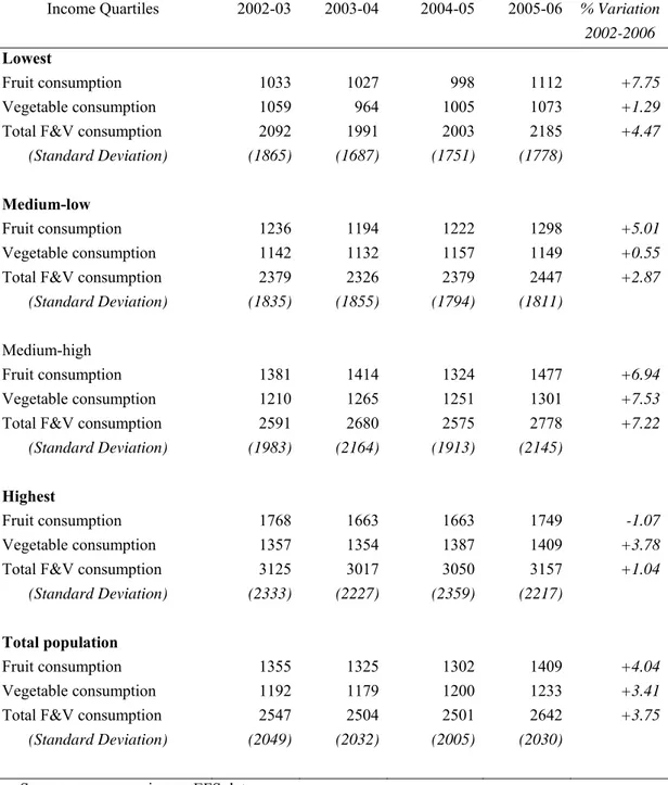
Table 3.1 shows the average per capita fruit and vegetable consumption over time, disaggregated by income quartile. Average per capita consumption is computed for every income quartile as a weighted average of per capita consumption of each household, using the sampling weights supplied with EFS data.

14 _{“One 150 ml glass of unsweetened 100% fruit or vegetable juice can count as a portion. But only one glass counts,}

further glasses of juice don’t count toward the total 5 A DAY portions” (http://www.nhs.uk/Livewell/5ADAY/Pages/FAQs.aspx)

Table 3.1 Average per capita fruit and vegetable purchases by income quartile (grams per week).

Income Quartiles 2002-03 2003-04 2004-05 2005-06 % Variation

2002-2006

Lowest

Fruit consumption 1033 1027 998 1112 +7.75

Vegetable consumption 1059 964 1005 1073 +1.29

Total F&V consumption 2092 1991 2003 2185 +4.47 (Standard Deviation) (1865) (1687) (1751) (1778)

Medium-low

Fruit consumption 1236 1194 1222 1298 +5.01

Vegetable consumption 1142 1132 1157 1149 +0.55

Total F&V consumption 2379 2326 2379 2447 +2.87 (Standard Deviation) (1835) (1855) (1794) (1811)

Medium-high

Fruit consumption 1381 1414 1324 1477 +6.94

Vegetable consumption 1210 1265 1251 1301 +7.53

Total F&V consumption 2591 2680 2575 2778 +7.22 (Standard Deviation) (1983) (2164) (1913) (2145)

Highest

Fruit consumption 1768 1663 1663 1749 -1.07

Vegetable consumption 1357 1354 1387 1409 +3.78

Total F&V consumption 3125 3017 3050 3157 +1.04 (Standard Deviation) (2333) (2227) (2359) (2217)

Total population

Fruit consumption 1355 1325 1302 1409 +4.04

Vegetable consumption 1192 1179 1200 1233 +3.41

Total F&V consumption 2547 2504 2501 2642 +3.75 (Standard Deviation) (2049) (2032) (2005) (2030)

Source: our processing on EFS data.

People in lower income quartiles consume less fruit and vegetable, a common finding in the literature (Pollard et al., 2008). In the 2002-03 baseline year, prior to the campaign kick-off, average F&V consumption for households in the richest quartile was 49% higher than for those in the lowest quartile. In 2004-05 the gap is still about 52%, with a decrease to 44% in 2005-06.

Assuming 80g per portion, and allowing 10% for wastage an estimate of the number of F&V portions consumed individually in a day has been computed (Table 3.2). Differences among income quartiles are quite evident. The richest quartile of the population seems to be on

average already in line with the recommendation of 5 portions per day (5.07 in 2005-06)15.

However the lowest income quartile is well-below the recommended threshold (3.51 portions in 2005-06).

Table 3.2 Average number of F&V portions per day by income quartile (per-capita).

Income Quartiles 2002-03 2003-04 2004-05 2005-06 Lowest

Fruit consumption 1.66 1.65 1.60 1.79 Vegetable consumption 1.70 1.55 1.62 1.72 Total F&V consumption 3.36 3.20 3.22 3.51

Medium-low

Fruit consumption 1.99 1.92 1.96 2.09 Vegetable consumption 1.84 1.82 1.86 1.85 Total F&V consumption 3.82 3.74 3.82 3.93 Medium-high

Fruit consumption 2.22 2.27 2.13 2.37 Vegetable consumption 1.94 2.03 2.01 2.09 Total F&V consumption 4.16 4.31 4.14 4.46

Highest

Fruit consumption 2.84 2.67 2.67 2.81 Vegetable consumption 2.18 2.18 2.23 2.26 Total F&V consumption 5.02 4.85 4.90 5.07

Total population

Fruit consumption 2.18 2.13 2.09 2.26 Vegetable consumption 1.92 1.89 1.93 1.98 Total F&V consumption 4.09 4.02 4.02 4.25

Another route to estimating average per capita consumption can be pursued by computing the ratio between average (weighted) household consumption and average (weighted) number of household members per each income quartile, as shown in Table 3.3. These are exactly the estimates provided by DEFRA (DEFRA, 2007) in its 2007 report on EFS food data. Yet, since our following analysis will be focused also on consumption differences among income

15 _{The issue is not of minor importance. As noted in Mazzocchi, Traill and Shogren (2009), assuming a symmetric}

distribution of fruit and vegetable consumption among the population the target of an average of 5 portions per day means that half of the population would be below the threshold. The 5-a-day message seems to require that everyone should consume five 80 grams portions per day, it follows that the average should be well-above.