ALMA constraints on the faint millimetre source number counts and their contribution to the cosmic infrared background

2020-07-06T17:46:00Z

Acceptance in OA@INAF

ALMA constraints on the faint millimetre source number counts and their

contribution to the cosmic infrared background

Title

Carniani, S.; Maiolino, R.; De Zotti, G.; Negrello, M.; Marconi, Alessandro; et al.

Authors

10.1051/0004-6361/201525780

DOI

http://hdl.handle.net/20.500.12386/26346

Handle

ASTRONOMY & ASTROPHYSICS

Journal

584

Number

October 14, 2018

ALMA constraints on the faint millimetre source number counts

and their contribution to the cosmic infrared background

S. Carniani

, R. Maiolino

, G. De Zotti

, M. Negrello

, A. Marconi

, M. S. Bothwell

, P. Capak

, C. Carilli

,

M. Castellano

_{, S. Cristiani}

_{, A. Ferrara}

_{, A. Fontana}

_{, S. Gallerani}

_{, G. Jones}

_{, K. Ohta}

_{, K. Ota}

_{, L.}

Pentericci

, P. Santini

, K. Sheth

, L. Vallini

, E. Vanzella

, J. Wagg

, R. J. Williams

3 _{Kavli Institute for Cosmology, University of Cambridge, Madingley Road, Cambridge CB3 0HA, UK} 4 _{SISSA, Via Bonomea 265, 34136, Trieste, Italy}

5 _{INAF-Osservatorio Astronomico di Padova, Vicolo dell’ Osservatorio 5, I-35122 Padova, Italy} 6 _{Spitzer Science Center, 314-6 Caltech, 1201 East California Boulevard, Pasadena, CA 91125, USA} 7 _{Department of Astronomy, 249-17 Caltech, 1201 East California Boulevard, Pasadena, CA 91125, USA} 8 _{National Radio Astronomy Observatory, P.O. Box 0, Socorro, NM 87801, USA}

9 _{INAF - Osservatorio Astronomico di Roma, via Frascati 33, 00040 Monteporzio, Italy} 10 _{INAF- Trieste Astronomical Observatory, via Tiepolo 11, 34143 Trieste, Italy} 11 _{Scuola Normale Superiore, Piazza dei Cavalieri 7, 56126, Pisa, Italy}

12 _{Physics Department, New Mexico Tech, Socorro, NM 87801, USA} 13 _{Department of Astronomy, Kyoto University, Kyoto 606-8502, Japan}

14 _{Dipartimento di Fisica e Astronomia, Universita’ di Bologna, Viale Berti Pichat 6/2, I-30127, Bologna, Italy} 15 _{INAF-Osservatorio Astronomico di Bologna, Via Ranzani 1, I-40127 Bologna, Italy}

16 _{Square Kilometre Array Organization, Jodrell Bank Observatory, Lower Withington, Macclesfield, Cheshire SK11 9DL, UK}

October 14, 2018

ABSTRACT

We have analysed 18 ALMA continuum maps in Bands 6 and 7, with rms down to 7.8 µJy, to derive differential number counts down to 60 µJy and 100 µJy at λ =1.3 mm and λ =1.1 mm, respectively. Furthermore, the non-detection of faint sources in the deepest ALMA field enabled us to set tight upper limits on the number counts down to 30 µJy. This is a factor of four deeper than the currently most stringent upper limit. The area covered by the combined fields is 9.5 × 10−4_deg2_{at 1.1 mm and 6.6 × 10}−4_deg2_{at 1.3mm. With}

respect to previous works, we improved the source extraction method by requiring that the dimension of the detected sources be consistent with the beam size. This method enabled us to remove spurious detections that have plagued the purity of the catalogues in previous studies. We detected 50 faint sources (at fluxes < 1 mJy) with signal-to-noise (S/N) > 3.5 down to 60 µJy, hence improving the statistics by a factor of four relative to previous studies. The inferred differential number counts are dN/d(Log10S)= 1×105deg2at

a 1.1 mm flux S_{λ=1.1 mm}= 130 µJy, and dN/d(Log10S)= 1.1 × 105deg2at a 1.3 mm flux Sλ=1.3 mm= 60 µJy. At the faintest flux limits

probed by our data, i.e. 30 µJy and 40 µJy, we obtain upper limits on the differential number counts of dN/d(Log10S) < 7 × 105deg2

and dN/d(Log10S) < 3×105deg2, respectively. Determining the fraction of cosmic infrared background (CIB) resolved by the ALMA

observations was hampered by the large uncertainties plaguing the CIB measurements (a factor of four in flux). However, our results provide a new lower limit to CIB intensity of 17.2 Jy deg−2_{at 1.1 mm and of 12.9 Jy deg}−2_{at 1.3 mm. Moreover, the flattening of the}

integrated number counts at faint fluxes strongly suggests that we are probably close to the CIB intensity. Our data imply that galaxies with star formation rate (SFR)< 40 M/yr certainly contribute less than 50% to the CIB (and probably a much lower percentage)

while more than 50% of the CIB must be produced by galaxies with SFR > 40 M/yr. The differential number counts are in nice

agreement with recent semi-analytical models of galaxy formation even as low as our faint fluxes. Consequently, this supports the galaxy evolutionary scenarios and assumptions made in these models.

Key words. galaxies: evolution - galaxies: formation - galaxies: high-redshift

1. Introduction

The extragalactic background light (EBL) is a diffuse and isotropic radiation in the Universe, covering the range between ultraviolet (UV) and far infrared (FIR) wavelengths (Fixsen et al. 1998). After the CMB, the EBL represents the second most ener-getic background. The IR/mm spectrum of the EBL was first es-timated by Puget et al. (1996) using data from Far Infrared Abso-lute Spectrometer on the Cosmic Background Explorer (COBE) satellite. The EBL spectral energy distribution is composed of

two peaks: the cosmic optical background (COB) and the cos-mic infrared background (CIB). The former is caused by the ra-diation from stars, while the latter is due to UV/optical light ab-sorbed by dust and reradiated in the infrared wavelength range. By measuring the integrated flux of the two components, the ra-tio between the COB and CIB is of the order of unity (Dole et al. 2006), which suggests that half of the star light emission is ab-sorbed by dust in galaxies. Therefore, the EBL contains informa-tion about star formainforma-tion processes and galaxy evoluinforma-tion in the

Universe. The study of this emission helps us to understand the star formation evolution throughout the history of the Universe.

The mixture of source populations contributing to the CIB depends strongly on the specific wavelength (e.g. Viero et al. 2013; Cai et al. 2013). At millimetre wavelengths (λ ∼ 1.1 − 1.3 µm), a significant percentage (∼ 30%) of the CIB is emitted by submillimetre galaxies (e.g. Viero et al. 2013; Cai et al. 2013). The definition of submillimetre galaxies (SMGs) is somewhat loose and is generally meant to indicate the bright end of the population of sources emitting at submm wavelengths, initially discovered by bolometers on single-dish telescopes. SMGs are predominately high-redshift (z ≥ 1) star-forming galaxies with star formation rates (SFRs) approaching 1000 Myr−1, or even

higher (e.g. Blain et al. 2002). In these galaxies, the bulk of the UV/optical emission from young stars is absorbed by the sur-rounding dust, which is re-emitted at FIR wavelengths (Casey et al. 2014). Recent studies have shown that massive red-and-dead galaxies share the same clustering properties as SMGs. Thus, SMGs may be the progenitors of local massive elliptical galaxies (Simpson et al. 2014; Toft et al. 2014).

However, SMGs represent an extreme class of objects, not representative of the bulk of the galaxy population at high z (z & 1). Most high-z galaxies show a much lower SFR and are likely associated with systems that evolve through secular pro-cesses (e.g. Rodighiero et al. 2011). For the bulk of the high-z population, the rest-frame far-IR/submm properties (which pro-vide information on obscured star formation and dust content), are still poorly known at mm/submm fluxes below 1 mJy.

In the past decades the SCUBA and LABOCA single-dish surveys resolved 20% to 40% of the CIB at 850 µm (e.g. Eales et al. 1999; Coppin et al. 2006; Weiß et al. 2009) and 10% to 20% of the CIB at 1.1 mm with deep single-dish surveys using the AzTEC camera (e.g. Scott et al. 2010). Until recently, the number counts of fainter sources (S < 1 mJy) were not well constrained because of the limited sensitivity. However, the ob-servation of lensed galaxies, hence reaching somewhat deeper flux limits (e.g. Cowie et al. 2002; Knudsen et al. 2008; Johans-son et al. 2011; Chen et al. 2013b,a) suggests that more than 50% of the CIB is emitted by faint sources with flux densities < 2 mJy.

Recently, the number counts of faint mm sources, at fluxes fainter than 1 mJy, have been inferred thanks to high-sensitivity and high-resolution observations obtained with the Atacama Large Millimeter/submillimeter Array (ALMA). Hat-sukade et al. (2013) claim to have resolved ∼ 80% ( ∼ 13 Jy deg−2) of the CIB at 1.3 mm exploring faint (0.1 - 1 mJy) sources with signal-to-noise (S/N) ≥ 4 extracted from ALMA data. A similar result has been obtained at 1.2 mm by Ono et al. (2014), who suggest that the main contribution to the CIB comes from faint star-forming galaxies with SFR < 30 M/yr. However, as

we discuss later, the uncertainties on the CIB spectrum are large, and once these are taken into account, the fraction of resolved background at these fluxes, as well as the identification of the sources contributing to the bulk of the CIB, are much more un-certain than is given in these papers. Source number counts with deep millimetre observations can provide a tight lower limit on the CIB intensity. Moreover, the slope of the faint counts con-strains contributions to the CIB from still fainter sources. Fi-nally, the detected faint millimetre sources can be targets for fu-ture spectroscopic observations aimed at understanding the prop-erties of this faint population, which is more representative of the bulk of the galaxy population than past (bright) millimeter sources.

We used imaging from ALMA with a sensitivity down to 7.8 µJy/beam (rms), which enabled us to achieve some of the faintest continuum detections at 1.1 mm and 1.3 mm with flux densities down to 60 µJy. The source counts presented here thus provide constraints on models of galaxy evolution and predictions for future ALMA follow-up surveys.

This paper is organised as follows. In Section 2, we describe the ALMA observations used in this work. Section 3 is focused on the source extraction technique. Section 4 presents the num-ber counts we derived and the comparison between our results and recent galaxy formation models. In Section 5, we discuss and summarise our results.

2. Observations and data reduction

Our source extraction is applied to 18 continuum maps with high sensitivities, which were obtained in ALMA Cycle 0 and Cycle 1. For our analysis we focused on observations in Bands 6 and 7, since these are some of the deepest observations available. In this section, we describe in detail the ALMA Bands 6 and 7 data sets used for the analysis.

The faintest sources are detected in three ALMA data sets taken by Maiolino et al. (2015), who targeted three Lyα emit-ters at z∼6-7: BDF-3299, BDF-521 and SDF-46975 (Vanzella et al. 2011; Ono et al. 2012). The BDF-3299 data (Field a in Table 1) were observed during two different epochs: a first ob-servation between October and November 2013 and a second one in April 2014. The target was observed with 27 12m an-tennae array in 2013 and 36 12m anan-tennae array in 2014 with a maximum baseline of 1270 m. The flux densities were cali-brated with the observation data of J223-3137 and J2247-3657. The total on-source integration time was ∼5.2 hr. The other two sources, BDF-521 and SDF-46975, were observed in November 2013 and March 2014, respectively, (Fields c and e in Table 1). In the extended configuration of 17-1284 m baseline for BDF-521, 29 12m antennae were used and 40 12m antennae with a maximum baseline of 422 m for SDF-46975. We used the obser-vations of J223-3137 to calibrate the flux density. The total on source observing time was about 83 min and 121 min, respec-tively, for the two targets.

We analysed nine continuum maps (fields j-r in Table 1) taken by PI Capak, who targeted [CII] emission line from sources at high redshift (z ≥ 5). The data were taken in Novem-ber 2013 using 20 antennae in band 7. The total on-source inte-gration was about 20 min for each.

We also used ALMA data (field b in Table 1) for the Lyα emitter at z= 7.215, SXDF-NB1006-2 (PI K. Ota; Shibuya et al. 2012). The target was observed on May 3-4, 2014 with a max-imum baseline of ∼ 558 m. The total on-source observing time of the 37 12 m antennae was 106 min. The flux densities were scaled with the observation data of J0215-0222.

In addition to these maps, we analysed public archival ALMA data to increase the number of detections at intermediate flux densities. We selected only continuum maps in Bands 6 and 7 with sensitivity ≤ 50 µJy/beam since we were interested in analysing the number count at flux densities < 1 mJy that con-tribute to > 60% of the CIB (Ono et al. 2014). Therefore, we analysed the data with the highest sensitivity taken by Willott et al. (2013) (Fields f and i in Table 1), Ota et al. (2014) (Field gin Table 1), MacGregor et al. (2013) (Field h in Table 1), and Ouchi et al. (2013) (Field d in Table 1). Further details on the ALMA observations are summarised in those papers.

All ALMA data were reduced using the CASA v4.2.1 pack-age. The typical flux uncertainties in the millimeter regime are

∼ 10%. The continuum maps were extracted using all the line-free channels of the four spectral windows. Unfortunately, in this version of CASA, the data weights were not set proportion-ally to the channel width and integration time, so they had to be adjusted whenever a continuum image was made from spectral windows that did not have the same channel width and index number. Furthermore, the data weights had to be fixed when a dataset was composed of different observations taken at different epochs with different integration times and different observing (water vapour) conditions. In the case of BDF-3299, BDF-521 and SDF-46975, the data weights were manually re-scaled as a function of integration time and channel width. The continuum maps were cleaned using the CASA task clean with WEIGHT-ING= “natural”, achieving a sensitivity in the range between 7.8 µJy/beam (which is the deepest ALMA observation at this wavelength and three times deeper than data used in previous studies) and 52.1 µJy/beam. The correlator of each observation was configured to provide four independent spectral windows, so the central frequency νobsin Table 1 is equivalent to the mean

frequency of the four bands. The continuum map sensitivity and the area mapped in each observation are summarised in Table 1. The source extraction was performed as far out as two primary beams, after masking the targeted source of each observation, so as not to bias the final counts determination. Around all of these sources we placed a 100_{diameter mask (∼ ALMA beam),}

since most of the main targets were non-spatially resolved. In the particular case where the main target is extended (e.g. Mac-Gregor et al. 2013), the dimension of the mask is as large as the size of the target, where the size of the target is estimated from its surface brightness emission down to 3σ. In the worst case, we masked about 5% of the field of view. The combined fields result in a total area of ∼ 9.5 × 10−4_deg2 _{at 1.1 mm and}

∼ 6.6 × 10−4_deg2 _{at 1.3 mm (which, in general, is two times}

larger than previous studies).

3. Source extraction

In total we analysed 18 ALMA continuum maps to derive the number counts of sources at millimeter wavelengths. Since we do not yet know either the spectral energy distributions (SEDs) or the redshifts of our faint mm sources, we estimated the num-ber counts at two different wavelengths, 1.1 mm and 1.3 mm, to minimise the effects of wavelength extrapolation. The flux den-sities, S , of sources detected at wavelengths less than 1.2 mm were scaled to the 1.1 mm flux density, while counts at λ> 1.2 mm were scaled to 1.3 mm using a modified blackbody with val-ues typical of SMGs at z=2. We adopted a spectral index β = 2.0 and dust temperature T = 35 K from Greve et al. (2012), who measured the SED from a sample of SMGs at the same wave-length range of our data. As these SED properties can be dif-ferent for each source, in Appendix A we estimate the errors in-duced by varying these parameters. In the following, we describe the source extraction method and the statistical assessment in de-tail.

3.1. Source catalogue

The source extraction was performed within an area as large as two primary beams that has a diameter of about 20”, before cor-recting for the primary beam attenuation. We first extracted the sources fulfilling the following requirement: 1) the source should be above the 3σ threshold in its continuum map (we then took a more conservative threshold of 3.5σ, as discussed later); 2) the

20 10 0 10 20

arcsec

arcsec

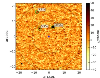
Fig. 1. Example of a Band 6 continuum map obtained with ALMA (Field a Table 1). The green circles represent the sources detected with S/N > 3.5σ that also fulfil the requirement of having a size consistent with the beam (or marginally resolved). The inner black dotted circle in-dicates the primary beam and the outer circle shows twice the primary beam. The blue filled circle shows the masked region. The synthesised beam is indicated by a filled black ellipse in the lower left corner of the plot.

size of the 2D Gaussian fitting the putative source must be con-sistent, within the errors, with the beam size of the selected map (or at most marginally resolved, within 1.5 times the beam size). Indeed, most faint sources are not expected to be spatially re-solved at the resolution of our maps. Detections with dimensions smaller than the beam must be associated with noise fluctuation of individual antennae or a group of antennae, or be caused by sidelobes of bright sources.This additional source detection cri-terion enables us to greatly reduce (by a factor of 3) the number of spurious sources, hence making the final catalogue much less prone to false detections than previous studies.

Figure 1 shows an example of an ALMA map in which the source extraction was performed down to 3σ with the above re-quirements. At this low significance level (> 3σ), some of these source candidates are likely to be spurious because of noise fluc-tuations. To define a more solid detection threshold, we esti-mated the number of spurious sources expected in the maps by applying the source extraction method to the continuum maps, which were multiplied by −1 to estimate the number of negative sources as a function of the S/N. Figure 2 shows the number of positive and negative sources as a function of S/N. The number of the negative sources is almost always less than that of the pos-itive at S/N > 3, which suggests that down to 3σ, some fraction of the positive detections are real (most of the negative sources and false positive sources are removed from the second require-ment in the source extraction process). It is also clear because the cumulative number of positive sources is larger than that of the negative ones down to S/N =3. Moreover, simulations of blank fields, with exactly the same observing conditions as our data (Appendix A), show that the number of positive and negative sources due to noise fluctuations are equal for any S/N level. Be-cause the number of positive sources was found to be larger than the number of negative ones at S/N > 3.5 in previous works from Hatsukade et al. (2013) and Ono et al. (2014), we decided to be conservative by only including those objects that satisfy the S/N > 3.5 criterion in our catalogue .

Table 1. ALMA survey fields used in this paper, sorted by sensitivity.

Project νobs σ λ Area Field

code [GHz] [µJy beam−1] [mm] [10−4deg2]

(1) (2) (3) (4) 2012.A.00040.S 230 7.8 1.28 1.17 a 2012.1.00374.S 225 14.5 1.31 1.17 b 2012.1.00719.S 230 17.7 1.30 1.17 c 2011.1.00115.S 260 18.6 1.16 0.87 d 2012.1.00719.S 244 19.5 1.23 1.06 e 2011.1.00243.S 250 20.9 1.2 0.97 f 2011.0.00767.S 230 20.9 1.30 1.17 g 2012.1.00142.S 230 26.3 1.28 1.07 h 2011.1.00243.S 249 28.9 1.2 0.97 i 2012.1.00523.S 286 29.9 1.05 0.72 j 2012.1.00523.S 295 30.0 1.02 0.71 k 2012.1.00523.S 286 30.3 1.05 0.72 l 2012.1.00523.S 289 33.1 1.05 0.72 m 2012.1.00523.S 290 36.3 1.03 0.71 n 2012.1.00523.S 289 38.1 1.05 0.72 o 2012.1.00523.S 289 41.8 1.05 0.72 p 2012.1.00523.S 292 49.1 1.02 0.71 q 2012.1.00523.S 292 52.1 1.02 0.71 r

Notes. (1) Frequency in the observed frame corresponding to the mean frequency of the four ALMA spectral window. (2) rms measured in each continuum map before primary beam correction. (3) Central wavelength in the observed frame. (4) Area in two primary beams. The size of the primary beam scales linearly with wavelength.

In the 18 continuum maps, we detected 50 sources with S/N in the range 3.5-38.4, and none of them appear to be marginally resolved. These statistics are a factor of four higher than previous studies (Ono et al. 2014).

3.2. Completeness and survey area

For each ALMA map i, we estimated the completeness, Ci(S ),

which is the expected probability at which a real source with flux S can be detected within the entire field of view that we consid-ered (i.e. two primary beams). The Ci(S ) is calculated in each

ALMA map corrected for primary beam attenuation. To esti-mate the completeness we inserted artificial sources with a given flux density S (at which we want to estimate the completeness). The positions of these artificial sources are randomly distributed within the two primary beams. The input source is considered re-covered when it is extracted with S/N≥ 3.5σ. Within the selected flux densities range (0.05 to 1 mJy) we iterated the procedure of inserting artificial sources for each continuum map 1000 times, using four to eight artificial sources in each simulation for each field. The completeness calculated in each map, Ci(S ), is equal

to the ratio between the number of recovered sources and the number of input sources for each flux S . Figure 3 shows Ci(S )

as a function of the intrinsic flux density S , estimated on the deepest ALMA continuum map (Field a in Table 1).

The beam response is not uniform and decreases with in-creasing distance from the map centre. Therefore, the effective area that is sensitive to a given flux S decreases rapidly with the flux itself. As a consequence, the effective area of the survey depends on the considered flux, i.e. Asurvey(S ). Since the

com-pleteness Ci(S ) is estimated on the continuum maps that have

been corrected for primary beam attenuation, the completeness function already automatically includes the effect of variation of sensitivity as a function of distance from the map centre. There-fore, the effective survey area of each map at a given flux S is

given by Ci(S )Ai(S ), where Ai(S ) is the two-primary-beam area

of the ALMA map i. Therefore, the total effective survey area is given by

Asurvey(S )=

X

i

Ci(S )Ai(S ) .

We obtained Asurvey(S ) both at 1.1 mm and at 1.3 mm, as

shown in Figure 4.

3.3. Flux boosting

The noise fluctuations in continuum maps may influence photo-metric measurements of the extracted sources. Since the counts of faint sources increase with decreasing flux density (e.g. Scott et al. 2012; Hatsukade et al. 2013; Ono et al. 2014), there should be a ‘sea’ of faint source below the noise level that may influ-ence photometric extraction. There is, indeed, a greater proba-bility that intrinsically faint sources are detected at higher flux, rather than that bright ones are de-boosted to a lower flux. (See Hogg & Turner (1998) and Coppin et al. (2005) for a full de-scription of this effect.) This effect, called flux boosting, is ex-tremely important at low S/N (< 5) where flux measurement can be overestimated. Since we do not know the priori distribution of flux densities in the range 0.001-1 mJy, we performed a sim-ple simulation to estimate the boost factor as a function of S/N detection.

The simulation was carried out in the map that was uncor-rected for primary beam attenuation. Into the maps we inserted flux-scaled artificial sources (4-8) whose S/N are in the range of 3-8. Then, we extracted the flux densities at the same position where the sources were located. The a priori knowledge of the source position in this process may lead to underestimating the flux boosting correction since the noise in the maps may lead to an offset in the recovered position of mock (or real) sources.

3.0 3.5 4.0 4.5 5.0 5.5 6.0 6.5 7.0

S/N

0

5

10

15

20

25

30

35

40

number of detections

10

21.4

38.6

3.0 3.5 4.0 4.5 5.0 5.5 6.0 6.5 7.0 7.5

S/N

20

40

60

80

100

120

140

number of detections > S/N

Fig. 2. Top: number of positive (red) and negative (blue) sources de-tected in the 18 continuum maps, as a function of S/N. Bottom: cumu-lative distribution of positive (red) and negative (blue) detections.

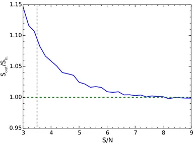
However this effect is maximum when sources are near a noise peak. Since the number of mock (or real) sources in each contin-uum map is low (<10), the probability that an artificial (or real) source is near to a noise peak is lower than 5%. In conclusion, the error on the flux-boosting factor, which is due to the a priori knowledge of artificial source position, is small (< 5%). The flux boosting is calculated as the ratio of the measured flux density (Sout) to the input flux density (Sin). We repeated this simulation

for each ALMA continuum map 104 times. Figure 5 shows the average ratio of the extracted flux densities Soutto the input flux

densities Sinas a function of S/N. At S/N = 3.5, the boost

frac-tion is '1.09, so the difference between extracted flux and input flux is less than 10%. The boosting factor correction (Figure 5) was then applied to the measured detection fluxes.

4. Results

To summarise the previous sections, we detected 50 sources with S/N > 3.5 in 18 continuum maps in the ALMA Bands 6 and 7. Then, we corrected the flux densities for the flux-boosting effect. In the following, we discuss the additional steps required to infer the sources’ number counts and the comparison with the CIB.

0

100 200 300 400 500 600 700 800 900

intrisic flux density [ Jy]

0.2

0.4

0.6

0.8

1.0

co

m

ple

tn

es

s C

(S

)

Fig. 3. Completeness Ci(S ) as a function of the flux density S , estimated

from simulations. The solid curve is the result for field a with rms= 7.8 µJy/beam.

100 200 300 400 500 600 700 800 900

flux denisty [ Jy]

0.0

0.2

0.4

0.6

0.8

1.0

1.2

su

rv

ey

ar

ea

[1

0

d

eg

]

1.1mm

1.3mm

Fig. 4. Effective survey area as a function of intrinsic flux density. This is the area over which a source with an intrinsic flux density S can be detected with S /N > 3.5σ. The blue and green curves are the survey areas for the maps at 1.1 mm and 1.3 mm, respectively.

4.1. Differential number counts

We scaled the flux density of the sources observed at λ < 1.2 mm to the flux density at 1.1 mm and those at λ > 1.2 mm to the flux density at 1.3 mm. The reason for splitting the sources into these two wavelength ranges is that this significantly reduces the un-certainties on the flux obtained from the extrapolation. A more detailed analysis of these issues is given in Appendix B. With this strategy, the error on the flux associated with each source is always less than 18%. Following the prescription of Hatsukade et al. (2013) and Ono et al. (2014), we estimated the number counts at two different wavelengths: 1.1 mm and 1.3 mm. We then estimated the effective survey area associated with the flux of each source. To estimate the number counts, we corrected for the contamination of ‘spurious’ sources, i.e. the fraction of sources that are due to noise fluctuations above the 3.5σ level (and meeting the additional requirements given in sect 3.1). The contamination fraction fcwas inferred from the fraction of

neg-3

4

5

6

7

8

9

S/N

0.95

1.00

1.05

1.10

1.15

S

/S

Fig. 5. Flux-boosting factor as a function of S/N, estimated from sim-ulations. The horizontal dashed line corresponds to Sout = Sin . The

vertical dashed line corresponds to the detection threshold, S/N = 3.5.

ative sources at each S/N level, as inferred from Figure 2. For each source, fcis the ratio between negative and positive

detec-tions at its S/N. Therefore, the contribution of each source to the number counts is (1- fc) divided by its respective effective

sur-vey area Asurvey(S ). We carried out the logarithmic differential

number counts dN(S )/dLogS in logarithmic flux density bins with size∆LogS = 0.2. So the logarithmic differential number counts for a selected bin is given by

dN(S ) dLogS     _{S ±1/2∆LogS} = X j 1 − fc j Asurvey(S ) ,

where j are all sources with flux density between LogS -1/2∆LogS and LogS +1/2∆LogS . The resulting differential number counts are scaled to∆LogS = 1.

The total uncertainty on the logarithmic differential number counts is computed by combining the contribution from Poisson noise, from the cosmic variance and from errors due to complete-ness and flux-boosting corrections. In the following we evaluate each single contribution:

◦ The observational uncertainty related to the actual number of detected sources is calculated from Poisson confidence limits of 84.13% (Gehrels 1986) by using the number of sources detected in each bin.

◦ The error due to the cosmic variance is estimated by us-ing a software tool provided by Moster et al. (2011). This procedure uses predictions of the underlying structure of cold dark matter and the expected bias for a galaxy popu-lation. The estimate depends on the angular dimension of the field, the mean redshift, the redshift bin size, stellar mass of the galaxy population in question, and also on the num-ber of independent fields sampled in different regions of the sky. We assume a mean redshift of z = 3.5, a redshift bin size of dz = 3, and a stellar mass of 1010.5 M from Yun

et al. (2012) and Weiß et al. (2013) who measured and anal-ysed SEDs and redshifts of bright (S>1mJy) submillime-tre galaxies through spectroscopic and photometric observa-tions. Considering that for widely separated fields the cosmic variance goes as 1/√Nfield, the relative error is < 18% in the

deepest logarithmic differential number count bin.

Table 2. Differential number counts. λ = 1.1 mm S [mJy] dN/dLog(S ) [104_{] N} detections 0.13 10+7₋₄ 5 0.20 11+3₋₃ 14 0.30 2+2₋₁ 3 0.63 0.7+0.9_−0.4 2 λ = 1.3 mm

S [mJy] dN/dLog(S ) [104] Ndetections

0.03 <70 -0.04 <30 -0.06 11+14₋₇ 2 0.08 10+7₋₄ 5 0.12 7+4₋₃ 7 0.22 3+2₋₂ 5 0.34 4+2₋₂ 7

◦ The relative uncertainties relating to completeness and flux-boosting corrections of the order of 5%.

Because the cosmic variance and errors induced by count esti-mations (completeness, flux boosting) are less than 20%, the un-certainty on logarithmic differential number counts is completely dominated by the Poisson errors.

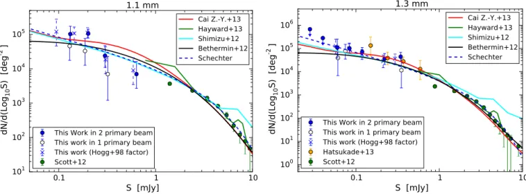
The resulting differential number counts are summarised in Table 2 and shown in Figure 6 (blue solid symbols). Number counts could be derived down to 60µJy at 1.3mm and down to 100µJy at 1.1mm. Moreover, since we do not detect any faint sources with flux densities 30 . S . 50 µJy in the deepest ALMA map (Field a in Table 1) with sensitivity of ∼ 7.8 µJy, we can set a tight upper limit on the number counts at S= 30 µJy and at S= 40 µJy. We note that, with the latter, we constrain the number counts at flux levels that are a factor of four deeper than previous studies (Ono et al. 2014). We also show separately (hollow symbols) the number counts inferred by only using the sources detected within the primary beam (i.e. 7 sources at 1.1 mm and 6 sources at 1.3 mm). In the latter case, the statistical errorbars are obviously larger but fully consistent (within errors) with the number counts inferred over two beams.

We also show the number counts of bright (S> 1 mJy) SMGs obtained by Scott et al. (2012) at 1.1 mm with AzTEC. However, the two faintest bins in the latter data are not considered when comparing models or when fitting analytic functions since the completeness at these flux densities is too low and the number counts are underestimated. Since there are no number counts of bright sources at 1.3 mm, we used the number counts at 1.1 mm by scaling the flux density to 1.3 mm flux density. Figure 6 shows that the differential number counts increase with decreasing flux density. At 1.3 mm, the differential number counts of Hatsukade et al. (2013) (orange symbols), which are obtained from sources with S/N≥ 4, are consistent with our results within the uncertain-ties, but our slope of the logarithmic number counts at sub-mJy flux densities is flatter than those obtained by Hatsukade et al. (2013). We do not plot the number counts of Ono et al. (2014) as they were estimated at 1.2 mm using continuum maps over the whole 1.04-1.22 mm wavelength range, i.e. they were not extracted with the same procedure we used to define our sam-ple. Given that there is no information yet on the SED or on the redshift of the sources contributing to the number counts, our

0.1

1

10

S [mJy]

10

10

10

10

10

d

N/

d(

Lo

g

S)

[

de

g

]

1.1 mm

This Work in 2 primary beam This work in 1 primary beam This work (Hogg+98 factor) Scott+12 Cai Z.-Y.+13 Hayward+13 Shimizu+12 Bethermin+12 Schechter

0.1

1

10

S [mJy]

10

10

10

10

10

10

10

d

N/

d(

Lo

g

S)

[

de

g

]

1.3 mm

This Work in 2 primary beam

This work in 1 primary beam

This work (Hogg+98 factor)

Hatsukade+13

Scott+12

Cai Z.-Y.+13

Hayward+13

Shimizu+12

Bethermin+12

Schechter

Fig. 6. Logarithmic differential number counts as a function of flux density at λ =1.1 mm and λ =1.3 mm. The blue solid and upper limit symbols are the results of this work. The hollow symbols are the results obtained by using only the sources within one primary beam. The blue crosses with dashed error bars are the differential number counts corrected for flux boosting by using Equation 4 in Hogg & Turner (1998). The green symbols are estimated from Scott et al. (2012). The orange symbols are the number counts estimated by Hatsukade et al. (2013). The red, green, cyan, and black solid curves are the model predictions obtained by Cai et al. (2013), Hayward et al. (2013), Shimizu et al. (2012), and Béthermin et al. (2012), respectively. The blue dashed curve shows the best-fit Schechter function.

approach of dividing sources into two wavelength ranges, hence minimising the extrapolation assumptions, provides more solid results, as discussed in more detail in Appendix B.

Since some previous works assess the boosting factor cor-rection by using a Bayesian estimation (e.g. Coppin et al. 2005) instead of that shown in Sec. 3.3, we verified that the final results do not depend on the method used to correct the flux-boosting ef-fect. Therefore, we show (with crosses and dashed error bars) the differential number counts by correcting for a boost factor that is estimated from Equation (4) of Hogg & Turner (1998) (note that the correction was on the data not corrected for flux boosting as described in Sect. 3.3, otherwise this would result in a double correction). To apply the prescription of Hogg & Turner (1998), we used the best-fit Schechter function (Sect. 4.3) as a conserva-tive a priori distribution of flux densities at faint fluxes (we shall see that a Schechter function tends to give an extrapolation of the number counts that is steeper than expected for models and tends to overproduce the CIB). It should, however, be noted that the prescription given by Hogg & Turner (1998) may not apply to these data, since the noise is not uniformly distributed over the field of view as a consequence of the primary beam attenua-tion. However, as seen in Figure 6, the slopes obtained with this correction factor are consistent with those obtained using a boost factor estimated in Sec. 3.3.

We also note that, while this paper was under review, a paper was posted on arXiv in which differential number counts down to 20µJy are estimated by exploiting data on a lensing cluster (Fuji-moto et al. 2015). Their claimed number counts at 20-40µJy are significantly higher then the upper limits estimated by us on un-lensed sources. We tentatively ascribe the discrepancy to uncer-tainties associated with the calculation of the lensing factor for sources of unknown redshift and to uncertainties associated with the complex calculation of the effective survey area in the pres-ence of strong lensing. However, new forthcoming deep ALMA observations will enable us to clarify these discrepancies further.

4.2. Comparison with models

We compared the differential and integrated number counts to the theoretical results obtained by recent simulations and semi-analytical models. In Figure 6, the differential number counts by Hayward et al. (2013) are shown with a green line. Their re-sults were obtained by combining a semi-analytical model with 3-D hydrodynamical simulations and 3-D dust radiative transfer calculations. The main contributions to the mm counts is from isolated-disc, galaxy pairs, and late-stage merger-induced star-bursts. Figure 6 shows that their model predictions are able to reproduce the observational results at flux densities > 2 mJy,

We also compared our results with the model by Shimizu et al. (2012), who performed cosmological hydrodynamics sim-ulations using an updated version of the Tree-PM smoothed par-ticle hydrodynamics code, GADGET-3. They assume feedback mechanisms were triggered by supernovae and the SED of galax-ies at mm-FIR wavelengths were described by a modified black body emission. This model predicts that the bright SMGs reside in greater massive halos (> 1012M) and that their typical

stel-lar masses are greater than 1011 _M

. Their results are broadly

consistent with the ALMA results up to 1–5 mJy. However, their estimated number counts of bright SMGs (> 1 − 5 mJy) are sig-nificantly higher than the observed number counts, both at 1.1 and 1.3 mm. According to this model, approximately 90% of millimeter sources in the flux range of 0.1-1 mJy are at z > 2. Therefore, most of the observed sources are high-z galaxies and the contribution from low-z is small.

Béthermin et al. (2012) developed an empirical model in which they start from mid-IR and radio number counts, and by using a library of SEDs, they predict the number counts at far-IR and millimeter wavelengths. This model is based on a redshift evolution of the SEDs associated with the two star formation modes: main-sequence and starburst. The predictions of their empirical model are plotted as solid black curves in both panels of Figure 6. Their corresponding SEDs are derived from Her-schel observations. The predictions are slightly below the ob-served faint-end, both at 1.1 mm and 1.3 mm. However, the gen-erally good matching of the model with the observations

sug-gests that the faint millimeter sources (S < 1mJy) are more likely associated with normal (main sequence) star-forming galaxies, since the starburst emission dominates at higher flux densities at these wavelengths.

Finally, Figure 6 shows the theoretical predictions of Cai et al. (2013)1. The Cai et al. (2013) model starts by consider-ing the observed dichotomy in the ages of stellar populations of massive spheroidal (components of) galaxies on one side and late-type galaxies on the other. Spheroidal galaxies and massive bulges of Sa-type galaxies must have formed most of their stars at z & 1, while the disc components of spirals and the irreg-ular galaxies are characterised by significantly younger stellar populations, with star-formation activity continuing up to the present time. The model includes a self-consistent treatment of the chemical evolution of the ISM, calculated using the standard equations and stellar nucleosynthesis prescriptions. The chemi-cal evolution controls the evolution of the dust abundance, hence the dust absorption and re-emission. On the other hand, the evo-lution of late-type galaxies was described using a phenomeno-logical approach and considering two populations with di ffer-ent SEDs and different evolutionary properties: ‘normal’ late-type galaxies, with low evolution and low dust temperatures (‘cold’ population) and rapidly evolving starburst galaxies, with warmer dust temperatures (‘warm’ population). Their results are in good agreement with our differential number counts from faint to bright flux densities at 1.3 mm and also 1.1 mm (although with some deviations). According to this model the steep slope of the bright counts is accounted for by the sudden appearance of star-forming proto-spheriodal galaxies at z & 1.5, whose counts al-ready begin to flatten at flux densities of a few-to-several mJy’s. The counts of starburst galaxies have a somewhat flatter slope and come up at levels similar to those of proto-spheroids at the flux densities of the (new) faint counts, while the contribution of ‘normal’ late-type galaxies is always minor in the consid-ered flux density range but increases with decreasing flux den-sity. The redshift distribution at the flux densities of the present counts is bimodal, with starburst galaxies peaking at z ' 1.5 and proto-spheroids peaking at z ' 2. At bright flux densities (S ∼ 10 mJy), the starburst galaxy peak shifts to z  1 (being the brightest, in flux terms, starburst galaxies are mostly local) while the proto-spheroid one remains at z ' 2.

4.3. Source counts parametrisation with a Schechter function We also parametrised the differential number counts using a Schechter function: dN dSdS = φ? S S? !α exp −S S? ! d S S? ! ,

with φ?being the normalisation, S?the characteristic flux den-sity, and α the faint-end slope of the number counts. We fitted the Schechter function separately at 1.1 mm and 1.3 mm by using the number counts estimated in this work and from the literature (e.g. Scott et al. 2012, Hatsukade et al. 2013). We did not use the two faintest data points from Scott et al. (2012) because they may suffer from completeness problems. The three free param-eters were then derived by χ2 minimisation. Table 3 reports the best-fit parameters and Figures 6 and 7 show the results of the Schechter function fitting.

The reduced χ2_{are 0.9 at 1.1 mm and 1.1 at 1.3 mm,}

mean-ing that the differential number counts can be properly described

1 _{The models predictions are available in electronic format at the Web}

site http://staff.ustc.edu.cn/∼zcai/

Table 3. Best-fit parameters of the Schechter function at λ =1.1„ and λ =1.3mm.

λ φ?[deg−2] S?[mJy] α

1.1 mm (2.7 ± 0.9) × 103 _{2.6 ± 0.4 −1.81 ± 0.14}

1.3 mm (1.8 ± 0.4) × 103 _{1.7 ± 0.2 −2.08 ± 0.11}

by a Schechter function down to the flux levels observed by us. The two faint-end slopes are similar within the errors, suggesting that the two number counts can be described by the same func-tion. The bright-end shape also matches with a pure Schechter function perfectly well at both wavelengths, which has recently been observed in Dayal et al. (2014).

However, we note that the slope of the Schechter function is significantly steeper than expected by models (especially at 1.3 mm) and would overproduce the CIB at faint fluxes, even taking the upper boundary of the CIB, which is discussed in the next section. Therefore, we warn that the Schechter function fitted to the current data is probably not suitable for describing the number counts at fluxes fainter than those observed by us. 4.4. Cosmic infrared background

We calculated the 1.1 mm and 1.3 number counts down to 60 µJy using Cycle 0 and 1 ALMA observations. Using the improved number counts estimated in this work, we estimated the inte-grated flux densities from resolved sources and we derived the fraction of the CIB resolved by ALMA at 1.1 mm and 1.3 mm. The integrated flux densities are given by

I(S > Slim)= Z ∞ Slimit dN(S ) dS S dS, where dN(S ) dS = dN(S ) dLogS 1 Sln(10).

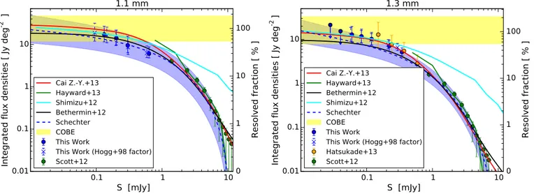
Figure 7 shows the integrated flux densities at 1.1 mm and 1.3 mm as a function of Slimit. We note that we used the results

of Scott et al. (2012) at bright flux (S > 1mJy), but excluding the two point at faintest fluxes, because of incompleteness issues. The integrated counts down to Slimit= 0.1 mJy at 1.1 mm and to

Slimit= 0.06 mJy at 1.3 mm are 17+10₋₅ Jy deg−2and 13+6−3Jy deg −2

respectively. We compared these results with the analytical fit obtained by Fixsen et al. (1998) from the COBE measurement: 25+22₋₁₃ Jy deg−2 at 1.1 mm and 17+16₋₉ Jy deg−2 at 1.3 mm (see also Lagache et al. 1999 and Schmidt et al. 2015). Since these measurements suffer from large uncertainties (especially due to the uncertainties on the Galactic contribution), we are not able to exactly determine the fraction of CIB resolved. Certainly, even by taking the highest value of the CIB that is consistent with the uncertainties given by Fixsen et al. (1998), we can say that at 60µJy more than 50% (but probably much more) of the CIB is resolved. Thus our results provide a lower limit on the CIB intensity at 1.1 mm and 1.3 mm. Moreover, the flatness of the faint end-slopes, in particular the flatness at 1.3 mm, suggests that the integrated flux densities estimated in this work are likely to be close to the CIB intensity.

The blue curve gives the integrated number counts inferred from the Schechter function that fit the differential number counts, and the shaded blue area gives the associated uncertainty. The uncertainty of the latter is large enough to be consistent with

0.1

1

10

S [mJy]

0.01

0.1

1

10

Int

eg

ra

te

d

flu

x d

en

sit

ies

[

Jy

de

g

]

This Work (Hogg+98 factor) Scott+12

0

1

10

100

Resolved fraction [ % ]

1.1 mm

0.1

1

10

S [mJy]

0.01

0.1

1

10

Int

eg

ra

te

d

flu

x d

en

sit

ies

[

Jy

de

g

]

This Work (Hogg+98 factor) Hatsukade+13 Scott+12

0

1

10

100

Resolved fraction [ % ]

1.3 mm

Fig. 7. Integrated flux density at λ =1.1 mm and λ =1.3 mm. The right axis shows the fraction of resolved CIB. The yellow shaded region is the CIB measured by COBE (Puget et al. 1996; Fixsen et al. 1998). The blue symbols are the results from this work (we used the differential number counts by Scott et al. (2012), indicated by green symbols for S > 1mJy ). The blue crosses with dashed error bars are the results from this work, corrected for the flux boosting, using Equation 4 in Hogg & Turner (1998). The orange symbols are from the number counts estimated by Hatsukade et al. (2013). The red, green, cyan, and black solid curves are the model predictions by Cai et al. (2013), Hayward et al. (2013), Shimizu et al. (2012), and Béthermin et al. (2012), respectively. The blue dashed curve shows the integrated flux densities estimated from the best-fit Schechter function, and the blue shaded region indicates its statistical uncertainty.

any value of the CIB within the range given by Fixsen et al. (1998), however the slope would indicate that this functional form would saturate even the highest boundary at the CIB at faint fluxes, as discussed above.

We note that the integrated number counts show a clear tening at lowest flux bins populated by our detections. The flat-tening of the number counts is supported by the tight upper limits at the faintest fluxes sampled by us. Such flattening of the num-ber counts, fully consistent with the models, suggests that we are actually resolving most of the CIB at our faint fluxes.

It will be of great interest to investigate, with followup ob-servations, what the redshift distribution is of these sources that produce most of the background, especially at the faint end. In the meantime, we can infer what the properties are of these galaxies in terms of SFR. Indeed, because of the negative K-correction, at 1.3mm a given observed flux density corresponds to an IR-luminosity (hence a SFR) that is nearly independent of redshift, across the entire redshift range 0.5< z <15 (by adopt-ing the conversion factor and IMF given in Blain et al. 1999; Maiolino et al. 2008). In particular, the minimum flux density sampled by us, 60 µJy at 1.3mm, corresponds to a total IR lu-minosity L(8 − 1000µm) = 6 × 1044 _{erg s}−1_{, corresponding}

to a SFR = 40 M yr−1 (Kennicutt & Evans 2012), nearly

in-dependent of redshift. This is consistent with the predictions of Béthermin et al. (2012) and Cai et al. (2013) as they expect faint sources to be associated with ‘normal’ star-forming galaxies. We can therefore state that galaxies with SFR < 40 M yr−1

cer-tainly contribute less than 50% of the CIB at 1.3 mm, and prob-ably a much lower percentage. Vice versa, the bulk of the CIB (50% and probably much more) must be due to galaxies with SFR > 40 Myr−1.

5. Summary and conclusions

We have used 18 deep ALMA maps in Bands 6 and 7 to in-vestigate the number counts of sources at millimeter wave-lengths. The sensitivity (rms) of these ALMA maps range from 7.8 µJy/beam to 52 µJy/beam.

Sources were detected down to 3.5σ. As a requirement for detection, we applied that the size of the sources should be equal to the beam size (or slightly larger) within the uncertainties. Since the noise due to bad UV-visibilities, or to sidelobes emis-sions from bright sources, or to thermal noise associated with in-dividual antennae or group of antennae should introduce fluctu-ations that have a spatial shape that is completely different from the coherent beam, this criterion enables us to remove most of the spurious detections associated with noise fluctuations.

We searched for sources out to a distance equal to the di-ameter of two primary beams. However, we have checked that the final number counts do not change, within errors, by restrict-ing the source search to within the primary beam (although the statistics are obviously lower).

A total of 50 sources were detected that match these cri-teria. We explored counts at these two different wavelengths, 1.1mm and 1.3mm (hence the ALMA maps were divided into two groups, depending on their central wavelength). This ap-proach avoids large flux extrapolation from observations ob-tained at different wavelengths. Since we do not yet know the intrinsic SED and redshift distribution of the detected sources (which would be required for a proper extrapolation of the fluxes from different wavelengths), our approach provides safer results, although at the expense of lower statistics.

Number counts were obtained by taking into account com-pleteness, flux-boosting effects, correction for spurious sources, and an effective survey area at different flux limits. We extracted differential number counts down to 60 µJy and 100 µJy at 1.3mm and 1.1mm, respectively, inferring sources’ number densities of dN/d(LogS ) ∼ 105_deg−2_{at these faint limits. Using the deepest}

ALMA field, we inferred tight upper limits on the number counts at 30 µJy and at 40 µJy.

The differential number counts at 1.1mm (1.3mm), across the entire range from 60 µJy to 10 mJy, can be fitted with a Schechter function with a faint end slope α ≈ −1.8 (α ≈ −2.0), a charac-teristic flux density S∗≈ 2.6 mJy (S∗ ≈ 1.7 mJy), and a

normal-isation at S∗of φ∗= 2.7 × 103deg−2(φ∗= 1.8 × 103deg−2). We

down to 60–100 µJy, but their extrapolation to fainter fluxes is not trustworthy.

The large uncertainties affecting our knowledge of the CIB level prevents us from setting tight limits on the fraction that is resolved by our data. Clearly, at least 50% of the CIB is resolved by our data (and probably much more). However, our results set a lower limit to the CIB intensity at 1.1-1.3 mm, significantly above the one coming from direct measurements. The flatness of the faint counts implies that this lower limit is likely to be close to the CIB intensity.

The SFR of the sources contributing to the CIB at such faint fluxes is about 40 M yr−1, independent of their redshift. We

therefore infer that sources with SFR < 40 Myr−1 contribute

less than half of the CIB at 1.3 mm, and probably much less. Conversely, the bulk of the CIB must be produced by galaxies with SFR > 40 Myr−1.

Acknowledgements. We thank the anonymous referee for comments and suggestions that improved the paper. We thank Paola Andreani, Matthew Auger and Valentina Calvi for comments and discussions. This paper makes use of the following ALMA data: ADS/JAO.ALMA#2011.1.00115.S, ADS/JAO.ALMA#2011.1.00243.S, ADS/JAO.ALMA#2011.1.00767.S, ADS/JAO.ALMA#2012.1.00142.S, ADS/JAO.ALMA#2012.1.00374.S, ADS/JAO.ALMA#2012.1.00523.S, ADS/JAO.ALMA#2012.1.00719.S and ADS/JAO.ALMA#2012.A.00040.S. ALMA is a partnership of ESO (repre-senting its member states), NSF (USA) and NINS (Japan), together with NRC (Canada) and NSC and ASIAA (Taiwan), in cooperation with the Republic of Chile. The Joint ALMA Observatory is operated by ESO, AUI/NRAO and NAOJ. GDZ and MN acknowledge financial support from ASI/INAF Agreement 2014-024-R.0 for the Planck LFI activity of Phase E2.

References

Béthermin, M., Daddi, E., Magdis, G., et al. 2012, ApJ, 757, L23 Blain, A. W., Moller, O., & Maller, A. H. 1999, MNRAS, 303, 423

Blain, A. W., Smail, I., Ivison, R. J., Kneib, J.-P., & Frayer, D. T. 2002, Phys. Rep., 369, 111

Cai, Z.-Y., Lapi, A., Xia, J.-Q., et al. 2013, ApJ, 768, 21

Casey, C. M., Narayanan, D., & Cooray, A. 2014, Phys. Rep., 541, 45 Chen, C.-C., Cowie, L. L., Barger, A. J., et al. 2013a, ApJ, 762, 81 Chen, C.-C., Cowie, L. L., Barger, A. J., et al. 2013b, ApJ, 776, 131 Coppin, K., Chapin, E. L., Mortier, A. M. J., et al. 2006, MNRAS, 372, 1621 Coppin, K., Halpern, M., Scott, D., Borys, C., & Chapman, S. 2005, MNRAS,

357, 1022

Cowie, L. L., Barger, A. J., & Kneib, J.-P. 2002, AJ, 123, 2197

Dayal, P., Ferrara, A., Dunlop, J. S., & Pacucci, F. 2014, MNRAS, 445, 2545 Dole, H., Lagache, G., Puget, J.-L., et al. 2006, A&A, 451, 417

Eales, S., Lilly, S., Gear, W., et al. 1999, ApJ, 515, 518

Fixsen, D. J., Dwek, E., Mather, J. C., Bennett, C. L., & Shafer, R. A. 1998, ApJ, 508, 123

Fujimoto, S., Ouchi, M., Ono, Y., et al. 2015, ArXiv e-prints [arXiv:1505.03523]

Gehrels, N. 1986, ApJ, 303, 336

Greve, T. R., Vieira, J. D., Weiß, A., et al. 2012, ApJ, 756, 101

Hatsukade, B., Ohta, K., Seko, A., Yabe, K., & Akiyama, M. 2013, ApJ, 769, L27

Hayward, C. C., Narayanan, D., Kereš, D., et al. 2013, MNRAS, 428, 2529 Hogg, D. W. & Turner, E. L. 1998, PASP, 110, 727

Johansson, D., Sigurdarson, H., & Horellou, C. 2011, A&A, 527, A117 Kennicutt, R. C. & Evans, N. J. 2012, ARA&A, 50, 531

Knudsen, K. K., van der Werf, P. P., & Kneib, J.-P. 2008, MNRAS, 384, 1611 Lagache, G., Abergel, A., Boulanger, F., Désert, F. X., & Puget, J.-L. 1999,

A&A, 344, 322

MacGregor, M. A., Wilner, D. J., Rosenfeld, K. A., et al. 2013, ApJ, 762, L21 Maiolino, R., Carniani, S., Fontana, A., et al. 2015, MNRAS, 452, 54 Maiolino, R., Nagao, T., Grazian, A., et al. 2008, A&A, 488, 463

Moster, B. P., Somerville, R. S., Newman, J. A., & Rix, H.-W. 2011, ApJ, 731, 113

Ono, Y., Ouchi, M., Kurono, Y., & Momose, R. 2014, ApJ, 795, 5 Ono, Y., Ouchi, M., Mobasher, B., et al. 2012, ApJ, 744, 83 Ota, K., Walter, F., Ohta, K., et al. 2014, ApJ, 792, 34 Ouchi, M., Ellis, R., Ono, Y., et al. 2013, ApJ, 778, 102

Puget, J.-L., Abergel, A., Bernard, J.-P., et al. 1996, A&A, 308, L5 Rodighiero, G., Daddi, E., Baronchelli, I., et al. 2011, ApJ, 739, L40

Schmidt, S. J., Ménard, B., Scranton, R., et al. 2015, MNRAS, 446, 2696 Scott, K. S., Wilson, G. W., Aretxaga, I., et al. 2012, MNRAS, 423, 575 Scott, K. S., Yun, M. S., Wilson, G. W., et al. 2010, MNRAS, 405, 2260 Shibuya, T., Kashikawa, N., Ota, K., et al. 2012, ApJ, 752, 114 Shimizu, I., Yoshida, N., & Okamoto, T. 2012, MNRAS, 427, 2866 Simpson, J. M., Swinbank, A. M., Smail, I., et al. 2014, ApJ, 788, 125 Toft, S., Smolˇci´c, V., Magnelli, B., et al. 2014, ApJ, 782, 68 Vanzella, E., Pentericci, L., Fontana, A., et al. 2011, ApJ, 730, L35 Viero, M. P., Moncelsi, L., Quadri, R. F., et al. 2013, ApJ, 779, 32 Weiß, A., De Breuck, C., Marrone, D. P., et al. 2013, ApJ, 767, 88 Weiß, A., Kovács, A., Coppin, K., et al. 2009, ApJ, 707, 1201 Willott, C. J., Omont, A., & Bergeron, J. 2013, ApJ, 770, 13 Yun, M. S., Scott, K. S., Guo, Y., et al. 2012, MNRAS, 420, 957

Appendix A: ALMA noise fluctuations

In Sec. 4.1, we have defined fcas the ratio between negative and

positive detections and we have estimated how fcdepends on the

S/N of our observations. Since this study shows that some of the real sources can be spurious because of noise fluctuations, we further verify the reliability of our catalogue in this Appendix by estimating the fcvalue expected in blank fields observed with

ALMA. In a pure blank field, the positive and negative sources are only caused by noise fluctuation, so we expect fc∼ 1 at any

S/N level.

We used the simobserve CASA v.4.2.1 task to produce syn-thetic interferometric observations of a blank field placed at the RA= 22:28:12.28 and DEC = -35:089:59.6, which are the coor-dinates of the deepest continuum map (Field a Table 1). As for the CASA input, we required that antenna configuration would be the same as those used during the observations. Furthermore, we added a thermal noise component by setting the parameter thermal noise to tsys-atm with a precipitable water vapour of 1.1 mm and ambient temperature of 269 K, which are typical values of our observations. We simulated 300 continuum maps chang-ing each time the parameter seed with a random value, which allows us to generate a random thermal noise for each observa-tion.

We then applied the source extraction technique, mentioned in Section 3.1, on each mock continuum map. Figure A.1 shows the number of positive and negative sources as a function of S/N normalised to 18 continuum fields. The number of negative sources is equal to those of positive ones at any S/N, indicating that the number of positive and negative spurious sources due to noise fluctuations is equal ( fc∼ 1 for each S/N).

Since the number of spurious positive sources is almost equal to negative ones in a blank field, most of the positive sources detected in our observations with S/N> 3 (Fig. 2) are likely to be real.

Appendix B: Flux error

None of the detected sources in this work has a spectroscopic redshift, which prevents us from determining their SED or their flux densities at different wavelengths. In section 4.1, we scaled the flux density of the sources observed at λ < 1.2 mm to the flux density at 1.1 mm, and the sources observed at λ > 1.2 mm are scaled to the flux density at 1.3 mm, by assuming a SED given by a greybody with the following properties: z = 2, T = 35K, β = 2, where T and β are dust temperature and dust emissivity index (ε ∝ λ−β), respectively. However, we are aware of the fact that only one photometric value for each source is not enough to constrain the properties of its SED. In this Appendix, we esti-mate how the assumed SED properties affect the outcomes of the flux-scaling procedure. To this aim, we vary the SED properties in the following ranges: 1 < z < 6, 20 <T <60 K, 1.5 < β < 2.

3.0

3.5

4.0

4.5

5.0

5.5

S/N

0

5

10

15

20

number of detections

positive

negative

3.0

3.5

4.0

4.5

5.0

S/N

0

10

20

30

40

50

60

70

80

90

number of detections > S/N

Fig. A.1. Top: number of positive (red) and negative (blue) sources de-tected in 300 continuum pure noise maps and normalised for 18 contin-uum maps. Bottom: cumulative distribution of positive (red) and nega-tive (blue) detections.

The errors are estimated as the maximum scatter obtained by varying these parameters with respect to the typical SED used in our observations. Figure B shows the flux error (red error bars) associated with each continuum map resulting from scaling the flux density of the sources observed at λ ≤ 1.2 mm to the flux density at 1.1 mm, and those at λ > 1.2 mm to the flux density at 1.3 mm. At 1.3 mm, the flux errors are smaller than those at 1.1 mm since the wavelength range of observations is smaller (∆λ ∼ 0.15 mm) than at 1.1 mm (∆λ ∼ 0.20 mm). The blue error bars show the flux error resulting from scaling all observations to a common average wavelength of 1.15 mm. The latter show that by rescaling all our ALMA observations to a single com-mon wavelength there is, in most cases, a significant increase of the flux errors. Indeed, the flux errors approach 30% at 1.1 mm, while at 1.3 mm the flux errors are at least twice as large as those resulting from splitting the number counts in two dif-ferent wavelength ranges. Since we aim at minimising the flux errors as much as possible (and keeping them lower than the size of our flux bins), we split the number counts into two different wavelength ranges so as to reduce the flux errors associated to each detected source, at the sacrifice of having slightly worse statistics.

1.00

1.05

1.10

1.15

1.20

1.25

1.30

1.35

wavelenght [mm]

40

30

20

10

0

10

20

30

40

percentage [%]

1.15 mm

1.1 & 1.3 mm

Fig. B.1. Flux error at different wavelength. The red error bars show the flux error scaling the flux density of the sources observed at λ ≤ 1.2 mm to the flux density at 1.1 mm and those at λ > 1.2 mm to the flux density at 1.3 mm. The blue error bars indicate the flux error combining all observations to 1.115 mm.