An analysis of inflation rates in the European Union using wavelets : strong evidence against unit roots

DOCUMENTS DE TREBALL

DE LA DIVISIÓ DE CIÈNCIES JURÍDIQUES ECONÒMIQUES I SOCIALS

Col.lecció d'Economia

AN ANALYSIS OF INFLATION RATES IN THE EUROPEAN UNION USING WAVELETS: STRONG EVIDENCE AGAINST UNIT

ROOTS*

Ernest Pons Fanals Jordi Suriñach i Caralt

Adreça correspondència:

Departament d’Econometria, Estadística i Economia Espanyola Grup d’Anàlisi Quantitativa Regional

Facultat d'Econòmiques - Universitat de Barcelona Avda. Diagonal, 690 - 08034 Barcelona

epons@eco.ub.es/surinach@eco.ub.es

ABSTRACT

In many fields of economic analysis the order of integration of some economic magnitudes is of particular interest. Among other aspects, the order of integration determines the degree of persistence of that magnitude.

The rate of inflation is a very interesting example because many contradictory empirical results on the persistence of inflation rates can be found in the literature. Moreless, the persistence of inflation rates is of particular interest as much for the macro economy as for the taking of political decisions. Recently, Hassler and Wolters (1995) argue that these contradictions may be due to the fact that either process I(0) or I(1) are considered.

In this paper we assume inflation rates in European Union countries may in fact be fractionally integrated. Given this assumption, we obtain estimations of the order of integration by means a method based on wavelets coefficients. Finally, results obtained allow reject the unit root hypothesis on inflation rates. It means that a random shock on the rate of inflation in these countries has transitory effects that gradually diminish with the passage of time, that this, said shock hasn’t a permanent effect on future values of inflation rates.

KEY WORDS: Long memory, fractional integration, inflation rates. JEL classification: C22, E3

1. Introduction

In many fields of economic analysis the order of the integration of the analysed magnitudes is of particular interest, insofar as it determines some of its most important characteristics. Therefore, among other aspects, the degree of integration of an economic variable determines the degree of persistence of that variable, when persistence is taken to mean to what extent the future values of this variable depend on the shocks that may have impinged upon it in the past.

A good example of an economic magnitude, for which it is of particular interest to know its degree of persistence, is the inflation rate as much for the macro economy as for the taking of political decisions. Therefore, what could happen is that a random shock on the inflation rate has transitory effects that gradually diminish with the passage of time or alternatively that this said shock has a permanent effect on future values.

Intuitively, we think inflation rates may be mean-reverting (perhaps slowly mean-reverting) because any economic theory allows permanent effects of inflation rates shocks. Nevertheless, and despite this said interest, in the specialised literature abundant number of contradictory results can be found regarding the degree of persistence of the inflation rate in different countries.

Recently, Hassler and Wolters (1995) argue that the contradictions obtained in relation to the order of integration of the inflation rates – and other variables – may be due to the fact that either process I (0) or I (1) is considered, removing the possibility of intermediate situations. To solve this limitation, Hassler and Wolters (1995) have proposed the use of more flexible models, autoregressive, fractionally integrated and moving average models (ARFIMA) to analyse the degree of integration without imposing the restriction that the said order of integration must be a natural number.

Moreover, the knowledge regarding the said degree of persistence has lately acquired a special importance due to the process of monetary integration which has taken place in the European Union (EU). Furthermore, and related to the said degree of persistence, the possible existence of relationships between the inflation rates in different countries is of considerable interest given that it has important implications for the interdependence of national politics, the validity of the hypothesis of the parity of purchasing power.

In the work presented here, the aim is a contribution to the investigation in both respects, through the use of a much more flexible and general modelisation than is usual in this type of analysis. To be specific, an analysis of the order of fractional integration is proposed in these countries and the differentials of inflation among them is proposed without the necessity of assuming a specific generating process of data for said rates. As far as the main difficulty that this process presents, the use of the estimator proposed recently by Jensen (1999) based on the theory of wavelets is proposed.

In order to achieve said objectives, the article is organised in the following way: in the first place, the concept of (fractional) integration and the concept of persistence are briefly synthesised, then in section 3 an estimation of the order of fractional integration through the use of wavelets is presented. In section 4, this method of estimation is used to obtain clear evidence aginst of the presence of unit roots in the inflation rates in European Union. In section 5 we analyse aparent contradiction with results obtained with interannual inflation rates. The final section concludes.

2. Relationship between fractional integration and persistence.

To formulate the concept of persistence in relation to a time series Xt, it is

supposed that a shock is produced of the magnitude δ that leads to a variation in the said variable at the moment t in such a way that X_t′= X_t +δ. This results in a variation of the said variable in the moment t+n: X_t′_+n = X_t+n +m_nδ.

Given these assumptions, the way in which the shocks are transmitted to the future values of X_t are characterised by a succession of coefficients m_n, in such a way that a good measurement of the degree of persistence in the long term

is _n

n m

m

∞ →

∞ =lim . Therefore, in what follows, the concept of persistence is associated with the coefficient m_∞.

In addition, in the analyses of persistence, it is customary to assume that the series accepting differences allows a representation of Wold in a way that

t t t b L bL b L b L X L) µ ( )ε µ (1 ...)ε 1 ( − = + = + + ₁ + ₂ 2 + ₃ 3 (1)

where the innovations εt are white noise. Note that said formulation allows the

series to contain not only a determinist tendency (in the customary notation for the series - TS, trend stationary) but also a stochastic process (in the customary notation of the series DS, difference stationary)

Naturally, the degree of persistence of the series X_t depends on the succession of coefficients of the polinomio b(L). Therefore, if we assume that

t

X L) 1

( − is an ARMA process with polonomios φ(L) and θ(L), X_t is TS if and only if the polinomio θ(L) contains a unit root because in this case,

t

t t a L

X = µ + ( )ε with a(L) =b(L)(1−L). On the other hand, when θ(L) does not have a unitary root, then X_t is DS. Therefore, if b(1) =0 then m_∞ =0, and if

0 ) 1 ( ≠

therefore,

∑

∞ = ∞ = 0 j j b

m that, in general is different from zero. Therefore, if X_t is a

random walk m_∞ =1 is realised.

Nonetheless, the I(0) and I(1) models represent very extreme situations as far as its properties are concerned and for that reason, the literature related to an analysis of temporal series has shown great interest in fractionally integrated models given that these allow modelization of intermediate situations.

A good part of this recent interest is due to the development of autoregressive moving average and fractionally integrated models (ARFIMA). This models allows, in a relatively simply way, the modelization of intermediate situations between the ARMA models (stationary and with little persistence) and the ARIMA models (integrated and, therefore, with infinite persistence). To be more specific, it is said that a stochastic process X_t follows a process ARFIMA if t t d L X L L θ ε φ( )(1− ) = ( ) (2) where the polinomios from (2) are defined by

p pL L L φ φ φ( )=1− ₁ −...− (3) q qL L L θ θ θ( )=1− ₁ −...− (4) ... ) 1 ( ! 2 1 ) 1 ( 2 L d d dL L d = − − − − (5)

and εt is a white noise process. If the polinomios (3) and (4) that describe the

behaviour in the short term have all there roots outside the unit circle and the parameter d is found in the interval (−1 2 1 2, ) then the process is stationary and invertible but when d ≥1 2, the process is not stationary.

In relation to the concept of persistence, said models are of great use given that they include, in addition to the traditional processes I(0) o I(1), processes

that exhibit intermediary properties. In this sense, on ARFIMA processes with

2 1

0<d < in spite of being stationary, it is to be expected that the shocks have a much more prolonged effect than if d =0.

On the other hand, when d ≥12 the process is not stationary and the shocks have an even more prolonged effect. In this case, it is important to determine in what conditions the effect of the shocks continue to be transitory and when they are permanent. To be more specific, and in relation to the coefficient m_∞, if we assume an ARFIMA model for the time series with differences t t d L X L L µ θ ε φ( )(1− ) *(∆ − )= ( ) (6) With the generic formulation presented in (1) and the previous analysis it can be deduced that the degree of persistence is directly related to the value b(1). In this case, the polinomio b(L) is equal to (1 ) * ( ) 1( )

L L L −d − − θ φ and, to evaluate the coefficient b(1), ( ) ( *,1,1; ) ( ) 1( ) L L L d F L

b = θ φ− can be used where F(a,b,c;x) is the hypergeometric function. In fact in Gradszteyn and Ryshnik (1980, pag 1039-1042) it is demonstrated that F(d*,1,1;1)=0 if d*<0 and, therefore,

0 ) 1 ( = = ∞ b

m if d*< 0. Bearing in mind that the differentiated time series is fractionally integrated of the order d*, when the non-differentiated time series is of the order d=d*+1, it has been shown that integration order inferior to the unit are associated with purely transitory shocks given that, in this case m_∞ =0.

Furthermore, it is also possible to define the concept of fractional integration in a more general context although this is less popular in the economic literature than theARFIMA models. Thus, if X_t is a stationary series with a spectral density f(ω), it is said that X_t has order of integration d∈(−0.5,0.5), i.e. X_t ∼ I(d), if

{

4sin ( /2)

}

*( ) )

(ω 2 ω f ω

f = −d (7)

where f *(ω) is an even function, positive and continued in the interval

[

−π,π

]

and bounded.

The generalisation of the said definition to order of integration d >0.5 is the first thing using the operator (1−L). In particular, note how the ARFIMA models are no more than a particular case of the model (7) and that the previous arguments concerning the relationship between the order of fractional) integration and persistence continue being valid for any process I(d).

In short, whether the effect of the shocks is transitory or permanent depends on the order of fractional integration on the stationarity or the non-stationarity of the process. In addition, the striking fact is that for any series with the order of integration fulfilling 0<d <1, although the shocks have a much more lasting effect in the future, the said effect is purely transitory. By way of summing up, in Table 1 some of the characteristics associated with different orders of integration (fractional) are presented.

Table 1. Summary of fractional integration values

Mean Variance Shock duration

0

=

d Short-run mean-reversion Finite variance Short time 5

. 0

0<d < Long-run mean-reversion Finite variance Long time 1

5 .

0 ≤d < Long-run mean-reversion Finite variance Long time

d =1 No mean-reversion Infinite variance Infinite which effects decreases

d>1 No mean-reversion Infinite variance Infinite which effects increases

3. Estimation of the order of fractional integration using wavelets

The most common method in the analysis of economic variables for the estimation of the order of fractional integration1 proposed by Geweke and Porter-Hudak (1983) and commonly denominated as a GPH estimator is based

on the spectral representation of stationary stochastic processes. Therefore, the whole stochastic process X_t is associated with a function f(ω) called spectral density that fulfils the following property:

∫

−

= π_π f ω dω

X_t) ( )

var( (8)

If we assume that the data available (X₁,...,X_T) have been obtained from a stochastic process I(d) its spectral density fulfils

{

4sin ( /2)

}

( ) ) (ω 2 ω ω Y d X f f = − (9)

where f_Y(ω) is the spectral density of Y_t =(1−L)d X_t. On taking logarithms in the previous expression and evaluate it in harmonic frequencies, ω_j =2πj T it is found

{

}

) 0 ( ) ( log ) 2 / ( sin 4 ) 0 ( log ) ( log 2 Y j Y j Y j X f f d f f ω = − ω + ω (10)

which can be written, using the periodogram as

{

}

) 0 ( ) ( log ) ( ) ( log ) 2 / ( sin 4 ) 0 ( log ) ( log 2 Y j Y j X j j Y j f f f I d f I ω ω ω ω ω = − + + (11)

Given the assumption that for frequencies close enough to zero frequency, the last adding up of (11) can be rejected in comparison with the others, the following approximation is obtained

{

}

) ( ) ( log ) / ( sin 4 ) 0 ( log ) ( log 2 j X j Y j f I T j d f I ω ω π ω ∼ − + (12)

So that to obtain an estimation of the parameter d the authors propose specifying the following model of regression

j j

j R e

I(ω )=α +β +

log (13)

where j =1,...,m, the regressing logI(ω is the logarithm of the periodogram in _j) the frequency ω_j =2πj T with T the number of observations.The constant α is the logarithm of the spectrum of zero of (1−L)d X_t =u_t. As regressor

{

4sin ( 2)

}

log 2

j j

R = ω must be used and the perturbation term is

{

( ) ( )

}

log _{j X j}

j I f

e = ω ω .

Naturally, the properties of the estimator of the parameter d depend on the stochastic characteristics of this last term et. In this way if the process Yt is white

noise, then its spectrum f_Y(ω is constant. When the ordinates of the _j) peridogram are independent2, the ordinates of the normalised periodogram

) ( )

( _j f_{X j}

I ω ω are independent and the pertubations e_j =log

{

I(ω_j) f_X(ω_j)

}

are independent too. In this way, it is guaranteed that if Y_t is white noise, the OLS method provides good estimations of the parameter d . In addition, to the extent that Y_t is white noise, the term log

{

f_Y(ω_j) f_Y(0)

}

will be constant.

On the other hand, when Y_t is not white noise, the spectral density does not need to be constant nor the hypothesis of independence among the residues is true. To be specific, it is to be expected that the presence of autoregressive models or moving average can generate distortions in the GPH estimator to the extent that this method doesn’t allow all the parameters of the model to be estimated simultaneously.

In this sense, in Agiaklogou et al (1993) it has been shown, by means of a simulation exercise, that the GPH estimator can present an important bias when the model includes autoregressive parameters or moving average of high value.

2

This means that the contrasts that can be attained by using this estimator are incorrect.

More recently, in Hurvich et al (1998) an analysis of the asymptotic bias of the GPH estimator shows how, although a high number of observations are made use of, the fact that the term log

{

f_Y(ω_j) f_Y(0)

}

is not constant means that the bias could be very important.

The most recent alternative to said problems consist in using the theory of wavelets to obtain an estimation of the said order of integration. In this way, while the GPH estimator is based on the representation of the dominion of the frequencies, the alternative proposal by Jensen (1999) is based on the decomposition of the temporal series in different stages.

More specifically, a wavelet is any function ψ so that the group of the dilations and translations

) 2 ( 2 2 k x j j ψ − (14) for different values j,k∈

{

0,±1,±2...

}

form a basis in the space of all square-integrable functions. Using these dilations and translations, any temporal series can be broken down into a linear combination of a group of functions with different scales and different weightings.

Therefore, if we note as υ2(2j)

the variance of the wavelet of scale j

2 , the property equivalent to the (8) one, when a wavelets decomposition is used, is

∑

∞ = = 0 2 ) 2 ( ) var( j j t X υ (15)

The simplest example of wavelet is based on the Haar function

[0,12) [12,1)

)

(x =I −I

Although said function does not have good qualities and in practice the wavelets defined in Daubechies (1988) are used more frequently.

As is well known, in the spectral analysis, the spectral density is obtained through Fourier`s transform. But its equivalent in the wavelets decomposition is a succession of coefficients c associated with each dilation j and transition k. jk

Said coefficients can be interpreted as the volume of the information gained (or lost) if the series X_t is sampled with greater or lesser frequency.

Moreover, the coefficients c , can be calculated from the following inner jk

product

∫

− = 〉 〈 = x x t t k dt c j jk jk ,ψ ( )(2 ) (17)

In fact, when a discreet temporal series is available, these techniques can be applied on the simple supposition that the discreet values have been obtained from the sample of a continuous temporal series. In this case, the wavelet transform only requires a simple matrix multiplication.

Once the main concepts of wavelets representation has been introduced in a synthetic form, it is of special interest is to know how to take advantage of said theory for the estimation of the order of fractional integration.

To do this, it is supposed that x(t) is a continuous stochastic process, which is fractionally integrated in the way that

) ( ) ( ) 1 ( −L dx t =ε t (18) where ε(t)~ N(0,σ_ε2) and −1 2< d <12.

Jensen (1999) demonstrates that, for a process I(d) with d <12 the wavelet coefficients c are distributed according to the distribution jk

) 2 , 0

( 2 2jd

N σ − . If R( j) is defined as the variance of the wavelet coefficients on the scale j, that’s to say R(j)=σ22−2jd , one can take advantage of the fact that

this variance is independent of the translations. This is precisely the property that can be taken advantage of to obtain an estimation of the parameter d .

In the first place, the denominated discrete wavelet transform (DWT) 3 allows one to calculate starting from values (X₁,...,X_T) the coefficients c using jk

T

j =1,2,...,log₂ and k =0,1,...,j −1. To do this, it is enough to apply in a combined way a low-pass filter and a high-pass filter.4

Once the coefficients c are available, estimations of the variance can be jk

calculated R( j) using the following expression

∑

− = = 2 1 0 2 2 1 ) ( j k jk j c j R (19)

for the values j =1,2,...,log₂T . Subsequently, taking advantage of the relationship j d j R 2 2 2 log log ) ( log = σ − (20)

an estimation of the parameter d can be obtained from a simple regression, for example, by means of a ordinary least squares method, an estimator that we call a wavelet ordinary least squares one (WOLS).

In Jensen (1999) it is shown how the mean squared error (MSE) of the WOLS estimator is very inferior to the mean squared error of the GPH estimator when the data generator process is a fractionally integrated white noise, that is to say, when (1−L)d X_t =ε_t and ε_t is white noise. However the properties of the WOLS estimator in more general conditions have been studied in little detail up to now.

3 _{For those interested in an introduction to discrete wavelet transform see, for example, Heil and Walnut}

(1989).

4. The order of integration of the inflation rates in the EU.

One of the economic magnitudes, which are of particular interest as far as the persistence of the variable is concerned, is the rate of inflation. In addition, as has been mentioned already, it is possibly to find in the econometric literature an important controversy in relation to the possibility that inflation rates contain a unit root.

The relevance of the controversy proceeds from the acceptance that the hypothesis has important implications for economic policy. The presence of a unit root in the growth of prices implies that, in this case, the shocks that affect the inflation rate in the present must have a permanent effect on the future rates of inflation.

In addition, the process of a single currency that the EU countries are adopting has created greater interest, if that is possible, in the degree of persistence of inflation rates registered in these countries and their possible relationship. With the aim of bringing additional empirical evidence to bear on this question, the inflation of the fifteen countries has been used that the European Union conforms to at present. They have been calculated from the Retail Price Index (RPI) and taken from the CD-ROM from the Organisation for Cooperation and Economic Development (OCDE). The sample period analysed corresponds to everything included from March 1961 to October 2000, the widest possible sample given the availability of data at the moment at which this study commenced.

To prevent the presence of variations of a seasonal nature distorting the results obtained, the interannual rates of inflation have been used. Therefore, being I_kt the indicators of consumer prices in each one of the countries for the period analysed, the analysis of the monthly rates of inflation calculated as

kt

kt L I

In first place, with the aim of examining the degree of integration being the standard econometric methodology, non-parametric contrasts of unit roots have been used. These have been proposed by Philips and Perron (1988) (PP) and generated the specification of a generator of data process, abandoned the supposed simplification of perturbations identically and independently distributed, underlying the classical tests of Dickey and Fuller (1981) and imposing more general conditions of perturbation. In Table 2 the result of contrast are presented if the series X_kt presents a unit root through the estimation of first: a model without a constant or tendency, (statistic Z(τ)); secondly a model with a constant and without tendency (statistic Z(τ_µ)); and thirdly a model with a constant and with a tendency (statistic Z(τ_τ)). The statistic in bold is that must be used for each one of the countries according to the constant and/or tendency for each model that is significant.

Table 2. Results on Phillips and Perron (1988) test

Country Z( )τ Z(τ_µ) Z(τ_τ) AUS Austria -1.29 -1.90 -3.16 BEL Belgium -1.04 -5.78 -2.22 DEN Denmark -1.29 -5.24 -3.25 FIN Finlandia -1.10 -5.00 -2.40 FRA France -0.79 -8.45 -1.70 GER Germany -1.06 -3.89 -2.32 GRE Greece -1.09 -5.74 -1.57 IRE Ireland -0.98 -11.75 -1.82 ITA Italy -0.92 -11.14 -1.68 LUX Luxembourg -1.06 -3.90 -2.20 NET The Netherlands -1.20 -2.07 -3.56*

POR Portugal -1.29 -2.19 -2.30

SPA Spain -0.96 -4.87 -2.32

SWE Sweden -1.16 -3.45 -2.35

UNK United Kingdom -1.19 -10.58 -2.09 Critical values depending on:

5% -1.95 -2.88 -3.43

1% -2.58 -3.46 -3.99

Notes:

a) The statistic in bold is that must be used to test unit root hypothesis. b) (*) indicates unit root hypothesis is rejected at 5% significance level. In any

case unit root hypothesis is rejected at 1% significance level. c) The critical values are taken from Fuller (1976).

Only for some of the countries can a constant or a tendency be obtained (Austria, Denmark, France, Italy and Netherlands) but only in the case of Netherlands the presence of a unit root can be rejected. As far as the rest of the countries are concerned in the sense that neither the constant nor the linear tendency is significant, in none of the cases the unit root rejected is rejected.

Nonetheless, at the moment of evaluating results, what Sowell (1990) demonstrated must be taken into account. When fractional values of d are allowed, the results of the contrast proposed by Dickey and Fuller (1981) or posterior extensions as proposed by Philips and Perron (1998) must be used with great caution.

Therefore, to complete these results, the methodology based on wavelets has been used. It is presented in the previous section to obtain direct estimations of the order of integration in a context that allows orders of fractional integration. In this sense, the use of wavelets has been proposed for the estimation of the order of fractional integration. This assumes that this order is found in the interval

) 5 . 0 , 5 . 0

(− , i.e., the series analysed is stationary. For that reason, it has been decided to apply the theory of wavelets to both inflation data (X_kt) and the differentiated inflation data. In this way, assuming that X_kt ∼ I(d_k),

) ( ) 1 ( * * k kt kt L X I d

X = − ∼ is fulfilled where d_k =d_k* +1. Furthermore, it seems reasonable to assume that *∈(−0.5,0.5)

k

d or *∈(−0.5,0.5)

k

d .

Given that we need a number of observations that have a power of 2 for the wavelets decomposition, a serie with 512 (=29) observations have been selected (adding enough zeros). Using these, the coefficients c associated with jk

the Daubechies wavelets have been calculated of the 20th order (see Daubechies, 1988). The method of estimation presented in the former section has been used to obtain estimations of the parameters *

k

In order to prevent the results obtained being sensitive to some of the wavelet coefficients used (especially the first ones), three estimations of each of the parameters d have been carried out, using the coefficients _k* c for jk

T m

j = ,2,...,log₂ with m =1,2,3.

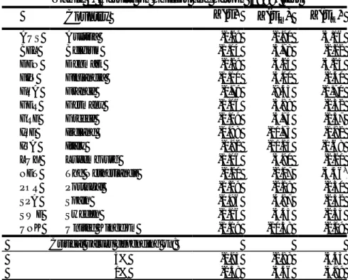
Table 3. Results of estimation from monthly inflation rates on EU countries

d_k estimations * k d estimations 1 = m m=2 m=3 m=1 m=2 m=3 AUS 0.20 0.33 0.29 -0.44 -0.41 -0.48 BEL 0.16 0.20 0.12 -0.68 -0.63 -0.55 DEN 0.33 0.45 0.37 -0.55 -0.47 -0.47 FIN 0.29 0.33 0.23 -0.77 -0.60 -0.56 FRA 0.24 0.42 0.33 -0.40 -0.53 -0.52 GER 0.35 0.42 0.33 -0.49 -0.49 -0.50 GRE 0.31 0.57 0.46 -0.40 -0.56 -0.65 IRE 0.32 0.25 0.16 -0.44 -0.42 -0.41 ITA 0.41 0.58 0.49 -0.44 -0.33 -0.32 LUX 0.44 0.57 0.49 -0.47 -0.57 -0.50 NET 0.20 0.39 0.31 -0.52 -0.42 -0.50 POR 0.24 0.23 0.14 -0.41 -0.37 -0.28 SPA 0.27 0.33 0.18 -0.35 -0.48 -0.48 SWE 0.28 0.43 0.34 -0.40 -0.42 -0.39 UNK 0.16 0.35 0.27 -0.60 -0.67 -0.56 Standard error 0.150 0.110 0.096 0.150 0.110 0.096 Notes:

a) In all cases unit root hypothesis is rejected at 1% significance level.

b) Standard errors have been obtained over 10000 ARFIMA(0,1,0) series of 512 observations. Results obtained from ARFIMA(1,d,1) models with different autoregressive, moving average parameters are very close to those obtained from ARFIMA(0,1,0) models.

For all countries we find estimates significantly different from 1 as well as from 0. So from the results in Table 3, it is deduced that all estimations lead one to reject the null hypothesis that d_k* =0, that is, we reject the unit root hypotesis in inflation rates. Then we conclude the shocks on the inflation rates have only temporal effects that gradually diminish.

5. The order of integration of the interanual inflation rates.

Some of previous work about persistence of inflation are based on inteannual inflation rates, not in monthly inflation rates. The purpose of this section is to estimate the orders of integration of interannual inflation rates on EU countries and to compare with results obtained in previous section about monthly inflation rates.

We have calculated interannual inflation rates as Y_kt =(1−L12)logI_kt

and we have used the same method as in previous section to obtain results presented in Table 4. From these results it is deduced that the immense majority of estimations lead one to not reject the null hypothesis that * =0

k

d , that is to say, the rates of inflationX_kt are I(1).

Table 4. Results of estimation from interannual inflation rates on EU countries

d_k estimations * k d estimations 1 = m m=2 m=3 m=1 m=2 m=3 AUS 0.93 1.00 0.76 -0.17 0.05 0.12 BEL 0.83 0.88 0.81 0.01 0.01 -0.11 DEN 1.00 1.03 0.87 -0.12 -0.12 -0.03 FIN 0.87 0.84 0.81 -0.27 -0.09 0.06 FRA 0.97 0.99 0.76 0.06 0.16 0.22 GER 0.98 0.99 0.91 -0.10 0.07 0.04 GRE 1.09 1.08 0.81 0.03 0.08 0.13 IRE 0.91 0.92 0.90 0.09 0.18 0.22* ITA 1.05 1.05 0.96 0.11 0.18 0.27* LUX 1.05 1.08 0.98 -0.08 0.09 -0.05 NET 0.98 1.01 0.73 0.00 -0.03 0.14 POR 0.88 0.88 0.80 -0.22 -0.18 -0.01 SPA 0.86 0.82 0.75 0.04 -0.05 0.04 SWE 1.00 1.03 0.89 -0.28 -0.18 0.09 UNK 0.98 0.97 0.94 -0.12 0.12 0.21* Standard error 0.150 0.110 0.096 0.150 0.110 0.096 Notes:

a) (*) indicates unit root hypothesis is rejected at 5% significance level. In any case that hypothesis is rejected at 1% significance level.

b) Standard errors have been obtained over 10000 ARFIMA(0,1,0) series of 512 observations. Results obtained from ARFIMA(1,d,1) models with different autoregressive, moving average parameters are very close to those obtained from ARFIMA(0,1,0) models.

Only in the case of Ireland, Italy and the United Kingdom and only using 3

=

m , are estimations obtained that suggest that said rates of inflation can be integrated in an order slightly superior to the unit. Nevertheless, the fact that with

1 =

m and with m =2, X_kt ∼ I(1) can be rejected.

These seems a hard contradiction with previous results, but we think not. To understand that, it’s important to note that

kt kt

kt

kt L I L L L X S L X

Y =(1− 12)log =(1+ + 2 +...+ 11) = ( )

so interannual inflation rates can be shown as a filtered output of inflation rates,

t t S L X Y = ( ) , where ( ) (1 2 ... 11) L L L L

S = + + + . Note the S(L) filter have gain function 2 1 12 ) cos( 1 ) 12 cos( 1 1 1 ) ( ) (       − − = − − = = ω ω ω ω _ωω i i i e e e S G

with zeros at Fourier frequencies

12 2 j

j

π

ω = where s=1,..,6 (see Graph 1). Then )

(L

S is a non-invertible filter.

Graph 1. Gain function of S L( ) filter.

0 2 4 6 8 10 12 14 0.00 0.31 0.63 0.94 1.26 1.57 1.88 2.20 2.51 2.83 3.14

It’s well known that time domain unit root tests mustn’t be applied to non-invertible series because this tests are hardly biased5. So it’s important to analyse what is the effect of S(L) filter in estimators of fractional integration parameter.

To explore the behavior of WOLS estimator of fractional difference parameter when series are obtained using S(L) filter, we generated series of 100 observations from an ARFIMA(1,d,0) model, (1−L)d(1−φL)X_t =ε_t and we used the WOLS method to calculate estimations of d based on both X_t and

t

t S L X

Y = ( ) .

All the results presented in Annex 1 show we can’t use WOLS estimator with noninvertible series because it’s hardly biased. In other simulation results we have seen this problems are shared with other fractional integration parameter estimators as the Geweke and Porter-Hudak (1983) one. The most important conclussion of this results is persistence in inflation rates mustn’t be analysed using interannual inflation rates data.

6. Conclusions

As has been commented in the introduction, in spite of its importance not only for macroeconomic theory as for taking decisions for the political economy, there exists considerable controversy concerning the level of persistence of the rates of inflation. We understand by the term persistence to what extent future inflation is affected by the shocks that could have occurred in the former evolution of said variable.

In this paper the level of persistence of the rates of inflation in the EU has been analysed by using an extremely general and flexible model that allows the existence of fractional integration. Starting with said model, and through the use

of the theory of wavelets to obtain estimations of the order of integration, it has been confirmed that the empirical evidence allows reject the hypothesis that the rates of inflation in the EU countries have a unit root. Therefore, the shocks that can affect said rates of inflation for the present can’t be transmitted in a permanent way to future values of said inflation. Moreover, it’s shown that interannual inflatio rates data musn’t be used to analyse persistence due to the effect of non-invertible filters on inference about fractional integration parameter.

References

Agiakloglou, C.; P. Newbold and M. Wohar (1992): "Bias in an estimator of the fractional difference parameter", Journal of Time Series Analysis 14, 235-246. Barsky, R.B. (1987): "The Fisher hypothesis and the forecastability and persistence of inflation", Journal of Monetary Economics 19, 3-24.

Daubechies, I. (1988): "Orthonormal bases of compactly supported wavelets",

Communications on Pure and Applied Mathematics 41, 909-996.

Dickey, D.A. and W.A. Fuller (1981): "Likelihood ratio statistics for autoregressive time series with a unit root", Econometrica 49, 1057-1072.

Diebold, F.X. and G.D. Rudebusch (1989): "Long memory and persistence in aggregate output", Journal of Monetary Economics 24, 189-209.

Fuller, W.A. (1976): Introduction to statistical time series. John Wiley and Sons, New York.

Geweke, J. and S. Porter-Hudak (1983): "The estimation and application of long memory time series models", Journal of Time Series Analysis 4, 221-238.

Ghysels, E. and P. Perron (1993): "The effect of seasonal adjustment filters on tests for a unit root", Journal of Econometrics 55, 57-98.

Gradshteyn, I.S. and Ryzhik, I.M. (1965): Tables of Integrals, Series and

Hassler U. and J. Wolters (1995): "Long memory in inflation rates: international evidence", Journal of Business and Economic Statistics 13, 37-45.

Heil, C. and D. Walnut (1989): "Continuous and discrete wavelet transforms",

SIAM Review 31, 628-666.

Hurvich, C.M.; R. Deo and J. Brodsky (1998): "The mean squared error of Geweke and Porter-Hudak’s estimator of the memory parameter of a long-memory time series", Journal of Time Series Analysis 19, 19-46.

Jensen, M.J. (1999): "Using wavelets to obtain a consistent ordinary least squares estimator of the long-memory parameter", Journal of Forecasting 18, 17-32. Kirchgässner, G. and J. Wolters (1993): "Are real interest rates stable? An international comparison", in Studies in Applied Econometrics, eds. H. Schneeweiss y K.F. Zimmermann. Heidelberg, Physica-Verlag, pp. 214-238. MacDonald, R. and P.D. Murphy (1989): "Testing for the long run relationship between nominal interest rates and inflation using cointegration techniques",

Applied Economics 21, 439-447.

Phillips, P.C.B. and P. Perron (1988): "Testing for a unit root in time series regression", Biometrika 75, 335-346.

Porter-Hudak, S. (1990): "An application of the seasonal fractionally differenced model to the monetary aggregates", Journal of the American Statistical

Association 18, 502-527.

Press, W.H.; Flannery, B.P.; Teukolsky, S.A and W.T. Vetterling (1992):

Numerical recipes: the art of scientific computing. Cambridge University Press,

Cambridge.

Smith, J.; N. Taylor and S. Yadaf (1997): "Comparing the bias and misspecification in ARFIMA models", Journal of Time Series Analysis 18, 502-527.

Sowell, F. (1990): "The fractional root distribution", Econometrica 58, 495-505. Wickens, M. and E. Tzavalis (1992): "Forecasting inflation from the term structure: a cointegration approach", Discussion Paper 13-92. Center of Economic Forecasting, London Business School.

Annex 1. Monte Carlo results.

To explore the behavior of the WOLS estimator of fractional difference parameter when filter S(L) is applied, we generated series of 100 observations from an ARFIMA(1,d,0) model, d _{t t}

X L

L −φ =ε

− ) (1 ) 1

( , and we used the WOLS

method to calculate estimations of d on X_t and Y_t = S(L)X_t. The data are generated according to Hoskink (1984) and we have computed mean, standard deviation and mean squared error of WOLS estimations for different values of

dand φ. Simulations are reported for two sample sizes, the first containing 256 observations and the second 512. Most important results are presented in following tables.

Table A1. Mean of estimations of fractional integration parameter when φ=0 and T=256. Estimation from X_t Estimation from Y_t

d m=1 m=2 m=3 m=1 m=2 m=3 -0.45 -0.46 -0.40 -0.36 0.13 0.30 0.44 -0.35 -0.41 -0.34 -0.29 0.23 0.38 0.52 -0.25 -0.33 -0.27 -0.22 0.30 0.47 0.61 -0.15 -0.23 -0.20 -0.16 0.38 0.54 0.68 -0.05 -0.13 -0.10 -0.08 0.46 0.62 0.76 0.05 -0.02 0.01 0.03 0.53 0.70 0.83 0.15 0.09 0.12 0.13 0.61 0.76 0.90 0.25 0.19 0.22 0.24 0.67 0.84 0.97 0.35 0.30 0.32 0.33 0.76 0.90 1.03 0.45 0.42 0.43 0.44 0.83 0.97 1.10

Table A2. Mean of estimations of fractional integration parameter when φ=0 and T=512. Estimation from X_t Estimation from Y_t

d m=1 m=2 m=3 m=1 m=2 m=3 -0.45 -0.46 -0.39 -0.35 0.08 0.22 0.35 -0.35 -0.39 -0.33 -0.29 0.15 0.29 0.43 -0.25 -0.32 -0.27 -0.23 0.23 0.37 0.51 -0.15 -0.24 -0.18 -0.15 0.30 0.45 0.58 -0.05 -0.14 -0.10 -0.08 0.37 0.51 0.66 0.05 -0.06 -0.01 0.01 0.46 0.60 0.74 0.15 0.04 0.10 0.12 0.54 0.67 0.81 0.25 0.14 0.21 0.23 0.62 0.75 0.87 0.35 0.24 0.31 0.34 0.70 0.82 0.94 0.45 0.35 0.42 0.44 0.77 0.89 1.00

Table A3. Mean of estimations of fractional integration parameter when φ=0 5. and T=256. Estimation from X_t Estimation from Y_t

d m=1 m=2 m=3 m=1 m=2 m=3 -0.45 -0.27 -0.17 -0.09 0.31 0.51 0.71 -0.35 -0.20 -0.10 -0.01 0.37 0.57 0.77 -0.25 -0.12 -0.02 0.07 0.45 0.64 0.93 -0.15 -0.06 0.05 0.14 0.52 0.72 0.89 -0.05 0.03 0.13 0.22 0.57 0.78 0.96 0.05 0.11 0.21 0.30 0.64 0.83 1.01 0.15 0.19 0.30 0.38 0.71 0.88 1.05 0.25 0.30 0.39 0.47 0.75 0.93 1.10 0.35 0.38 0.47 0.54 0.83 0.99 1.14 0.45 0.49 0.57 0.63 0.89 1.04 1.19

Table A4. Mean of estimations of fractional integration parameter when φ=0 5. and T=512. Estimation from X_t Estimation from Y_t

d m=1 m=2 m=3 m=1 m=2 m=3 -0.45 -0.29 -0.20 -0.13 0.20 0.38 0.55 -0.35 -0.22 -0.13 -0.06 0.28 0.45 0.62 -0.25 -0.14 -0.06 0.02 0.34 0.51 0.69 -0.15 -0.06 0.02 0.10 0.41 0.58 0.75 -0.05 0.02 0.11 0.17 0.48 0.64 0.81 0.05 0.11 0.19 0.25 0.55 0.71 0.87 0.15 0.20 0.27 0.34 0.62 0.76 0.92 0.25 0.30 0.37 0.43 0.69 0.83 0.98 0.35 0.39 0.45 0.51 0.75 0.89 1.03 0.45 0.50 0.56 0.60 0.82 0.95 1.07

Table A5. Mean of estimations of fractional integration parameter when φ=0 9. and T=256. Estimation from X_t Estimation from Y_t

d m=1 m=2 m=3 m=1 m=2 m=3 -0.45 0.14 0.26 0.33 0.64 0.87 1.05 -0.35 0.22 0.34 0.41 0.71 0.92 1.10 -0.25 0.30 0.42 0.50 0.73 0.95 1.13 -0.15 0.37 0.49 0.57 0.79 1.00 1.18 -0.05 0.45 0.58 0.66 0.83 1.03 1.20 0.05 0.53 0.66 0.74 0.88 1.07 1.22 0.15 0.60 0.73 0.81 0.91 1.11 1.26 0.25 0.70 0.81 0.91 0.94 1.13 1.28 0.35 0.76 0.89 0.98 1.01 1.17 1.30 0.45 0.84 0.96 1.05 1.06 1.19 1.32

Table A6. Mean of estimations of fractional integration parameter when φ=0 9. and T=512. Estimation from X_t Estimation from Y_t

d m=1 m=2 m=3 m=1 m=2 m=3 -0.45 0.08 0.20 0.30 0.51 0.71 0.90 -0.35 0.16 0.28 0.37 0.56 0.76 0.94 -0.25 0.25 0.37 0.46 0.62 0.81 1.00 -0.15 0.32 0.45 0.54 0.66 0.86 1.03 -0.05 0.41 0.52 0.62 0.72 0.91 1.07 0.05 0.49 0.60 0.70 0.78 0.95 1.11 0.15 0.57 0.68 0.78 0.83 0.99 1.14 0.25 0.67 0.77 0.86 0.89 1.03 1.18 0.35 0.73 0.84 0.94 0.93 1.08 1.21 0.45 0.83 0.93 1.01 0.99 1.12 1.24

Table A7. Standard deviation when φ=0 and T=256. Estimation from X_t Estimation from Y_t

d m=1 m=2 m=3 m=1 m=2 m=3 -0.45 0.180 0.151 0.130 0.201 0.147 0.132 -0.35 0.191 0.148 0.125 0.191 0.142 0.123 -0.25 0.194 0.153 0.126 0.185 0.139 0.124 -0.15 0.190 0.153 0.126 0.186 0.143 0.126 -0.05 0.189 0.153 0.129 0.178 0.149 0.119 0.05 0.186 0.159 0.128 0.185 0.143 0.130 0.15 0.197 0.147 0.128 0.183 0.142 0.124 0.25 0.182 0.143 0.129 0.194 0.140 0.122 0.35 0.188 0.146 0.124 0.184 0.146 0.125 0.45 0.180 0.141 0.123 0.187 0.138 0.116

Table A8. Standard deviation when φ=0 and T=512. Estimation from X_t Estimation from Y_t

d m=1 m=2 m=3 m=1 m=2 m=3 -0.45 0.154 0.115 0.090 0.141 0.109 0.093 -0.35 0.153 0.112 0.088 0.143 0.111 0.091 -0.25 0.152 0.111 0.090 0.145 0.112 0.090 -0.15 0.151 0.112 0.092 0.152 0.108 0.089 -0.05 0.147 0.115 0.093 0.151 0.115 0.092 0.05 0.146 0.110 0.090 0.149 0.111 0.092 0.15 0.145 0.110 0.091 0.152 0.105 0.091 0.25 0.144 0.109 0.093 0.147 0.111 0.087 0.35 0.142 0.109 0.096 0.156 0.110 0.089 0.45 0.140 0.106 0.090 0.154 0.114 0.090

Table A9. Standard deviation when φ=0 5. and T=256. Estimation from X_t Estimation from Y_t

d m=1 m=2 m=3 m=1 m=2 m=3 -0.45 0.190 0.141 0.126 0.193 0.145 0.117 -0.35 0.180 0.143 0.124 0.192 0.147 0.117 -0.25 0.182 0.147 0.123 0.183 0.140 0.121 -0.15 0.194 0.156 0.125 0.188 0.133 0.119 -0.05 0.195 0.154 0.126 0.187 0.134 0.114 0.05 0.190 0.151 0.126 0.183 0.138 0.112 0.15 0.188 0.144 0.128 0.192 0.145 0.109 0.25 0.179 0.142 0.127 0.199 0.146 0.110 0.35 0.186 0.143 0.124 0.181 0.135 0.112 0.45 0.183 0.140 0.123 0.186 0.138 0.105

Table A10. Standard deviation when φ=0 5. and T=512. Estimation from X_t Estimation from Y_t

d m=1 m=2 m=3 m=1 m=2 m=3 -0.45 0.155 0.111 0.093 0.154 0.110 0.096 -0.35 0.152 0.109 0.088 0.147 0.112 0.087 -0.25 0.154 0.115 0.087 0.149 0.110 0.087 -0.15 0.147 0.112 0.090 0.148 0.113 0.089 -0.05 0.154 0.111 0.092 0.139 0.109 0.091 0.05 0.150 0.111 0.092 0.153 0.111 0.086 0.15 0.144 0.110 0.092 0.152 0.113 0.087 0.25 0.151 0.109 0.089 0.150 0.110 0.088 0.35 0.144 0.114 0.094 0.150 0.115 0.091 0.45 0.145 0.109 0.091 0.159 0.118 0.092

Table A11. Standard deviation when φ=0 9. and T=256. Estimation from X_t Estimation from Y_t

d m=1 m=2 m=3 m=1 m=2 m=3 -0.45 0.126 0.138 0.124 0.186 0.135 0.111 -0.35 0.124 0.140 0.126 0.179 0.145 0.110 -0.25 0.123 0.143 0.129 0.189 0.130 0.112 -0.15 0.125 0.146 0.132 0.180 0.134 0.101 -0.05 0.126 0.148 0.127 0.185 0.142 0.108 0.05 0.124 0.143 0.129 0.182 0.133 0.105 0.15 0.128 0.146 0.133 0.199 0.135 0.106 0.25 0.130 0.141 0.123 0.195 0.137 0.102 0.35 0.120 0.142 0.123 0.179 0.128 0.109 0.45 0.128 0.144 0.123 0.177 0.133 0.102

Table A12. Standard deviation when φ=0 9. and T=512. Estimation from X_t Estimation from Y_t

d m=1 m=2 m=3 m=1 m=2 m=3 -0.45 0.145 0.109 0.093 0.151 0.108 0.086 -0.35 0.144 0.118 0.089 0.146 0.109 0.087 -0.25 0.144 0.109 0.086 0.150 0.111 0.089 -0.15 0.144 0.105 0.093 0.151 0.112 0.083 -0.05 0.142 0.111 0.089 0.147 0.106 0.085 0.05 0.153 0.107 0.092 0.151 0.106 0.081 0.15 0.141 0.110 0.095 0.149 0.110 0.082 0.25 0.146 0.107 0.090 0.142 0.110 0.084 0.35 0.152 0.110 0.094 0.148 0.107 0.086 0.45 0.144 0.111 0.092 0.144 0.108 0.082

Table A13. Mean squared error when φ=0 and T=256. Estimation from X_t Estimation from Y_t

d m=1 m=2 m=3 m=1 m=2 m=3 -0.45 0.032 0.025 0.025 0.377 0.581 0.808 -0.35 0.040 0.022 0.019 0.375 0.557 0.777 -0.25 0.044 0.024 0.016 0.340 0.541 0.750 -0.15 0.043 0.026 0.016 0.312 0.500 0.700 -0.05 0.042 0.026 0.018 0.291 0.466 0.675 0.05 0.040 0.027 0.017 0.266 0.438 0.620 0.15 0.043 0.022 0.017 0.247 0.391 0.584 0.25 0.037 0.021 0.017 0.211 0.364 0.532 0.35 0.038 0.022 0.016 0.200 0.326 0.473 0.45 0.033 0.021 0.015 0.182 0.288 0.432

Table A14. Mean squared error when φ=0 and T=512. Estimation from X_t Estimation from Y_t

d m=1 m=2 m=3 m=1 m=2 m=3 -0.45 0.024 0.017 0.018 0.296 0.462 0.646 -0.35 0.025 0.013 0.011 0.269 0.423 0.611 -0.25 0.028 0.013 0.008 0.247 0.393 0.580 -0.15 0.031 0.014 0.008 0.225 0.372 0.542 -0.05 0.031 0.016 0.009 0.196 0.328 0.507 0.05 0.032 0.016 0.010 0.194 0.319 0.479 0.15 0.033 0.015 0.009 0.176 0.285 0.437 0.25 0.032 0.013 0.009 0.162 0.262 0.397 0.35 0.033 0.014 0.009 0.143 0.238 0.356 0.45 0.029 0.012 0.008 0.129 0.204 0.311

Table A15. Mean squared error when φ=0 5. and T=256. Estimation from X_t Estimation from Y_t

d m=1 m=2 m=3 m=1 m=2 m=3 -0.45 0.069 0.100 0.148 0.611 0.950 1.361 -0.35 0.055 0.082 0.134 0.553 0.867 1.271 -0.25 0.051 0.075 0.118 0.528 0.818 1.189 -0.15 0.046 0.063 0.101 0.486 0.773 1.102 -0.05 0.044 0.057 0.090 0.425 0.700 1.025 0.05 0.040 0.050 0.080 0.385 0.625 0.933 0.15 0.037 0.043 0.067 0.346 0.552 0.828 0.25 0.035 0.039 0.063 0.285 0.484 0.730 0.35 0.036 0.036 0.052 0.261 0.432 0.638 0.45 0.035 0.033 0.047 0.229 0.365 0.552

Table A16. Mean squared error when φ=0 5. and T=512. Estimation from X_t Estimation from Y_t

d m=1 m=2 m=3 m=1 m=2 m=3 -0.45 0.048 0.074 0.112 0.450 0.706 1.012 -0.35 0.039 0.061 0.094 0.419 0.647 0.949 -0.25 0.036 0.050 0.080 0.376 0.597 0.897 -0.15 0.029 0.043 0.071 0.338 0.547 0.825 -0.05 0.029 0.036 0.057 0.298 0.489 0.742 0.05 0.027 0.032 0.049 0.277 0.446 0.679 0.15 0.023 0.028 0.046 0.243 0.389 0.597 0.25 0.026 0.025 0.040 0.218 0.351 0.533 0.35 0.022 0.024 0.035 0.185 0.309 0.466 0.45 0.023 0.024 0.031 0.163 0.260 0.392

Table A17. Mean squared error when φ=0 9. and T=256. Estimation from X_t Estimation from Y_t

d m=1 m=2 m=3 m=1 m=2 m=3 -0.45 0.368 0.528 0.617 1.233 1.749 2.260 -0.35 0.344 0.494 0.595 1.148 1.626 2.102 -0.25 0.319 0.468 0.580 1.004 1.466 1.930 -0.15 0.288 0.436 0.539 0.913 1.339 1.766 -0.05 0.269 0.416 0.520 0.802 1.189 1.569 0.05 0.249 0.391 0.491 0.729 1.052 1.385 0.15 0.220 0.361 0.459 0.622 0.937 1.238 0.25 0.216 0.339 0.448 0.520 0.785 1.072 0.35 0.182 0.312 0.411 0.472 0.685 0.910 0.45 0.167 0.284 0.381 0.404 0.572 0.761

Table A18. Mean squared error when φ=0 9. and T=512. Estimation from X_t Estimation from Y_t

d m=1 m=2 m=3 m=1 m=2 m=3 -0.45 0.307 0.438 0.564 0.940 1.356 1.818 -0.35 0.279 0.411 0.532 0.857 1.248 1.684 -0.25 0.267 0.390 0.511 0.773 1.144 1.562 -0.15 0.241 0.366 0.488 0.683 1.028 1.409 -0.05 0.232 0.341 0.455 0.614 0.926 1.268 0.05 0.216 0.319 0.430 0.553 0.818 1.126 0.15 0.197 0.295 0.406 0.482 0.716 0.987 0.25 0.195 0.279 0.380 0.430 0.627 0.872 0.35 0.170 0.256 0.353 0.360 0.539 0.740 0.45 0.163 0.243 0.323 0.310 0.463 0.629