UNIVERSITY OF MACERATA
DEPARTIMENT OF ECONOMICS AND LAW
PhD Programme in
QUANTITATIVE METHODS FOR POLICY EVALUATION
Curriculum
MULTISECTORAL AND COMPUTATIONAL METHODS OF ANALYSIS FOR ECONOMIC POLICY
XXXIII cycle
Environment, equality, and resilience: fiscal policy assessed
through General Equilibrium Models
SUPERVISOR CANDIDATE
Prof. Claudio Socci Silvia D’Andrea
COORDINATOR
Prof. Luca De Benedictis
1 INDEX
INDEX ... 1
INDEX OF TABLES AND FIGURES... 3
A renewed debate on fiscal policy effectiveness ... 5
References ... 12
CHAPTER 1 - INEQUALITY AND FLAT INCOME TAX IN ITALY ... 13
1.1. Can flat tax stimulate growth and reduce inequality? ... 13
1.2. How the application of flat tax is modelled ... 19
1.2.1. The Households breakdown into income deciles ... 19
1.2.2. A static CGE model to evaluate the economic impact ... 24
1.3. Income tax reform: implementation and results ... 31
1.4. Concluding: no trade-off between growth and equality ... 40
References for Chapter 1 ... 43
Appendix 1. ISTAT National Accounts – Classification of activities and products ... 45
Appendix 2. Parameters, variables and equations of the static model ... 47
Appendix 3 - Sensitivity analysis – Chapter 1 ... 51
CHAPTER 2 – ECONOMIC GROWTH AND A U.S. FEDERAL CARBON TAX... 53
2.1. Environment should be at the core of public policy ... 53
2.2. Construction of the Framework ... 56
2.2.1. National Accounts and environmental data ... 56
2.2.2. A dynamic CGE model for the U.S. economic system ... 60
2.3. Income taxes reform coupled with the carbon tax introduction ... 67
2.3.1. - Simulation 1: Corporate income tax reduction ... 69
2.3.2. - Simulation 2: Household income tax reduction ... 72
2.3.3. - Simulation 3: Household income tax reduction and public expenditure reduction ... 74
2.3.4. - Simulation 4: Household income tax reduction and the introduction of a carbon tax ... 75
2.4. Concluding: Carbon tax does not appear harmful ... 77
References for Chapter 2 ... 81
Appendix 4. BEA - Products and Industries Classifications ... 85
Appendix 5: Parameters, variables and equations of the dynamic model ... 87
Appendix 6. Employment percent change – simulation 4 ... 92
Appendix 7. Sensitivity analysis – Chapter 2 ... 93
CHAPTER 3 - SUPPORTS TO FIRMS’ LIQUIDITY ... 94
2
3.2. A dynamic CGE Model integrated with financial instruments ... 99
3.3. Estimation of the liquidity position of firms... 109
3.4. Government measures in support of businesses liquidity ... 119
3.5. The effects of supports at macroeconomic level ... 122
3.6. Results applied to ORBIS data... 127
3.7. Concluding: The better strategy for the short-term is a long period programme ... 133
References for Chapter 3 ... 135
Appendix 8: Real and Financial Products in the FSAM ... 138
Appendix 9: Parameters, variables and equations of the dynamic model ... 140
Appendix 10. Sensitivity analysis – Chapter 3 ... 146
INDEX OF TABLES Table 1 - Propensity Score Matching results and statistics ... 21
Table 2 – Number of Households’ per income decile before and after matching ... 22
Table 3 – Percentage of Households’ per income decile before and after matching ... 23
Table 4 – The structure of interactions among agents (a) ... 26
Table 5 – Structure of the actual income tax in Italy (a) ... 32
Table 6 - Flat Tax simulations main effects (percent change from benchmark) ... 35
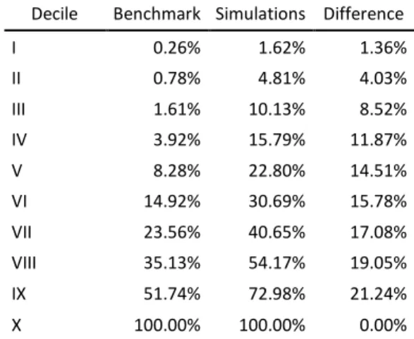
Table 7 - Income tax distribution (cumulative percentages) ... 39
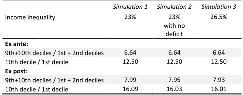
Table 8 - Income inequality ... 40
Table 9: Sensitivity analysis on σv - Effects on macroeconomic aggregates ... 51
Table 10: Sensitivity analysis on Sigma utility - Effects on macroeconomic aggregates ... 52
Table 11. The Social Accounting Matrix and the structure of interactions among agents (a) ... 58
Table 12. Impact of the reduction of the corporate tax on income ... 70
Table 13. Impact of the reduction of the households’ income tax ... 72
Table 14. Impact of the reduction of the households’ income tax with provision through public expenditure reduction (percentage change from benchmark, in real terms) ... 74
Table 14. Impact of the reduction of the households’ income tax with provision through a Federal carbon tax (percentage change from benchmark, in real terms) ... 76
Table 16. Simulation 4 - sensitivity analysis (percentage change from benchmark, in real terms) ... 93
Table 17 - The structure of interactions among agents (a) ... 101
Table 18 — Distribution of macroeconomic variables by firm class ... 117
Table 19 — Distribution of firms by industry and size class ... 118
Table 20 – Percentage of liquidity constrained firms by firm class in case of a -20% turnover ... 119
Table 21 - Temporary reduction of employers’ social security contribution by 1 percent of GDP ... 123
Table 22 - Raise in State guarantees to bank loans by 1 percent of GDP ... 124
Table 23 – One-off contribution to capital cost of firms by 1 percent of GDP... 125
Table 24 – Emission of Treasury Bonds by 1 percent of GDP ... 126
Table 25 – ECB purchase of Treasury Bonds by 1 percent of GDP ... 127
3
Table 24 – Sensitivity analysis- Temporary reduction of employers’ social security contribution ... 146
Table 25 – Sensitivity analysis - Raise in State guarantees to bank loans by 1 percent of GDP... 147
INDEX OF FIGURES Figure 1 - Density function for treated and not treated before and after matching ... 22
Figure 2 – Income Circular Flow ... 25
Figure 3. Production function by industry and by commodity. ... 27
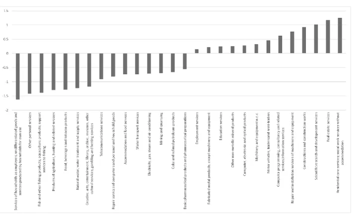
Figure 4 – Scenario 1 – 23% in deficit - Products most affected after flat tax introduction ... 37
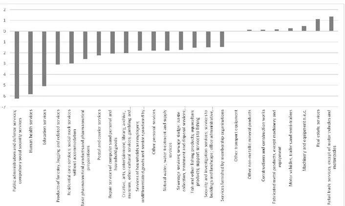
Figure 5 – Scenario 2 – 23% with provision - Products most affected after flat tax introduction ... 38
Figure 6 – Scenario 2 – 26.5% - Products most affected after flat tax introduction ... 38
Figure 7. Production function by industry and by commodity. ... 62
Figure 8. Greenhouse gas emissions - Impact of the reduction of the corporate tax on income ... 71
Figure 9. Greenhouse gas emissions - Impact of the reduction of the household tax on income ... 73
Figure 10. Greenhouse gas emissions: Impact of the reduction of the household tax on income, financed by public ... 75
Figure 11. Greenhouse gases emissions - Contribution of most relevant sectors (Percent changes compared to benchmark)... 77
Figure 12 – Scheme of the Dynamic Computable General Equilibrium Model with Financial Flows .... 102
Figure 13 - Production function by commodity ... 103
Figure 14 – short term liabilities on the sum of long term liabilities and net worth by industry ... 113
Figure 15 - short term, long term liabilities and net worth on turnover by industry ... 113
Figure 16 – industry size by number of persons employed ... 114
Figure 17 – Liquidity contraction carried by a 20% turnover contraction ... 116
Figure 18 – Effects on output of Government support measures ... 128
Figure 19 - trend in turnover and output in historical series ... 129
Figure 20 — Change in turnover and output by industry in historical series ... 130
4
Acknowledgements:
This thesis is dedicated to my husband, Gian Carlo. I would also like to thank:
My supervisor, Prof. Claudio Socci, for his patience while waiting for me to apply his lessons. Francesca Severini, Rosita Pretaroli and Giancarlo Infantino, for their precious hints and teachings. Stefano Deriu, an invaluable colleague, and a friend to overcome the difficulties encountered in my studies.
Ebano Maria Rita, Francesca Policastro and Lavinia Rotili, for their constant support and encouragement.
5 A renewed debate on fiscal policy effectiveness
With the financial crisis of 2007 and the COVID-19 epidemic crisis today, the debate on
the effectiveness of fiscal policy has been renewed, for which there remains a wide range of views
on the strength of macroeconomic effects, the channels through which these effects operate and the different effectiveness on the basis of a country’s starting economic conditions.
Some economists believe that it would be better to let fiscal policy have a countercyclical
impact only through automatic stabilisers and that discretionary fiscal policies are left to long-term
action, leading to less frequent changes. This is because discretionary fiscal policies are considered
not to have contributed to economic stability but rather to have destabilising effects (Taylor, 2000,
2009; Feldstein, 2002). However, the previous crises, in the 80s and 90s, were mainly supply-side
crises as a result of oil shocks, while the most recent crises have led to significant demand-side
effects, with increased restrictions on the availability of credit to households and firms, in an
environment of very low interest rates in which the effects of conventional monetary policy are
limited. It is clear that different conditions can lead to a different view on the effectiveness of fiscal
policies and the different role they can play in normal or crisis times. In particular, the role of automatic stabilisers is considered to play an essential role in ‘normal’ economic situations, while their usefulness has been judged to be low during severe recessions (Banca d’Italia, 2011).
By reviewing the literature, Hamming R., Kell M., Mahfouz S. (2002) highlight that the
appropriate fiscal policy response to an economic downturn depends on a number of factors, and
only a country-by-country approach by type of problem can find the best instrument. In particular,
several elements need to be considered: fiscal policy is more effective if the shock originates on
the demand side; the response of prices, interest rates and exchange rates may make it necessary
to assess whether fiscal policy should be accompanied by monetary policy; the influence on risk
premia of the duration of fiscal expansion and the sustainability of public debt should also be
6
associated with larger fiscal multipliers than tax cuts. Moreover, expenditure and fiscal measures
that have supply-side effects may have short-term impacts affecting expectations. Finally, the
behaviour of firms and households in saving and investment decisions is influenced by factors
such as liquidity constraints, expectations formation and confidence which are likely to be affected
by tax policy. The choice and timing of a tax policy is also influenced by the structure and the tax
burden, which have a different impact and different effects on economic activity according to the
country in which they are applied and the starting circumstances (Roeger W., In 't Veld J., 2009).
Recent findings of the European Commission (2020) show that the success of a policy lies
in a number of factors. The reforms that form part of an integrated package of measures seem to
be more effective, both because an appropriate sequencing of reforms and their coordination in
time is crucial, and because short-term forms of compensation included in the ‘package’ of
measures can make some reforms more acceptable. Not least, an evidence-based policy design,
leading to a coherent and comprehensive strategy, can facilitate the acceptance of a reform and,
therefore, the implementation of the reform itself.
Being taxation one of the most important tools of fiscal policies, the relationship between
taxation and economic growth represents a strongly debated question for researchers and policy
makers (Baxter M., King R. G. 1993).
Economic theory argues that taxes create distortions that negatively affect growth and
economic operators. According to the OECD1, corporate and personal income taxes have the
greatest negative impact on growth, while types of taxation on consumption, environment and
property are less harmful.
In a situation such as the present one, characterized by credit constraints, low interest rates
and deflationary shocks, Roeger W. and In’t Veld J. (2009) using a DSGE model have shown that
1 OECD, Going for Growth 2009
7
temporary fiscal policy ‘shocks’ can be more effective than in the past, but have significant effects in the case of expenditure interventions rather than on the tax reduction side.
These evidences, derived from the extensive literature on tax policy, do not take into
account the fact that tax policies now have to pursue a number of policy objectives, focusing not
only on economic growth but also on redistribution of income, resource allocation and environmental objectives. It was only since 2017 that, in its publication ‘Going for Growth’, the OECD has included the reduction of inequality as one of the political priorities that Governments
must also pursue. While the environment has long been one of the most controversial topics of
political debates, it has emerged as a global priority, especially with the latest crises, following
which the European Union has launched the Green New Deal and each Member State has adopted
its own Climate Plan2. It seems that there is also a stronger focus on environmental issues in the
USA and, although not at federal level, individual States have implemented a number of targets
ranging from energy efficiency to specific greenhouse gas reduction targets.
Tax policy instruments should also aim to improve the allocation of capital and labour
between firms and encourage firms to invest and innovate. Reforms in this field also include reforms to facilitate firms’ access to markets, including capital markets. A better allocation of resources increases the resilience of an industry, understood as the ability to cope with traumatic
events by adapting and overcoming them, such as a bamboo barrel, which falls under strong winds
without breaking.
Taking into account the previous issues, the present work deals with these three main goals:
equity, environment and resilience, analysing the instruments that have frequently emerged in the
recent policy debate to provide a different view on the effects of the instruments themselves. The
analysis is carried out though General Equilibrium Models.
8
The 2007 financial crisis and the actual pandemic crisis originated from different sources:
a lack of regulation that caused the liquidity shortages, in one case, and a lockdown that curbed
production and consumption, on the other. Nevertheless, what the 2007 crises have taught is that
to ensure the success of the reform effort it is necessary that policy instruments be constantly
updated to meet the new challenges, and that greater policy analysis be promoted to ensure that
the instruments implemented by Governments takes account of the specific circumstances faced
by a Country. This require an approach that is general and disaggregated. General Equilibrium
models in this context are widely applied because they are able to analyse economic effects from
different angles (Carrasco et al., 2013).
The first chapter deals with the introduction of flat tax in Italy. The political debate within
several developed and developing countries questioned over the profitability of introducing a “flat-tax” on households’ income to reduce the tax burden, simplify the tax system and boost the economic growth. The main concern is related to the direct, indirect and induced income
redistribution effect that could be generated by the reform of the tax system and thus generate a
final impact on income below the forecasts. In this perspective, this study provides a quantification
of how the introduction of the flat rate tax on income in Italy could affect the Italian economic
system. From the analysis of the theoretical and applied contributions that the literature provides,
it is not easy to draw a clear conclusion on the overall effect of a flat-tax system. Above all, it is
not so straightforward to determine whether the benefits offset any unwanted effects. In this perspective, this study aims to analyse the economic impact of the tax rates’ reform in Italy, assuming the introduction of a unique tax rate on household income, replacing the present
progressive taxation on personal income. The main purpose of the analysis is evaluating the impact
of a tax reform considering all the effects that could be generated within the income circular flow
moving to a flat tax system. The aim is to contribute to the debate on the flat tax profitability by
9
analysis is carried out through the Italian Social Accounting Matrix for 2016 built for the purpose,
where the Households Institutional Sector is broken down by income deciles. The MAC18
Computable General Equilibrium (CGE) model developed by the Department of Economics and
Law of the University of Macerata is then calibrated according to the new SAM. The CGE model
allows providing a realistic and coherent picture of the income circular flow in Italy and allows
assessing the direct, indirect, and induced effects of the reform on both macroeconomic variables
and income distribution. By this way, the opposite results emerging from the literature can be
addressed, as well as the main features and effects of a flat tax in Italy can be highlighted. Countries
experiences, indeed, are very different not only for the different choices in terms of flat tax
adopted, but also in terms of starting point conditions, which are essential in determining the
effects on growth, State revenue and inequality. Three policy scenarios are analysed assuming
different tax rates and different hypothesis on the policy funding by the Government. No
simulation shows a trade-off between growth and inequality, while a negative effect on real GDP
occurs, coupled with an uneven effect on Households disposable income.
In the second chapter, to take into account the increasing concern for climate change, the
introduction of a carbon tax on productive activities in the USA at the Federal level is envisaged.
The study demonstrates that fiscal reforms can be combined with environmental measures, to
achieve the complex target represented by economic growth and environmental protection. In this
vein, this study evaluates the economic and environmental impact of the reorganisation of federal
taxation on corporate and personal income occurred in USA, coupled with the introduction of a
carbon tax on economic activities. The analysis is carried out through a dynamic CGE model
calibrated on a U.S. Social Accounting Matrix (SAM) with environmental accounts. The U.S.
SAM for 2017 has been built for the purpose, by also integrated it with environmental data, by
using the Environmental Protection Agency data on greenhouse gas emissions allocated to
10
activity, so to look also at the effects on employment of the fiscal policy proposed in the paper. A
dynamic Computable General Equilibrium (CGE) model has been constructed, calibrated on the
U.S. (SAM) for 2017, in order to analyse the effects during time. The work demonstrate that the
carbon tax can have a twofold objective. On the one side, the carbon tax can relieve the loss of
federal revenue following the personal income tax reduction. On the other side, the greenhouse
gas tax is not detrimental for growth, on the contrary it may constitute a tax dividend useful to
pursue other objectives not only for the environment, but also for health, work and fair taxation.
Results indicate that the reduction of personal income tax is more geared to economic growth
compared to the reduction of corporate income tax. Moreover, if the personal income tax reduction
is financed with the introduction of a carbon tax on economic activities, there is no harm to the
economic growth and a benefit for the environment arises.
Finally, the third chapter aims at assessing the impact of the policies put in place by the
Government to support businesses during crises times so to reduce liquidity constraints and
increasing resilience. The approach is twofold: in a first phase, through a general economic
equilibrium model the economic impacts of a shock can be assessed, without excluding the effects
on other sectors of the economy (Verikios, 2016 e 2020). Unlike previous works, the effectiveness
of the policies implemented by the government and which are likely to improve the liquidity of
businesses is assessed through a financial dynamic CGE model, able to capture also the changes
in financial assets and liabilities of the Institutional Sectors. Two policies are considered: firstly,
the reduction in employers’ social security contributions, aimed at reducing the tax wedge, which
has an impact on the economic account component of liquidity. Secondly, the increase in State
guarantees granted through the Guarantee Fund for SMEs, which are intended to make it easier to
obtain credit and, therefore, to affect the liquidity component linked to bank credit.
The second phase of the work involves the integration of CGE model with the main
business data, taken from the ORBIS database, so to have the possibility to assess how the sectoral
11
are larger, the more industries are resilient to exogenous shocks that, translating into lower
revenues, put pressure on liquidity and solvency. Considering the results from the point of view of
the opportunity of implementing a policy, it emerges that some sectors would benefit more from
the tax wedge reduction, while others from the increase in State guarantees, depending on the
structure of the sector itself. Thus, it would be appropriate to implement policies at sectoral level,
12 References
Banca d’Italia (2011), Fiscal Policy – lessons from the crisis. Papers presented at the Banca d’Italia workshop held in Perugia, 25-27 March, 2010 in: Seminari e Convegni No.6 Febbraio 2011.
European Commission (2020), Understanding the political economy of reforms: evidence from the EU – Technical Note for the Eurogroup https://www.consilium.europa.eu/media/45511/ares-2020-4586969_eurogroup-note-on-political-economy-of-reforms.pdf
Feldstein, M. (2002), The Role for Discretionary Fiscal Policy in a Low Interest Rate Environment, NBER Working Paper No. W9203.
IMF (2016), World Economic Outlook – Chap.3 Time for A Supply-Side Boost? Macroeconomic Effects of Labour and Product Market Reforms in Advanced Economies.
Hamming R., Kell M., Mahfouz S. (2002), The effectiveness of fiscal policy in stimulating economic activity – a review of the literature, IMF Working Paper WP/02/208.
https://www.imf.org/external/pubs/ft/wp/2002/wp02208.pdf
Metelli L. and Pallara K. (2020), Fiscal space and the size of fiscal multiplier, Banca d’Italia – Temi di Discussione No.1293.
OECD (2008). Taxing Wages. 2006-2007.
OECD – Going for Growth, 2009 – 2017.
Roeger W., in 't Veld J. (2009), Fiscal Policy with Credit Constrained Households - European Commission, DG ECFIN - Economic and Financial Affairs Brussels.
Taylor, John B. (2000), Reassessing Discretionary Fiscal Policy, The Journal of Economic Perspectives, 14 (3): 21-36.
Taylor, John B. (2009), The Lack of an Empirical Rationale for a Revival of Discretionary Fiscal Policy", Annual Meeting of the American Economic Association Session “The Revival of Fiscal Policy”, January 2009.
13
CHAPTER 1 - INEQUALITY AND FLAT INCOME TAX IN ITALY
1.1. Can flat tax stimulate growth and reduce inequality?
The variety of experiences around the world preclude generalisations, nevertheless the
effects of a flat tax can be disentangled from three main point of view: simplification, growth and
equality. The first flat income tax was adopted by the British empire in 1842 (Keen M., Kim Y.,
Varsano R., 2006), but the issue came to the fore when Milton Friedman proposed for the first
time the flat tax for the USA, in a conference at Claremont College in California in 1956. His idea
was retrieved by Robert E. Hall e Alvin Rabushka at the beginning of the 1990s (Hall R. E.,
Rabushka A., 1995). They proposed a 19 per cent flat tax, with the elimination of all kind of
deductions (exception made for a deduction related to the numerousness of the family) claiming
that the tax would have enhanced the efficiency of the US economy. The flat tax stems from the “supply-side” economics, according to which a high level of taxation would negatively affect individual economic choices, while a lighter tax burden would rise labour supply as well as private
investment, with the subsequent rise of tax revenues, albeit the reduction in tax rate. Following
this idea, the tax reform would boost national wealth and produce efficiency gains.
This proposal spread all over the East-Europe after the end of the USSR. The main scope
of the new unique tax rate was to attract foreign investment to make the economies rebound after
the fall of the Berlin Wall. The flat taxes adopted in those Countries differ significantly. Some
Countries set the single rate equal at the highest rate of the pre-reform marginal tax rates; others
set it at the lowest, accompanying it by a substantial increase in indirect taxation (especially the
excises). Moreover, some States applied the same rate to corporate earnings, while others did not.
Notwithstanding the idea of Hall and Rabushka to apply the same tax rate for all income sources
14
not common. In Lithuania and Estonia the fiscal deductions are applied to all incomes, in Romania
the deductions are linked to labour income, in Bulgaria and Hungary deductions depends upon the
number of children. In Latvia deductions are differentiated according to income level. Georgia
eliminated all deductions. Tax credits also apply, in Baltic Countries as well as in Romania,
Bulgaria and Hungary, with a different degree of universality.
After the experience of the flat tax, some Countries (Czech and Slovak Republics, Albania,
Serbia and Island) returned to a progressive system of taxation. According to Remeta et al. (2015),
the 2004 flat tax reform of Slovak Republic contributed to make the Country one of the fastest
growing OECD economies. Nevertheless, after 10 years the flat tax system appeared inadequate
to face multiple challenges such ageing population, high and persistent unemployment rate,
significant regional disparities, skills gaps and risks related to the increasing international
competition for capital. The Slovak Ministry of Finance worked jointly with OECD to find a
solution. As for Czech Republic, the share of tax revenues on GDP declined in each year since the
establishment of the Republic. Most of the fall reflected reductions in corporate income tax
receipts, following the lowering of rates from 42 to 35 per cent between 1994 and 1998, and a
narrowing of the tax base (Bronchi C., Burns A., 2002). Since it entered the European Union,
Czech taxation system was completely revised to tackle the deficit of public spending. In 2008,
the introduction of flat rate on income tax was compensated by a rise in VAT rates (from 5 per
cent to 9 per cent). Some studies reported a reduction in tax evasion, nevertheless it was estimated
that the minimum monthly personal income threshold to gain from flat tax was earned only by
residents in the centre of Prague, while below that threshold, only drawbacks applied. Thus, the
unique rate of taxation was abandoned.
According to the flat tax promoters in Italy, the most relevant advantage of the flat tax is
the simplification (Gatteschi S., 2018). Making the tax system simpler and more transparent would
reduce administration costs and the costs of compliance if the reform is coupled with a
15
Moreover, the rate could be fixed at a level that lowers fiscal pressure, thus raising the efficiency
of the economic system, boosting the economic growth and curbing the tax evasion. Simplification
would indeed be a very important advantage for Italy, having a very complex tax system.
Nevertheless, this complexity is mostly attributable to the tax base, which is calculated considering a lot of tax expenditures, “most of which stratified during the years without an overall design” (Gatteschi S., 2018). This means that in Italy the simplification could be achieved by redesigning
the current tax rates system that includes deductions and transfers.
Beyond the potential benefits related to the simplification, the economic literature mostly
debates on the economic advantages of the flat-tax system as described by Hall and Rabushka
(1995). Indeed, there is no evidence that the flat tax would increase the incentives to work, contrary
to the progressive tax system3. For the highest income groups, reducing the marginal tax rate would
increase the incentive to work but this effect emerges also by reducing the average tax rate. Similar
ambiguities, also accompanied by disincentive to work, appear in other income groups. Studies
conducted for Russian economy, which looks at actual household responses to the introduction of
a flat tax, do not detect any significant impact on work incentive (Ivanova A., Keen M., Klemm
A., 2005). These researches demonstrated that after the introduction of the flat tax in Russia in
2001, GDP evidenced a strong dynamic, but the impact on growth is most probably to be attributed
to a strong rise in the oil prices, which doubled between 1998 and 2002 (Gatteschi S., 2018; Keen
M., Kim Y., Varsano R., 2006).
Other studies, mainly focused on advanced economies, found only small negative effects
of tax progressivity on economic growth. Padovano and Galli (2002) found a negative relationship
between progressivity and growth by using a panel data of 25 advanced economies in the three
decades (1970-79, 1980-89 and 1990-98). According to their findings, marginal effective tax rates
3 With some exceptions since “in-work benefits” can increase work incentives for low-income workers (OECD, Tax and Economic Growth 2008).
16
and tax progressivity have a negative influence on economic growth (also after controlling for
State and policy fixed effects), while average tax rates seem not to affect the dynamic of the output.
However, according to the IMF (IMF, Fiscal Monitor, October 2017, p. 13), “there is no strong empirical evidence showing that progressivity has been harmful to growth…empirical evidence on the direct link between tax progressivity and growth is mixed”4. The possibility of a
negative impact on economic growth of an extremely progressive tax systems (like the tax rates of
nearly 100 percent in Sweden or the United Kingdom in the 1970s) is not ruled out, but there is no
clear evidence that progressivity levels in OECD countries have been demonstrably harmful to
growth.
As far as Government revenues are concerned, by the existing literature it is not possible
to conclude that positive effects on tax revenues were brought only by introducing the flat tax. The
tax reform occurred in Georgia seems to be successful from the point of view of State revenue. In
2004, the flat tax was introduced to replace both personal and corporate income taxes in order to
fight against growing corruption and tax evasion after the Soviet Union failure. By 2008, Georgia’s
ratio between tax revenue and GDP doubled to 25 per cent. Nevertheless, the tax system reform
was accompanied by an improved efficiency of the public administration, which made it easier to
pay taxes through an electronic filing system and reduced opportunities for corruption (IMF,
2018). Studies conducted on some other Eastern Countries (Estonia, Lithuania, Latvia, Russia,
Ukraine, Slovak, Romania) evidenced a reduction of Government revenues as a ratio to GDP,
notwithstanding the enlargement of the tax base, apart from Russia, Lithuania and Latvia. There
is evidence that compliance improved after the Russian reform, but it was probably due to changes
in enforcement occurring around the same time rather than to the tax reform (Keen M., Kim Y.,
Varsano R., 2006). In general and with few exceptions, the low-rate flat tax reforms have been
associated with a reduction in revenue from the personal income tax, but in no case it has generated
4 IMF based the analysis on progressivity and economic growth on a panel of OECD Countries, during the period 1981–2016; results suggest that there is not a strong relationship between progressivity and growth.
17
Laffer effects (Keen M., Kim Y., Varsano R., 2006). In Lithuania, revenue raised because of the
chosen flat tax rate: 33 per cent, the highest of the marginal tax rates before the reform. The same
for Latvia, where before the reform the system was regressive: the rate was of 25 per cent for the
first income bracket and 10 per cent for the highest. By raising the tax rate of the highest income
bracket to 25 per cent the revenue raised. Ji and Ligthart (2012) employed a panel dataset of 75
countries for the period 1990-2011 (they also included Countries that left the flat system
afterwards)5. They found some evidence that the flat income tax is an effective instrument in
raising tax revenue, particularly when countries have a small agricultural sector, do not have a high
level of income per capita and have a federal structure.
The choice of the tax schedule in a Country, however, also depends on how the trade-off
between equity and tax distortions is valued. Even if growth effects of a tax reform may be small,
welfare effects are not (Stokey, N. L., & Rebello, S. 1995). A flat tax system with few allowances
and tax credits is simpler to administer and probably produces less tax-induced distortions
compared to other systems, but it put less emphasis on redistribution (OECD, 2008).
Fuest C., Peichl A., Schaefer T. (2008) used a microsimulation model to analyse the effects
on equity and efficiency of a revenue neutral flat tax rate reform in Germany. They found that the
increase in income inequality can be avoided by combining a higher tax rate with a higher basic
allowance. But in this case the efficiency gains are not large enough to justify the increase in
inequality implied by this type of tax reform. Nevertheless, their analysis does not take into account
the flat tax effects on investment and capital accumulation.
Aaberge R., Colombino U., Strøm S. (2000), used a micro-econometric framework to
examine the labour supply responses and the welfare effects of replacing the current tax systems
with a flat tax on total income in Italy, Norway and Sweden. The flat tax rates are determined so
5 The revenue equation is estimated by the generalized method of moments (GMM) approach, by including a one-period time lag of the dependent variable to address the potential endogeneity of flat-tax adoption, coming from the fact that the revenue needs of a country may induce it to adopt a flat tax.
18
that the tax revenues are equal to the revenues as of 1992 and correspond to 23 per cent in Italy,
25 per cent in Norway, 29 per cent in Sweden. The results show the existence of efficiency costs
of the current tax systems compared to a flat tax system and, in all three countries “rich”
households – defined by their pre-tax-reform income – tend to benefit more than “poor”
households in terms of welfare.
As for Central and Eastern European Countries, since income inequality is high in these
Countries, the question of introducing some progressivity in the tax system has become crucial.
Barrios S. et al. (2020), analysed the fiscal, redistributive and macroeconomic impact of
re-introducing progressivity in a number of those Countries with flat tax systems. Results of
combining microsimulation and macro model6 show a significant reduction in income inequality
by moving from a flat to a progressive tax system with positive, albeit small, macroeconomic and
employment impact. The magnitude of these effects depends on country-specificities and tax
system characteristics, in terms of tax allowances and tax credits.
On the contrary, Magnani R., Piccolo L. (2020) used a micro–macro simulation model for
the French economy and found that a revenue-neutral tax reform introducing a universal basic
income scheme coupled with a flat income tax, induces not only a significant reduction in income
inequalities and poverty, but also a slightly positive effect at the macroeconomic level.
Nevertheless, assessing the distributional effects of flat tax is complex: reforms
accompanied by an increase in the basic tax-free amount are beneficial to both the lowest and the
highest earners, and compliance effects may lead to an increase in effective progressivity. Some
countries constructed a reform package that included significant base broadening through the
elimination of various exemptions and preferences. In Ukraine, for example, the base broadening
measures seems to have increased the revenue by around one point of GDP. This is likely to have
been a source of improved horizontal equity, efficiency gains, as well as of greater simplicity.
19 1.2. How the application of flat tax is modelled
1.2.1. The Households breakdown into income deciles
The Social Accounting Matrix (SAM) is an accounting scheme which makes it possible to
represent with a multisectoral, multi-input and multi-output structure, productive interrelations as
well as their links with final demand. To the Input-Output scheme the relationships between the
institutional sectors, with income accounting, for both primary and secondary distribution, are
added. Having both production and income accounting, this makes it possible to represent the
various stages of the circular flow of income and, in addition, to record social characteristics
(Socci, 2004), which is the purpose of this work. The SAM used to calibrate the CGE model is for
the year 2016 and has a disaggregation of Households groups according to income deciles. The
SAM for 2016 is used to update and modify the MAC18 Computable General Equilibrium (CGE)
model developed by the Department of Economics and Law of the University of Macerata.
Using a different methodology compared to the one used in Ahmed I., Socci C., Severini
F., Pretaroli R. (2018), the breakdown of the Households’ Institutional Sector is obtained by
matching the information from the Bank of Italy’s Survey on Household Income and Wealth
(SHIW, on 7,420 households) on the one side and, on the other, the consumption database from the ‘Survey on Household Budget’ (HBS) conducted by the ISTAT (containing information on about 15,237 households).
The net income per households and the data on wealth are gathered from the Bank of Italy’s
questionnaire, while micro-data on consumption derive from the ISTAT questionnaire.
Consumption data are indeed observed also in the SHIW database, though in a less
disaggregated way: it is possible to retrieve information on total consumption, durable and
20
consumption (485 expenditure items in 2016), and undoubtedly gives a more accurate
representation of the true distribution of some consumption aggregates.
The databases of the Bank of Italy and the ISTAT - very different both in terms of sample
size and type of information - are combined with the Propensity Score Matching technique. This
technique allows selecting the family in the ISTAT questionnaire that better approach the family in the Bank of Italy’s questionnaire for its characteristics. The consumption data gathered by the ISTAT become the consumption made on the basis of the net income recorded in the Bank of Italy’s questionnaire. In this way, the SHIW is the recipient sample, while HBS is the donor of some missing information. The technique of Propensity Score Matching represents the probability
of a subject of undergoing a treatment as a function of some individual’s observed characteristics
(John L., Wright R., Duku E. K., and Willms J. D. 2007); formally it is represented in the following
way:
𝑃(𝑌 = 1|𝑋) = 𝜋(𝑋) = 𝑒𝛼+𝛽𝑋
1+𝑒𝛼+𝛽𝑋 [1]
where 𝜋(𝑋) is a one-dimensional continuous variable which, before the matching, assumes value
0 if the subject belongs to ISTAT database and value 1 if the subject belongs to the SHIW database.
To estimate the propensity score a Logistic Regression was used (the probit one doesn’t change
the results significantly):
logit p(x) = ln ( 𝜋(𝑋)
1−𝜋(𝑋)) = 𝛼 + 𝛽𝑋 [2]
The logistic expression is constructed as the odd’s ratio, i.e. the probability of success compared to the probability of failure.
According to the theory of Rosenbaum and Rubin (1993), units with the same propensity
score value (pscore) can be assumed to have the same values of the X characteristics. These latter ‘secondary’ information (so-called confounders), namely households’ members, age, qualification, occupation and sex of the head of household, region of residence and marital status
21
This approach is not immune from drawbacks since it presumes the
conditional-independence assumption, which requires that the outcomes are independent of the treatment,
conditional on X. Thus, the assumption is that the choice whether an individual gets treated or not,
is not correlated to possible outcomes. The problem is that the possible selection into treatment
should be random. This assumption is only partly verified, because some households are part of
the Surveys for more than one year. Nevertheless, such a non-random assignment to treatment
depends only on X, so conditional on X the assignment to treatment is random, and it cannot
correlate with possible outcomes.
The concept of common support is used to combine similar units. This is done by removing
from comparison those units whose pscore value is less than the minimum or over the maximum
pscore of the ‘treated’ units (i.e. households from the SHIW database). The treated unit is matched
with control unit with the closest pscore by using the caliper matching, a definition of distance as
a fixed radius: it is based on the pscore distance minimization between all units into an interval,
set at the 25 per cent of pscore standard deviation (Rubin and Thomas, 1996).
By applying this technique, a sample of 7,415 households, 99 per cent of the sample of
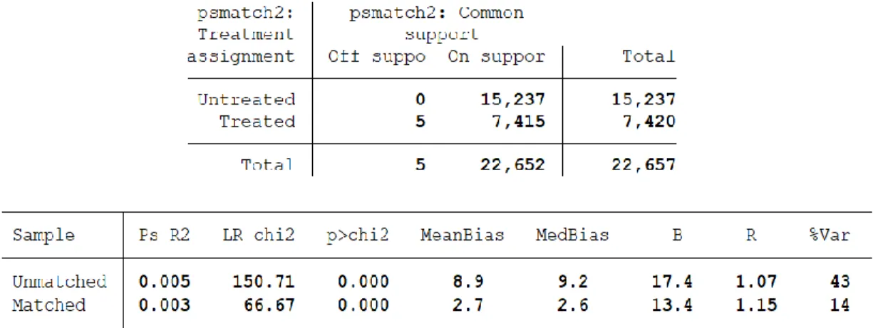
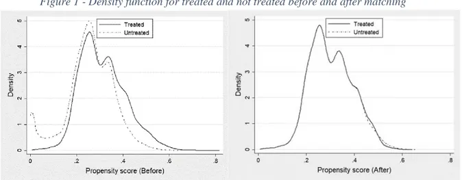
households in the Bank of Italy, has been extracted, for which both the income data and the micro-data on consumption are thus available. The households’ matching leads to an average error of 2.7 per cent, well below the 10 per cent usually accepted in literature (see Table 1 and Figure 1):
Table 1 - Propensity Score Matching results and statistics
22
Figure 1 - Density function for treated and not treated before and after matching
Source: Author’s elaboration on ISTAT and Bank of Italy data.
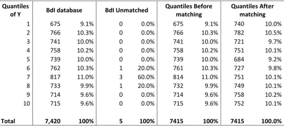
Some descriptive statistics in the following tables highlights the composition of the
database, before and after matching. After matching, the percentage of Households belonging to
each decile of income seems to be higher for the first two and the last three deciles, while it is
lower for the middle of the distribution (see Table 2). Differences are mainly attributable to the
different weights used: before matching, the deciles are constructed by the Bank of Italy (Table 2,
by column) using the weights to return each family to the universe. After matching, the information
of the selected households is traced back to the universe according to the weights of the ISTAT
database. The 5 unmatched households belong to the upper part of the income classes (Table 3).
Table 2 – Number of Households’ per income decile before and after matching
quantiles Before matching
of y 1 2 3 4 5 6 7 8 9 10 Total After matching 1 675 65 0 0 0 0 0 0 0 0 740.0 2 0 701 81 0 0 0 0 0 0 0 782.0 3 0 0 660 61 0 0 0 0 0 0 721.0 4 0 0 0 697 54 0 0 0 0 0 751.0 5 0 0 0 0 684 0 0 0 0 0 684.0 6 0 0 0 0 1 726 0 0 0 0 727.0 7 0 0 0 0 0 35 716 0 0 0 751.0 8 0 0 0 0 0 0 98 651 0 0 749.0 9 0 0 0 0 0 0 0 81 677 0 758.0 10 0 0 0 0 0 0 0 0 37 715 752.0 Total 675 766 741 758 739 761 814 732 714 715 7415.0
23
Table 3 – Percentage of Households’ per income decile before and after matching
Quantiles
of Y BdI database BdI Unmatched
Quantiles Before matching Quantiles After matching 1 675 9.1% 0 0.0% 675 9.1% 740 10.0% 2 766 10.3% 0 0.0% 766 10.3% 782 10.5% 3 741 10.0% 0 0.0% 741 10.0% 721 9.7% 4 758 10.2% 0 0.0% 758 10.2% 751 10.1% 5 739 10.0% 0 0.0% 739 10.0% 684 9.2% 6 762 10.3% 1 20.0% 761 10.3% 727 9.8% 7 817 11.0% 3 60.0% 814 11.0% 751 10.1% 8 733 9.9% 1 20.0% 732 9.9% 749 10.1% 9 714 9.6% 0 0.0% 714 9.6% 758 10.2% 10 715 9.6% 0 0.0% 715 9.6% 752 10.1% Total 7,420 100% 5 100% 7415 100% 7415 100.0%
Source: Author’s elaboration on ISTAT and Bank of Italy data.
After the matching, a matrix of information related to income, wealth and consumption for
each decile was obtained. In particular, a matrix of 485 consumption headings was therefore
obtained for ten income categories. In order to link the 485 COICOP items to the 63 NACE
activities, the correspondence matrix published by Eurostat between COICOP 1999 and CPA 2009
was used, whereby item by item the expenditure has been charged to the relevant activity. A
particular characteristic of the ISTAT questionnaire is also the possibility to retrieve information
on where goods are purchased by households, so to have the possibility to charge goods to the
relevant activities, if more than one is suitable. For some items, an imputation criterion was also
used based on information from other sources.
The methodology has therefore led to the expansion of the household consumption column
in 10 columns, resulting in the consumption per product per each decile of income.
On the value added side, the values were expanded into 10 categories, using the data on households’ wealth extracted from the SHIW which, combined with the data from the Ministry of Economy and Finance on the taxes paid, allowed also the taxes paid by consumer and producer
24
In the SAM thus constructed, the first two deciles have a disposable income level below
their consumption levels, with negative savings, while the third decile has a very low savings,
equivalent to 0.7 per cent of its disposable income. This figure rises to 41 percent for the last decile,
which saves just under half of its income. The propensity to consume is 3.5 and 2.5 for the first
two deciles, respectively. The third decile has a propensity to consume 0.99, while this propensity
lowers to 0.58 for the last decile. The average propensions for the whole distribution are 0,88 for
consumption and 0,12 for savings.
In order to have a synthetic measure of inequality in income distribution, it is possible to
compare the first and last fifth of the distribution. In the hypothetical situation of perfect equality,
every fifth of the distribution would have an income share of 20 percent of the total. In the SAM
built for this work, this ratio between the incomes of the last 2 deciles and those of the first two
deciles is 6.6 (including imputed rents).
1.2.2. A static CGE model to evaluate the economic impact
The CGE model is widely used as an instrument to evaluate the impact of policy measures
within the economic system (Scrieciu, 2007). It is built as a system of simultaneous non-linear
equations that allow assessing the effects that exogenous shocks may have on resource allocation,
efficiency and welfare. Through the changes in prices and quantities of goods, as well as income
formation and redistribution among institutional sectors, the income circular flow is completely
disentangled in all its phases, highlighting the different effects of an exogenous shock in the
25
Figure 2 – Income Circular Flow
Source: Author’s elaboration.
The construction and solution of a CGE requires several steps (Shoven and Whalley, 1984)
assuming a priori that the system is in balance and that this balance is the solution of the model.
As a result, the model allows comparing an initial equilibrium situation (benchmark equilibrium)
to a counterfactual equilibrium resulting from the application of new economic policy measures.
The Social Accounting Matrix (SAM) represents the proper accounting scheme able to represent
the initial equilibrium of the economic system. It depicts the income circular flows in all its phases
and it presents a disaggregation of Households group into income deciles, providing for each decile
a representation of income structure, its distribution and redistribution, as well as consumption.
The parameters and exogenous variables of the CGE model are calibrated on the SAM flows to
measure the direct and indirect effects of a policy aimed at replacing the actual system of
progressive taxation on personal income with a flat tax. The inclusion of household’s income
26
according to their income, track policy transmission mechanisms in the income circular flow and
highlight potential change in social equality.
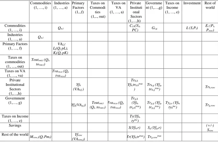
Table 4 – The structure of interactions among agents (a)
(a) Source: Author’s elaboration on Taylor (1990), Ciaschini et al. (2012).
Table 4 depicts the structure of the SAM and the interactions among economic agents.
Since the model is based on the SAM, the indices from {1 to i} indicate 63 commodities, and {1
to a} indicate 63 activities (see Appendix 1); {1 to f} denote primary factors; {1 to h} are 14
private institutional sectors (Non-financial corporations, Financial Corporations, Households
divided into deciles, Non-profit Institution serving Households, Rest of the World). Indices from
{1 to g} represent the 6 public institutional sectors (Central Government, Social Security Funds,
Regions, Provinces, Municipalities, Other Central Administrations). The SAM also include the
flows of 20 different taxes on income {1, …, e} as well as 27 taxes on output with indices {1, …,
o}. Commodities (1, …, i) Industries (1, …, a) Primary Factors (1,.,f) Taxes on Commodi ties (1,.., out) Taxes on VA (1, …, a) Private Instituti onal Sectors (1,…,h) Governme nt (1,…,g) Taxes on Income (1, …, e) Investment Rest of world Commodities (1, …, i) Qa,i Ci,h(Yh, PC) Gi,g Ii (S,Pi) Ei (Pi, Prow) Industries (1, …, a) Qa,i Primary Factors (1, …, f) Lj(QVAj pL), f,j: Kj(Qj pK) Taxes on commodities (1, …, out) Toutout,i (Qi, toout,i) Taxes on VA (1, …, va) Tvava,a (Qj, tvava,a) Private Institutional Sectors (1,…,h) Yfh (VAh,f,) Trh,h (Yfh,trh,htras ) Trh,g (Yfg, trh,gtras) Trh,row Government (1,…, g)
Yfg(VAg,f) Toutout,i
(Qi, toout,i) Tvava,a (Qj, tvava,a) Trg,h (Yfh, trg,htras) Trg,g (Yfg, trg,gtras) Tyg,e (Yfh, tyhinc) Trg,row Taxes on Income (1, …, e) Ty(Yfh, tyinc) Savings S(Yfh,r) Sg (Yfg,r) (+/-) Srow
Rest of the world
Mrow,i(Qi Pmi) Yfrow
(VArow,f) Tr(Yfh,tr
tras) Tr g,rowtras
27
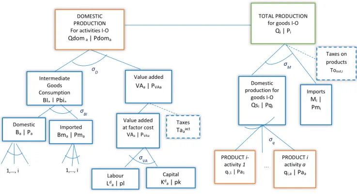
As the model formalizes the main phases of income generation, distribution and utilisation,
it is useful to start from the description of the production process (Figure 3), considering
production by activity and by product to take account of the Make-Use structure.
Figure 3. Production function by industry and by commodity.
Source: Author’s elaboration.
As for the production by activity, the functional form is a CES in different steps, in which
production inputs are combined as indicated in the left part of Figure 3. Starting from the top nest,
domestic output by activity 𝑄𝑑𝑜𝑚𝑎 is obtained combining intermediate goods 𝐵𝐼𝑎 and value
added 𝑉𝐴𝑎 as follow: 𝑄𝑑𝑜𝑚𝑎 = [𝑑𝑎𝐷𝐵𝐼𝑎𝜌𝐷 + (1 − 𝑑 𝑎 𝐷)𝑉𝐴 𝑎 𝜌𝐷] 1 𝜌𝐷 [3]
where 𝑑𝑎𝐷 is the share of intermediate goods on total production by activity, and 𝜌
𝐷 is the exponent
of the CES function linked to 𝜎𝐷. In this stage a Leontief function is assumed, thus 𝜎𝐷 ≅ 0. The
correspondent average cost function, the dual of the production function, can be written as follows:
𝑃𝑑𝑜𝑚𝑎(1 − ∑ 𝑡𝑎𝑎𝑎𝑐𝑡 𝑎𝑐𝑡 ) = [𝛿𝑎𝐷𝑃𝑏𝑖𝑎 (1−𝜎𝐷)+ (1 − 𝛿 𝑎𝐷)𝑃𝑣𝑎𝑎 (1−𝜎𝐷)] 1 (1−𝜎𝐷) [4]
Where 𝑃𝑑𝑜𝑚𝑎 is the output price for each industry, 𝑡𝑎𝑎𝑎𝑐𝑡 represents tax rates on activity, 𝛿 𝑎𝐷 is
the share of intermediate goods on total production, 𝑃𝑏𝑖𝑎 is the price of intermediate goods used PRODUCT i- activity 1 qi,1 | Pa1 Domestic production for goods I-O Qsi | Pqi Imports Mi | Pmi TOTAL PRODUCTION
for goods I-O
Qi | Pi σM Taxes on products Toout,i … PRODUCT i activity a qi,a | Paa σq Value added at factor cost VAa | PVAa Labour Ld a | pl Capital Kda | pk σD Intermediate Goods Consumption BIa | Pbia σVA DOMESTIC PRODUCTION For activities I-O
Qdom a | Pdoma Taxes Taaact Value added VAa | PVAa Domestic Ba | Pa Imported Bma | Pma σBI 1,…, i 1,…, i
28
by industry for production, and 𝑃𝑣𝑎𝑎 is the price of value added absorbed by each industry. In
each activity, the demand for intermediate goods 𝐵𝐼𝑎 and value added 𝑉𝐴𝑎 is determined as
follows: 𝐵𝐼𝑎 = 𝛿𝑎𝐷 𝑄𝑑𝑜𝑚𝑎 (𝑃𝑑𝑜𝑚𝑎 𝑃𝑏𝑖𝑎 ) 𝜎𝐷 [5] 𝑉𝐴𝑎 = (1 − 𝛿𝑎𝐷) 𝑄𝑑𝑜𝑚𝑎 ( 𝑃𝑑𝑜𝑚𝑎 𝑃𝑣𝑎𝑎 ) 𝜎𝐷 [6]
In the second nest of the production function, these two aggregates are formed, assuming
a combination with fixed coefficients, calibrated on the SAM. Considering only the duale, the
function cost for intermediate goods can be expressed as follows:
𝑃𝑏𝑖𝑎 = [∑ 𝛿𝑖,𝑎𝐵𝐼𝑃𝑖(1−𝜎𝐵𝐼)
𝑖 ]
1
(1−𝜎𝐵𝐼) [7]
Where 𝜎𝐵𝐼 is the elasticity of substitution between intermediate goods, which is equal to
zero; 𝛿𝑖,𝑎𝐵𝐼 is the cost share of intermediate goods on the total cost for intermediate goods per each
activity; 𝑃𝑖 is the good price deriving from market clearing condition on goods market.
Value added is obtained as a combination of the primary factors (labour and capital) and indirect
net taxes. Prices of primary factors are obtained in their respective markets from the combination
of supply and demand. The market of capital is competitive (Ciaschini et al. 2012).
The duale can be expressed as follows:
𝑃𝑣𝑎𝑎 (1 − ∑𝑣𝑎𝑡𝑣𝑎𝑣𝑎,𝑎) = [𝛿𝑎𝐿𝑝𝑙(1−𝜎𝑣𝑎)+ (1 − 𝛿𝑎𝐿)𝑝𝑘(1−𝜎𝑣𝑎)] 1
(1−𝜎𝑣𝑎) [8]
Where 𝜎𝑣𝑎 is the elasticity of substitution between labour and capital, set at 0.5218
according to Van Der Werf (2008); 𝛿𝑎𝐿 is the share of labour on value added; 𝑝𝑙 an 𝑝𝑘 are, the
prices for labour and capital, respectively.
Considering the right side of Figure 3, the production by goods can be derived considering
the main and secondary productions of each industry. Starting from the top nest, the total output
29
imperfect substitutability between domestic and imported goods (Armington, 1969). The dual cost
function is:
𝑃𝑖 (1 − ∑𝑜𝑢𝑡𝑡𝑜𝑜𝑢𝑡,𝑖) = [𝛿𝑖𝑂𝑃𝑞𝑖 (1−𝜎𝑀)+ (1 − 𝛿
𝑖𝑂)𝑃𝑚𝑖 (1−𝜎𝑀)] 1
(1−𝜎𝑀) [9]
Where 𝜎𝑀 is the elasticity of substitution between domestic and imported goods,
differentiated by goods; 𝛿𝑖𝑂 is the share of domestic output on total output by commodity; 𝑡𝑜𝑜𝑢𝑡,𝑖
is the tax rate on output by commodity; 𝑃𝑞𝑖 and 𝑃𝑚𝑖 are the prices of domestic goods and imported
goods. Price of imported goods depends on exogenous variables, 𝑝𝑤𝑚𝑖, which is the world price
of goods, 𝑡𝑚𝑖 represents the taxes on imports, and 𝐸𝑋𝑅, which is the exchange rate.
𝑃𝑚𝑖 = 𝑝𝑤𝑚𝑖(1 + 𝑡𝑚𝑖)/𝐸𝑋𝑅 [10]
The demand for imports depends on the total demand and on relative prices:
𝑀𝑖= (1 − 𝛿𝑖𝑂) 𝑄𝑖 ( 𝑃𝑖 𝑃𝑚𝑖)
𝜎𝑀
[11]
Moving from the production to the Income distribution part of the model, a detailed
description of the flows determining the disposable income by Institutional Sector is provided. To
consider only the main equations of the model (See Appendix 2 for a complete list of variables
and equations), starting from Households and NPISHs (their behaviour can be considered similar),
they maximise their utility function 𝑈ℎ by deciding whether they consume (𝐶ℎ) or save (𝑆ℎ): 𝑈ℎ = (𝐶ℎ𝜎𝑈−1𝜎𝑈 + 𝑆ℎ 𝜎𝑈−1 𝜎𝑈 ) 𝜎𝑈 𝜎𝑈−1 [12]
subject to the constraint of disposable income 𝑌ℎ:
𝑌ℎ = 𝑌𝐹ℎ(1 − ∑𝑖𝑛𝑐𝑡𝑦ℎ𝑖𝑛𝑐− ∑𝑡𝑟𝑎𝑠𝑡𝑟ℎ𝑡𝑟𝑎𝑠) + ∑ℎℎ∑𝑡𝑟𝑎𝑠𝑡𝑟ℎℎ𝑡𝑟𝑎𝑠𝑌𝐹ℎℎ+ ∑ 𝑇𝑟𝑔 𝑔+ 𝑇𝑟𝑟𝑜𝑤 [13]
Where Households’ and NPISHs disposable income is derived from compensation of primary
factors: 𝑌𝐹ℎ = 𝐿ℎ𝑝𝑙 + 𝐾ℎ𝑝𝑘 [14]
net of income taxes (𝑡𝑦𝑐𝑜𝑛𝑠𝑖𝑛𝑐 ) and transfers to (𝑡𝑟𝑐𝑜𝑛𝑠𝑡𝑟𝑎𝑠) and from other institutional sectors
30
The disposable income of Financial and non-financial corporations follows the same rules, with the difference in primary factors because they receive only the rent of capital:
𝑌𝐹ℎ = 𝐾ℎ𝑠𝑝𝑘 [15]
Public Institutional Sector behaviour is modelled according to the different structure of Central and Local Government in terms of different disposable income and deficit.
𝑌𝐹𝑔= 𝐾𝑔𝑠𝑝𝑘 + 𝜆
𝑔𝑎𝑐𝑡∑𝑎𝑐𝑡∑ (𝑡𝑎𝑎 𝑎𝑎𝑐𝑡⋅ 𝑃𝑎𝑎⋅ 𝑋𝑎)+ 𝜆𝑔𝑣𝑎∑𝑉𝐴∑ (𝑡𝑣𝑎𝑎 𝑎𝑉𝐴⋅ 𝑃𝑣𝑎𝑎 ⋅ 𝑉𝐴𝑎) +
𝜆𝑔𝑜𝑢𝑡∑𝑜𝑢𝑡∑ (𝑡𝑞𝑖 𝑖𝑜𝑢𝑡⋅ 𝑃𝑖⋅ 𝑄𝑖)+ ∑ ∑ℎ 𝑖𝑛𝑐𝑡𝑦ℎ𝑖𝑛𝑐𝑌𝐹ℎ [16]
where: 𝑌𝐹𝑔 is the primary income earned by each level of Government 𝑔; 𝜆𝑔𝑎𝑐𝑡 is the share of tax
revenues on activities for each level of Government; 𝜆𝑔𝑣𝑎 is the share of tax revenues on value
added for each level of Government; 𝜆𝑔𝑜𝑢𝑡 is the share of tax revenues on commodities for each
level of Government. The disposable income by Government, 𝑌𝑔 is obtained adding/subtracting the transfers from/to other Institutional Sectors (including Rest of World and other levels of Government).
𝑌𝑔 = 𝑌𝐹𝑔+ ∑ 𝑇𝑟ℎ ℎ+ 𝑇𝑟𝑟𝑜𝑤− ∑ 𝑇𝑟𝑔 𝑔 [17]
Reverting to the utility function, it can also be considered in its dual form, where the price
of utility 𝑃𝑢ℎ is given by:
𝑃𝑢ℎ = [𝛽ℎ𝑈 𝑃𝑐ℎ (1−𝜎𝑈) + (1 − 𝛽ℎ𝑈) 𝑟(1−𝜎𝑈)] (1−𝜎𝑈)1 [18] Where 𝛽ℎ𝑈 = (𝐶ℎ 𝑌ℎ) 𝜎𝑈
is the share of consumption on disposable income for each institutional
sector ℎ; 𝑃𝑐ℎ is the index price of the consumption bundle purchased by each Institutional sector
ℎ; 𝜎𝑈 is the elasticity of substitution between consumption and savings, and 𝑟 is the price of
gross savings. The demand of consumption 𝐶ℎ and savings 𝑆ℎ by institutional sector
corresponds to: 𝐶ℎ = 𝛽ℎ𝑈 𝑈ℎ (𝑃𝑢ℎ 𝑃𝑐ℎ) 𝜎𝑈 [19] 𝑆ℎ = (1 − 𝛽ℎ𝑈) 𝑈ℎ (𝑃𝑢ℎ 𝑟 ) 𝜎𝑈 [20]
31
The closure of the model consists into a set of equations related to: i) the conditions on
commodity markets, ii) the Saving-Investment balance, iii) the Rest of the World balance, iv) the
conditions on primary factors markets, v)the Government balance.
The market of each commodity is perfectly competitive, and the commodity price is
flexible to balance demand and supply:
𝑄𝑖 = ∑ 𝑏𝑖𝑎 𝑖,𝑎+ ∑ 𝑐ℎ 𝑖,ℎ+ ∑ 𝑔𝑔 𝑖,𝑔+ 𝐼𝑖+ 𝑒𝑖 [21]
Where the total supply by commodity is allocated between intermediate and final
consumption, investment and exports, following a Constant Elasticity of Transformation (CET)
function. Investment is supposed to be saving-driven:
∑ 𝐼𝑖 𝑖 = ∑ 𝑆ℎ ℎ+ ∑ 𝑆𝑔 𝑔+ 𝑆𝑟𝑜𝑤 [22]
Government and Rest of world savings are fixed, thus changes in the level of investment
depend on the savings of Households, NPISHs, financial and non-financial Corporations. The
condition for the balance of Rest of World imposes that gross saving is fixed in nominal terms.
As for primary factors, market of capital is competitive, so the rent of capital allows the
balance between demand (endogenous) and supply (exogenous). The market of labour is assumed
to be not competitive.
Full details of the model can be found in Appendix 2.
1.3. Income tax reform: implementation and results
The Italian PIT (IRPEF) was established in 1973 as a personal and progressive tax, the
precondition for which is income, in cash or in kind, falling within the categories set out by law.
Taxable persons are both resident (for income owned in Italy and abroad) and not resident in Italy
(limited to income produced in the territory of the State). The taxable amount on which the tax
32
only income produced in the territory of the State is taxable. The tax period for PIT purposes is
the calendar year.
Table 5 – Structure of the actual income tax in Italy (a)
(a) Source: Ministry of Economy and Finance.
The present work simulates the introduction of a flat rate tax applied to household’s
income. The idea follows a long-standing debate on the restructuring of the Italian personal income
tax (PIT), moving from a progressive system (as reported in Table 5) to a flat system, with a single
rate that would apply to family income, rather than on individual income.
In this perspective, three possible scenarios are assumed.
- Scenario 1 – the tax rate is 23 per cent. According to the data published by the Ministry of
Economy and Finance, the value of 23 per cent represents the middle of the distribution of average deciles’ tax rate, weighted with the number of taxpayers for each decile. Even though the new income tax revenue is below the benchmark value, we assume that the
Government operates in deficit.
- Scenario 2 – the tax rate is 23 per cent and the Government provide a provision to
compensate for the loss of revenue.
- Scenario 3 – the tax rate corresponds to the actual average income tax rate of 26.5 per cent,
which guarantees ex ante the same income tax revenue as in the benchmark.
Income in euro Tax rate Income tax
Up to 7,500 (8,000 for pensioners) - No-tax area
Until 15,000 23% 23% of the income
Between 15,001 and 28,000 27% 3,450 + 27% on the part over EUR 15,000
Between 28,001 and 55,000 38% 6,960 + 38% on the part over EUR 28,000
Between 55,001 and 75,000 41% 17,220 + 41% on the part over EUR 55,000
33
In each scenario it is possible to obtain the impact of the shift in taxation on the main
macroeconomic variables, on tax burden as well as the impact on equity, measured as the ratio
between the disposable incomes of the two extreme classes of the deciles distribution. Results are
expressed as percentage change from the benchmark represented by the SAM. The benchmark is
the counterfactual, and each scenario differs from the benchmark only for the introduction of the
flat tax, while the no-tax area and transfers from the government to households are left unchanged.
All the simulations imply that income taxation is shifted from the upper to the lower part
of the deciles’ distribution and this generates various effects on the economic system. The impact
stems from the changes in the disposable income of institutional sectors, because of different level
of income taxation compared to the benchmark. The change in the disposable income affects
consumption, savings and investments, under the assumption that all these channels operate
simultaneously.
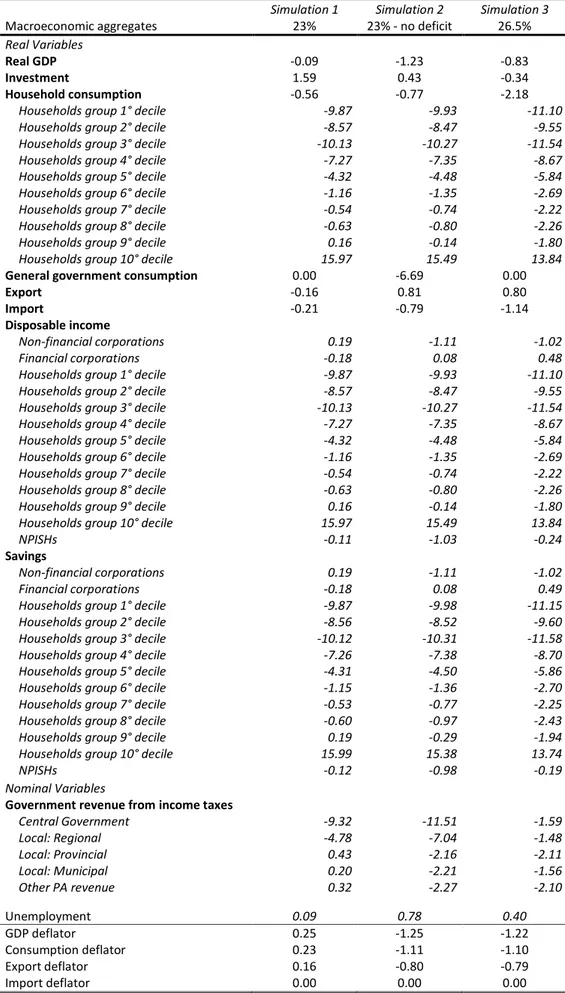
Results for Scenario 1 are shown in second column of Table 6. The introduction of a unique
tax rate of 23 per cent determines a reduction of real GDP of 0.1 per cent. This reduction derives
from the contraction of final consumption, notwithstanding the rise in real investment. The
contraction of the final consumption stems from a reduction of disposable income of the first 8 Households’ income deciles while, as expected, income of wealthier Households (9th and 10th deciles) shows an opposite result and, albeit the latter deciles have a lower propensity to consume
compared to the first ones, the increase of their income indirectly feeds the raise in investment
through an increase of savings. The increase in investments is strictly linked to how investments
and savings decisions are modelled: the closure rule of the model follow the neoclassical approach,
where investment is savings-driven, thus gross fixed investment depends on gross savings.
Moreover, a slight contraction in employment is registered (-0.1 percent), while the slowdown in
economic activity and the loose rise in deflators lead to an improvement in the current balance.