UNIVERSITÀ POLITECNICA DELLE
MARCHE
Fabrication Induced Residual Strains in Thin Composite
Laminates
Ilaria Poggetti
Supervisor: Dr. Jack Dyson
Prof.Valeria Corinaldesi
Corso di Dottorato in Ingegneria Industriale:
Curriculum in Ingegneria dei Materiali
This dissertation is submitted for the degree of
Doctor of Philosophy
Acknowledgements
Every scientific enterprise is a complex journey through the thoughts and ambitions of the individual. No journey is complete without companions and teachers.
Looking back, I would like to recognize the incomplete student who started this walk three years ago from the perspective of a much more complete individual today. Of the many experiences and teachers that make an individual a success, there are several without whom it could never have been possible.
I would like to remember with especial regard Pierpaolo Bellacima who has supported me tirelessly for these three long years. Not a morning or night has passed during this time where he has not had to suddenly awaken and come to fix this or that at a moments beckoning. Operating silently and unknown in the backwaters, often picking up the pieces with me when things wouldn’t work - I thank him sincerely for making this this possible for me.
To do a PhD, you need a home and I might add, a place to think in peace. There is a man at the Universita Politecnica delle Marche called Professor Gianni Albertini who gave me just that - a place to breathe and develop at my own pace. He encouraged me with kindness when I needed it and remained actively engaged in the background, solving the many administrative difficulties I have unfortunately encountered. Like Pierpaolo, without his kindenss and care, this would have been a bridge too far for me.
Life is full of reflections, and one such reflection is my year long stay at the University of Manchester in England where I was fortunate enough to have my first professional foreign experience. Much like Gianni, Professor Costantinos Soutis gave me a place where I could do more than just think, I could bring to life scientific thoughts using very expensive laboratories to see if they were true. Thanks also go to Dr Matthieu Gresil for advising on optical fibers and Neha Chandarana for assisting with the fabrication process and other laboratory work.
Climbing a mountain can be an easy task ... with the right equipment of course. There are two things I know about mountain climbing: not knowing an essential thing today can be fatal tomorrow. Climbing upto the the heights of a PhD degree is a similar experience and a good teacher and guide is therefore essential. Dr Jack Dyson of the Universita Politecnica delle Marche is an expert at showing me how to climb tall mountains. If I am here today, so is he, and that is all that needs to be said.
Abstract
The broad scope of this research is aimed at understanding experimentally and theoretically the factors that affect the formation of residual strains that are found to occur during the curing of carbon fiber composite plates of advanced layup geometry. We discuss results obtained during the manufacture of a standard test plate made of 5 harness satin woven carbon fiber sheets bonded with epoxy resin.
The phenomenon of residual strains that develop during the production of carbon fiber composites is one of the most significant problems in the industry. The necessity of high quality, large volume production lines for advanced applications demands that manufacturing processes be subject to norms of ever increasing precision and monitoring in an attempt to improve material performance and suitability.
The present study combines and extends the state of the art to include the effects of cure kinetics, internal force distributions and mold constraints present during the manufacturing process of polymer resin carbon fiber fabric sheets.
The chosen objective of this work is the investigation of residual strains in woven fabrics taking into account the modified kinetics of cure, the revised balance of internal forces, the viscoelastic behavior and the cure temperature profile specifically adapted to the practical case of a woven fabric composite like the 5 harness satin weave sheet.
Since many factors affect residual strain formation, the methodology of choice is a semi-analytical numerical simulation that extends the work of Hyer and Hahn, principally by modifying the matrices of the classical theory and integrating them with ideas from theoretical work already carried out on weave fabrics.
Using this approach, we show that the thermodynamics of woven composite fabrics can be characterized in closed form based on the mechanics and chemical kinetics of the manufacturing processes. Taking into consideration the morphology of the basic (weave) constituents these models permit accurate prediction of the composite properties expected from the global material structure.
The correspondence between the predicted and experimental values of strain shows an accurate physical understanding of the origins of the measured data for the entire thermal curing cycle used in the experiment.
Table of contents
List of figures xiii
List of tables xvii
1 Introduction 1
1.1 Objectives and Scopes of the dissertation . . . 1
2 State of Art 5 2.1 Composite materials . . . 5
2.2 Matrix . . . 5
2.2.1 Metal matrix composites . . . 6
2.2.2 Ceramic matrix composites . . . 7
2.2.3 Polymer matrix composite . . . 7
2.2.3.1 Epoxy Resin . . . 8 2.2.3.2 Curing Agents . . . 9 2.2.3.2.1 Amine . . . 10 2.3 Polymerization Process . . . 11 2.3.1 Cure Kinetics . . . 12 2.3.1.1 Kamal Model . . . 13 2.4 Matrix characterization . . . 13 2.4.1 TGA . . . 14 2.4.2 DTA . . . 14 2.4.3 DSC . . . 15 2.4.3.1 Heat flux DSC . . . 16 2.4.3.2 Power compensation DSC . . . 16 2.5 Reinforcement . . . 17
2.6 Textile fabrics and Woven Fabric . . . 19
2.6.1.1 Plain fabrics . . . 19
2.6.1.2 Twill fabrics . . . 20
2.6.1.3 Satin fabrics . . . 20
2.6.2 3D Woven fabrics . . . 21
2.6.2.1 Orthogonal fabrics . . . 21
2.6.2.2 Angle interlock fabrics . . . 21
2.7 Modeling of woven fabrics . . . 21
2.7.1 Mosaic Model . . . 24
2.7.2 Crimp Model . . . 28
2.7.3 Bridging model and experimental confirmation . . . 31
2.8 Composite manufacturing processes . . . 33
2.8.1 Autoclave . . . 33
2.8.2 Out-of-autoclave (OoA) methods . . . 33
2.8.2.1 Hand layup . . . 34
2.8.2.2 Pultrusion . . . 34
2.8.2.3 Liquid composite molding process . . . 35
2.8.2.3.1 Rtm . . . 35
2.8.2.3.2 Vacuum Assisted Resin Infusion Moulding . . . 36
2.9 Residual deformation after manufacturing . . . 37
2.9.1 Raw materials . . . 37
2.9.2 Cured composite part . . . 38
2.9.3 Structural health monitoring in composite . . . 39
2.9.4 Methods of Non-Destructive Techniques . . . 40
3 The experimental and model methodologies 41 3.1 Experimental Set-up . . . 41
3.1.1 Resin System characterization . . . 41
3.1.1.1 Preparation . . . 42
3.1.1.2 Experiments . . . 42
3.1.1.3 Isothermal DSC Experiments . . . 42
3.1.2 Panel manufacture experiment . . . 43
3.1.2.1 Preparation of Materials: Woven fabric reinforcement . . 45
3.1.2.2 Preparation of Materials:Mould surface preparation . . . 45
3.1.2.3 Embedded the OrFDR in the woven fabric and set-up LUNA ACQUISITION SYSTEM . . . 46
3.1.2.4 Bagging process and vacuum application . . . 48
Table of contents xi
3.1.2.6 Infusion process . . . 49
3.2 Resin characterisation model . . . 50
3.2.1 The Kamal Model application on resin system . . . 50
3.2.2 Panel manufacture experiments . . . 53
3.2.3 Static fluid expansion . . . 54
3.2.4 General theory of reacting fluids . . . 55
3.2.5 Reduction of the fluid model . . . 59
3.2.6 Adhesive clustering and polymer condensation . . . 62
3.3 Resin-Embedded optical fibre characterisation model . . . 65
3.4 Resin-Embedded optical fibre- 5HS substrate characterisation model . . . . 70
3.4.1 Ishikawa viscoelastic CLT . . . 75
3.5 Conclusions . . . 86
4 Residual strain minimization 89 4.1 Residual strain . . . 89
4.1.1 Understand and minimize the residual strain . . . 89
4.1.2 Monitoring the residual strain by viscoelastic analysis . . . 90
4.1.3 Distributed fiber strain monitoring and Strain-time relation . . . 93
4.2 Cure process . . . 97
4.2.1 Cure Cycle:cooldown phase plate 2 . . . 99
4.2.2 Cure Cycle:cooldown phase plate 3 . . . 99
4.2.3 Strain vs Temperature:Hysterisis on the thermal plane . . . 101
4.3 Curvature . . . 102
4.3.1 Inversion of curvatures . . . 104
4.3.2 Slow rate cooldown reduction of curvature . . . 105
4.4 Influence of tool/part interaction . . . 106
4.5 Conclusions . . . 106
5 Conclusions and Future Work 109 5.1 Conclusions . . . 109
5.2 Future Work . . . 112
List of figures
2.1 Classification of composites based on matrix materials . . . 6
2.2 Thermosets polymerization . . . 12
2.3 Schematic of geometrical and spatial characteristics of reinforcements in composites . . . 17
2.4 Examples of woven fabric patterns . . . 20
2.5 Examples of woven fabric patterns . . . 22
2.6 The mosaic model. . . 24
2.7 Fibre undulation model. . . 28
2.8 oncept of the bridging model. . . 32
2.9 RTM Process . . . 35
2.10 VARIM Process . . . 37
3.1 DSC dynamic scan at a heating rate of 10 °Cmin−1. . . 43
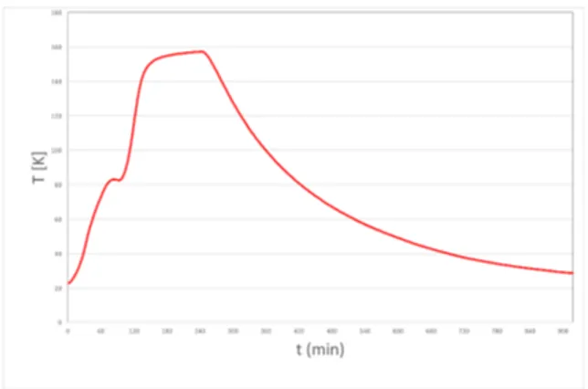
3.2 The non isothermal temperature curing cycle used in the first manufacturing experiment. . . 44
3.3 The non isothermal temperature curing cycle used in the second manufactur-ing experiment. . . 44
3.4 The non isothermal temperature curing cycle used in the third manufacturing experiment. . . 44
3.5 The green flash tape placed along the fabric’s edges. . . 45
3.6 Embedded optical sensor and composite panel geometry. . . 47
3.7 Embedded optical sensor and composite panel geometry. . . 48
3.8 The maximum degree of cure, αmaxfit and data values. . . 51
3.9 The m, n fit and data values as a function of temperature. . . 52
3.10 The rate constant logarithms ln K1, ln K2as a function of inverse temperature. 52 3.11 The LY564/HY2954 resin system thermo-kinetic surface derived from the DSC measurements. Note how the maximum cure triangle rate limits the chemical reaction. . . 53
3.12 The isothermal and non-isothermal LY564/HY2954 resin system curing parameter variation derived from the DSC measurements. . . 54 3.13 The non isothermal temperature curing cycle used in the manufacturing
experiment. . . 55 3.14 The non isothermal α curing parameter derived as a function of time from
the isothermal DSC experimental Kamal model of the LY564 epoxy resin used in manufacturing the panel. . . 55 3.15 Epoxy DGEBA/3DCM system. . . 62 3.16 DGEBA synthesis reaction. . . 63 3.17 The optical fiber inside the resin system, I resin system suspension, II resin
system suspension and adhesion, III resin system adhesion. . . 66 3.18 The mathematical representation of the CTE of control volume Γ. The rapid
rise of this curve indicates that very little time is needed before there is enough cured resin enveloped around the optical fibre to curtail its intrinsic mechanical contribution. . . 68 3.19 The embedded mean optical fibre infusion strain at t = 0 (top line, black)
undergoes a near constant downward shift in each section by the end of the manufacturing process. The original strain signal including noise is in gray. 69 3.20 The optical fiber inside the resin system. Inset shows the Γ control volume
CTE as a function of surface condensation in a unit cell of 5HS homogenised laminate. It is the equivalent of figure 3.17 for a plate substrate geometry. . 69 3.21 A comparison of standard Ishikawa CLT equation 3.99 with the modified
Ishikawa CLT of equation 3.100 with embedded optical fibre strain signal during panel manufacture. . . 74 3.22 The CTE of the resin structure derived from figure 3.21 as a function of
temperature. This the equivalent of figure 3.21 for a 5HS unit cell surface control volume Γ. See figure 3.18. . . 74 3.23 Undulation unit cell for an Ishikawa one dimensional weave model with
idealised h1h2shape functions. . . 78
3.24 The real h1(x) and h2(x) shape functions used in calculating the Ishikawa
unit cell for the 5HS weave used in the experiment. . . 78 3.25 Unit cell for an Ishikawa one dimensional bridge structure. . . 82 3.26 Tri-curve determination of the glass transition temperature. . . 85 3.27 Comparison of the complete panel manufacture strain-temperature optical
fibre data and equation 3.99. . . 85 4.1 Schematic of life cycle monitoring approach for a laminate[20] . . . 94
List of figures xv
4.2 Microstrain compare between the second and third plate. . . 95
4.3 Second plate microstrain in the top(green), middle(red) and bottom(blue) layers. . . 95
4.4 Third plate microstrain in the top(green), middle(red) and bottom(blue) layers. 96 4.5 Distributed strain plate 3 . . . 96
4.6 Cure cycle plate 2. . . 98
4.7 Cure cycle plate 3. . . 98
4.8 Cooldown phase for the second plate laminate . . . 100
4.9 Cooldown phase for the third plate laminate . . . 100
4.10 The cooldown phase compare between the second and third plate laminate . 101 4.11 Second and third plate microstrain variation with Temperature. . . 103
4.12 Second plate microstrain variation with Temperature in the top(green), mid-dle(red) and bottom(blue) layers. . . 103
4.13 Third plate microstrain variation with Temperature in the top(green), mid-dle(red) and bottom(blue) layers. . . 104
4.14 Mean values strain (top, middle and bottom layers) in Second and Third plate 105 4.15 Mean values strain (top, middle and bottom layers) in Second and Third plate compare with an ideal new plate . . . 107
4.16 The cooldown phase compare between the second and third plate and an ideal New plate laminate . . . 108
4.17 The cooldown phase compare between the second and third plate and an ideal New plate laminate . . . 108
5.1 Mean values strain (top, middle and bottom layers) in Second and Third plate compare with an ideal new plate . . . 113
5.2 The cooldown phase compare between the second and third plate and an ideal New plate laminate . . . 114
5.3 The cooldown phase compare between the second and third plate and an ideal New plate laminate . . . 114
List of tables
Chapter 1
Introduction
1.1
Objectives and Scopes of the dissertation
Polymer composite products are increasingly applied in demanding structures in the aerospace and the aeronautical industry.
The quality and the performance of a composite part are determined by the manufacturing cycle that is accompanied mainly by the exothermal polymerization reaction of the thermoset resin. Due to the continuous variation of the resin mechanical and rheological properties, it is extremely important to ensure a uniform evolution of the cure reaction that, coupled with the heat transport conditions, can lead to exothermal peaks, thermal and chemical conversion gradients determining residual strain and gradients of the matrix mechanical properties.
Residual strain can distort the dimensions or shape of the processed part, necessitating expensive compensation through the use of shims when it is assembled into a structure. The advancement of the cure reaction implies the consolidation of the polymer resin which changes its physical state passing from a low molecular weight liquid to a rubbery solid and, then at length transforming into a glassy at the end of the processing cycle through chemical reactions of the active groups present in the system which develop progressively a denser polymeric network until reaching the so-called gel point and forming an insoluble material. Therefore, due to the continuous variation of the resin mechanical and rheological properties, it is extremely important to ensure a uniform evolution of the cure reaction that, coupled with the heat transport conditions, can lead to exothermic peaks, thermal and chemical conversion gradients determining residual strain and gradients of the matrix mechanical properties. Residual stresses and strains can distort the dimensions or shape of the processed part, necessitating expensive compensation through the use of shims when it is assembled into a structure. Liquid Composite Molding (LCM) processes are therefore the focus of this thesis, where liquid resin is injected through a textile preform. Using a distributed embedded
optical fiber sensor it has been possible to extract real time monitoring of the curing process and as a direct result the gellification of a thermo-set matrix. The aim of this work is to understand how residual strains build up during such processing. Furthermore, different modeling approaches, constitutive models and experimental techniques are investigated with the objective of understanding the various mechanisms taking place during the process and what light simple mathematical models can shed on them. A number of studies have been conducted to optimize the process cycle to objectively minimize the linear strains inside the composite materials, but it will shown that the formation of stresses and strains during manufacturing are dependent upon the quasi-liquid like composition of the composite structure before gellification and beyond that, upon solidification of the resin, the type of cooling profile that is applied.
Experimental results show in particular that the commonly held view that a variational analysis of the cooling problem for composite manufacturing can provide an optimal path over which strains are minimal during and after the cooling phase is unrealistic. Mathematically this is no surprise, since the solution to the integro-differential equations involved is possible under certain circumstances and these seem to be unphysical at best.
The experiments conducted over two different cooling schemes, one slow and the other fast, do however show that the sign of the curvature in the final cooled down plate is inverted. If the cooling problem is mathematically stable in the sense that it is a continuous function of the cool down temperature process, then the experimental results we have could be significant. That is because these results show that there must be a real cool-down curve as yet not specified that permits the manufacture of a plate with zero plate curvature but nonetheless a constant strain present in the composite plate at the end of manufacture. This immediately implies the existence of a suitable theoretical framework that can practically lead to optimal cooling solutions for plate curvature problems. That, be that as it may, is a future objective for both ourselves and perhaps other researchers in the field.
For about thirty years the precise effect of the liquid state resin upon optical fiber or other methods of measurement has been subject to speculation for example, and in this study we attempt to provide a simple model and experimental evidence to come the conclusion that in fabrication processes for composite materials it is highly likely that the optical fiber always measure the true strain.
The present study contributes to a better understanding of the physics of resin rheology by proposing a simple physical theory that could lead to improved composites design. A better model of resin rheology leads one directly to a precise understanding of the gellation process during the second dwell of the curing cycle and the glass transition temperature.
1.1 Objectives and Scopes of the dissertation 3 Subsequently this may have a significant impact upon the way the cooling cycle operates on the stresses in the relaxed structure.
Furthermore, and perhaps more significantly, we observe and explain that the presence of carbon fiber structures within a resin matrix strongly modify the rheology and hence the residual strain behavior In particular we precisely identify how this new rheology operates in terms of a physical mechanical mechanism. The originality of the substrate strain model proposed lies in the fluid-chemical action of the curing resin when it is considered as a distributed adhesive. This simple fact leads directly to a thermodynamic non extensive modification of the strain response of the composite material which is encapsulated in the pseudo-liquid state equation for connecting the solid state and liquid-state composite coefficients of thermal expansion1.
Chapter 2
State of Art
2.1
Composite materials
A composite is a combination of two or more component materials, with different properties and different forms through compounding processes, it not only maintains the main charac-teristics of the original component, but also shows new character which are not possessed by any of the original components [78]. Composite materials should have the following characteristics:microscopically it is non-homogeneous material and has a distinct interface; there are big differences in the performance of component materials and the formed com-posite materials should have a great improvement in performance. Comcom-posite material is a multi-phase system consisted of matrix material and reinforcing material. Reinforcing material is a dispersed phase, usually fibrous materials [78]. The fibres most frequently used are Glass, Aramid and Carbon and in some very special applications Boron fibres. These are usually in the form of long continuos filaments knows as “UD” or unidirectional tape where the fibres run in one direction only or woven into fabric, wich can be various styles of weave, weight and fibres orientation.
2.2
Matrix
The matrix is the material used to bind all the fibres together, when the resin is cured it will form a solid, and by doing this it will hold the component rigid and distribute the load by transferring it between the fibres.Based on the matrix material, the composites are classified into polymer matrix composites (PMCs), metal matrix composites (MMCs), and ceramic matrix composites (CMCs). The three types of composites differ in the manufacturing method adopted, mechanical behaviors, and functional characteristics. Since the matrix materials
undergo physical or chemical change, the processing method to be used for making the composites has a direct bearing on the matrix system used. The polymeric matrix composite are the most common. The classification of composites based on matrix material is shown in Figure 2.1.
Fig. 2.1 Classification of composites based on matrix materials[6]
2.2.1
Metal matrix composites
Metal matrix composites (MMCs), as the name implies, have a metal matrix. Examples of matrices in such composites include aluminum, magnesium, and titanium. Typical fibers include carbon and silicon carbide. Metals are mainly reinforced to increase or decrease their properties to suit the needs of design. For example, the elastic stiffness and strength of metals can be increased, and large coefficients of thermal expansion and thermal and electric conductivities of metals can be reduced, by the addition of fibers such as silicon carbide.[52] Metals or metallic alloys are used as the matrix material in MMCs. Mainly lightweight metals and alloys such as, aluminum, titanium, and their alloys are used. In some special applications, heavy metals such as copper and cobalt are used. MMCs can be suitable for applications where the service tem perature is up to 1200°C. At present, short fibers or particulates are mainly used as the dispersed phase because of the processing advantage. Metals and alloys are also reinforced with continuous fibers to improve modulus and strength significantly. A major problem for the MMCs is corrosion. Most of the MMCs are still under development and only a few components are made commercially. Recent interest on MMCs has concentrated on transport applications and consequently the light metal-based MMCs, particularly aluminum and its alloy-based MMCs, have received the most attentio.[6]
2.2 Matrix 7
2.2.2
Ceramic matrix composites
Many oxide and nonoxide ceramic materials are used as matrix materials in CMCs. CMCs are useful for high-temperature applications, where the service temperatures are above 1200°C. These materials are very expensive because most of the CMCs are processed at high temperature. In some cases, there is a need to apply high pressure at that high temperature to get a quality product.[6]
2.2.3
Polymer matrix composite
The matrix material can be a thermoset polymer, a thermoplastic polymer, or an elastomer in the PMCs. Thermoset polymers are very commonly used because of the processing advan-tage. Currently thermoplastic polymers are gaining importance because of their relatively high toughness values and the possibility of post-processing. To meet the specific property requirements, a wide variety of thermoplastic polymers are available. PMCs are suitable for making products, which are used at ambient temperature. There are some special polymers, which can be used up to 250°C. In any case, PMCs are not suitable for applications where the service temperature is more than 350°C. The success of PMCs, largely as replacement for metals, results from the much improved mechanical properties of the composites compared to the plastic matrix materials. The good mechanical properties of the composites are a consequence of utilizing the high-strength and high-modulus fiber reinforcement.[6] Ther-moplastic flow when tey are hetated beyond a particular temperature while themoset remain in the solid state until their temperature becomes so high that degradation of the materilas takes place. The different behavior of thermosets and thermoplastics when heated arises from their chemical structures. Thermoplastic are linear polymers that in the solid state are either semicrystalline or amorphous glasses.When they are hetaed beyond the melting point of crystals or beyond the glass transition temperature polymers chains are free to move and flow takes place. On the other hand, thermosets are crosslinked polymers and they remain in the solid state as long as the covalent chemical bonds are not destroyed.[32] Due to the three dimensional network, the mechanical properties of thermosets are generally superior to those of thermoplastic materials. Moreover, thermosets possess good insulating and adhesive properties, are resistant to most chemicals and have high thermal stability. Therefore, they are commonly used as adhesive, coating or matrix for structural composites for airplanes, boats and electronic devices. Thermoplastic polymers can be melted and reformed, they have much higher strains to failure because they can undergo extensive plastic deformation resulting in singnificantly improved impact resistance.
2.2.3.1 Epoxy Resin
One of the most popular resins in use today are the epoxy resins, having the advantage of good structural strength together with the ability to withstand relatively high temperatures. Epoxy resins belong to the class of thermosetting plastics, a thermoset material cannot be melted and reformed after curing. The curing process transforms the epoxy resin into a plastic by forming a three dimensional network of covalent bonds. Curing is initiated through heat and/or curing agents hardener. The liquid resin are converted into hard brittle solid by chemical cross-linking which leads to the formation of a tightly bound three-dimensional network of polymer chains. The mechanical properties depend on the molecular units making up the network and on the length and density of cross-link. Curing can be achieved at room temperature but it is usual to use a cure schedule which involves heating at one or more temperatures for predetermined times to achieve optimum cross-linking and hence optimum properties. [39]. An epoxy is a polymer that contains an epoxide group, one oxygen atom and two carbon atoms in its chemical structure.The diglycidyl ether of bisphenol-A (DGEBA) is the most commonly used epoxy resin as it has many attractive properties such as fluidity, low shrinkage during cure and ease of processing. The cured products have good physical strength, excellent moisture, solvent and chemical resistance [44] Diglycidyl ether of bisphenol A (DGEBA) contain two epoxide groups. Hardeners are added to the epoxy prepolymers to increase the rate of polymerisation by reacting with the epoxy groups. Curing agents are organic amino or acid compounds and cross-linking is obtained by introducing chemicals that react with the epoxy and hydroxy groups between adjacent chains. The exent of cross-linking is a function of the amount of curing agent added, the curing agent become part of the epoxy structure. [12] Unreacted resins are usually referred to as A-stage resin. A partially reacted resin, usually a vitrified system below gel point is called a B- stage resin, while completely cured resin is called a C-stage resin. The essential condition to advance a thermoset resin to B-stage is vitrification prior to gelation and is achieved by keeping the reaction temperature below the curing temperature, Tc. Ease in processability is achieved by
using B-stage resin. [77] An epoxy before it is fully cross-linked is said to be in stage B and in B stage an epoxy has characteristic tackiness. This B-stage resin is used to make a fiber prepreg. The type and extent of curing agent adding will control the total curing time (also called the shelf life or pot life).[12] The resins are for the most part a combination of various chemical elements. When these elements are mixed together they start a reaction that binds the molecules together and causes the resin to become solid. The speed of this reaction is dependent on two principle factors, the first of which is the mix ratio of chemical elements; the more accelerator or catalyst that is added the faster the cure will take place. It is the ratio of these elements that set the underlying “Out Life” and “Shelf life” for the prepregs. By
2.2 Matrix 9 varing this ratio the shelf life of prepregs can be modified from six month to a year and an out of life from just a few days to six months. The second factor that controls the cure rate is the temperature. The composite industries is one of the few industries where the component is produced right at the end of the manufacturing process. In most other industries they have the raw materials at the start of manufacturing cycle and then carry out the various machining and finishing operation in order to produce the required component. The advantages that they have in this situation is that they can test the raw materials before starting the manufacturing process. If the component is not up to specification it can be rejected before any more time and effort is expended on it. But composites do not afford this luxury. When we lay our woven fabrics in the mould it is just a mass of resin and fibres that exist in the same space. Not until they are cured do we benefit from the attributes of the fibres and the resin working together with one another. In light of the above, is it clear that the manufacturing and the cure cycle process for a composite component are very delicate phases. In order to ensure that the composite material component is up to specification it is fundamental have a wide understanding of resin system and the reinforced material as well as their interaction during the manufacturing and curing process for limit and minimize the waste of components and consequently the waste of money. If the cure of the component takes place at a temperature too low the resin will not attain its full mechanical properties and the surface finish. If on the other hand the cure of the component takes place at a temperature too high the resin matrix could be degrade and it will adversely affect the strength of the component. The selection of cure cycle is essential for achieved a good quality component in term of mechanical properties and surface finish. Sometimes the composite component appears apparently very good externally but inside have a residual stresses that can affect the mechanical properties during the component life. The aim of this work will be to analyzing and understand the residual strain behavior during a complete “standard” cure and cooling cycle process and the indentification of a “special” cure and cooling cycle process that minimize the residual strain of the final composite components.
2.2.3.2 Curing Agents
In order to convert epoxy resins to hard, infusible thermoset networks it is necessary to use crosslinking agents. These crosslinkers, hardeners or curing agents as they are widely known, promote cross-linking or curing of epoxy resins. Curing can occur by either ho-mopolymerisation initiated by a catalytic curing agent or a polyaddition/copolymerisation reaction with a multifunctional curing agent.[19] The mechanical properties of the epoxy are dependent on the type of curing agent used. Acid anhydrides and multifunctional amines are most commonly used. [40] The choice of curing agent depends on processing method,
curing conditions, i.e., curing temperature and time, physical and chemical properties desired, toxicological and environmental limitations, and cost. The epoxy group, because of its three-membered ring structure, is highly reactive and can be opened up by a variety of nucleophilic and electrophilic reagents. Curing agents are either correactive or catalytic. A catalytic curing agent functions as an initiator for epoxy resin homopolymerization, whereas the co-reactive curing agent acts as comonomer in the polymerization process. A variety of curing agents containing active hydrogen atom such as aliphatic and aromatic amines, polyamide amines, polyamides, anhydrides, dicyandiamide, isocyanate, polysulphides, mercaptans, melamine-formaldehyde, urea formaldehyde, etc. have been used. [77]
2.2.3.2.1 Amine Of the many types of curing agents, amines are most widely utilized as curing agents in epoxy matrices for high performance composites. Amine compounds are classified into primary, secondary, and tertiary amines, in which one, two, and three hydrogen molecules of ammonia (NH3) have been substituted for hydrocarbon, respectively. Amines are called monoamine, diamine, tri-amine, or polyamine according to the number of amines in one molecule. Three principal reactions take place between the amine curing agent and epoxy, the reaction is between epoxy groups and primary amine leading to the production of a secondary aminde and hydroxly group, (2) the reaction between epoxy groups and secondary amine hydrogens leading to the production of tertiary amine, (3) the etherification reactions between epoxy groups and the hydroxy group. The initial reaction of a primary amine can produce a secondary one, and the subsequent reaction leads to a tertiary amine. [47] Amines are classified into aliphatic, alicyclic, and aromatic amines according to the types of hydrocarbons involved, and the all are important curing agents for epoxy resin. Aliphatic amines yield fast cure times, whereas aromatic amines are less reactive but result in higher glass transition temperatures. [40]. Aliphatic amine rapidly reacts with epoxy resin, is a representative room-temperature curing agent.Resins that have been cured using aliphatic amines are strong, and are excellent in bonding properties. They have resistance to alkalis and some inorganic acids, and have good resistance to water and solvents, but they are not so good to many organic solvents. Aromatic amine has weaker basicity than aliphatic amine and slowly cures at room temperature due to steric hindrance by the aromatic ring. The curing virtually stops in the B-stage of a linear polymer solid due to the large difference in the reaction of primary and secondary amines. Normally, the curing of aromatic amine requires heating in two steps. The first heating is carried out at a rather low temperature of approximately 80°C so as to lessen heat generation, and the second heating is carried out at a high temperature of 150°C to 170°C. Aromatic amines are often used as curing agents in epoxy prepreg resins as well as infusion resins, including those for
2.3 Polymerization Process 11 resin transfer molding (RTM), vacuum assisted resin transfer molding (VARTM), resin film infusion (RFI), pultrusion, and filament winding. Cycloaliphatic amines are also used in VARTM type composite processes and specialty RTM and filament winding. Most commonly, cycloaliphatic and aliphatic amines are used as curing agents in epoxy wet-laminating resins. Shown below is a summary of some of the main advantages and disadvantages of the different classes of amine curing agents when used in epoxy systems.
2.3
Polymerization Process
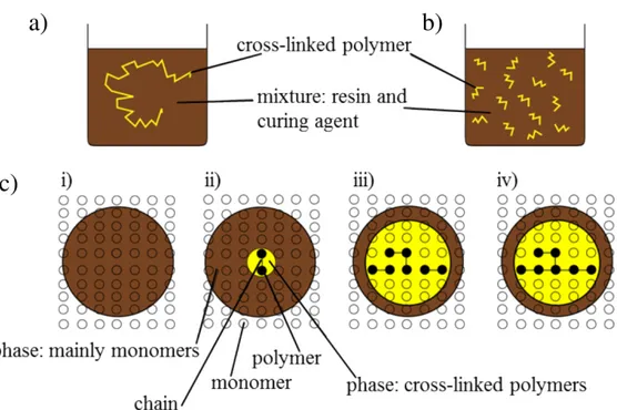
Epoxy resin system are included in the group of thermosetting polymers. Starting with the ini-tial uncured state the matrix, a mixture if resin and curing agent, undergoes a polymerization process during curing. As introduce by Flory [21] two polimerization reaction mechanism are distinguidhed: fre-radicals or ions (chain-growth polymerization) and by functional groups (step-growth polymerization) [58] . The curing of epoxy resins is associated with a change in state from a low molecular weight liquid mixture to a highly cross-linked network. The molecular mobility in the system decreases as the cure proceeds due to cross-linking of several chains into network of infinite molecular weight. [77] The molecular mobility in the system decreases as the cure proceeds due to cross-linking of several chains into network of infinite molecular weight. Figure 2.2 shows the chain-growth polymerization. In Figure 2.2 a) is shown the polymerization reaction with an initiator the unsaturated monomer molecules add onto the active site of a growing polymer chain one at time. The characteristics of step-growth polymerization are the step-growth throughout the matrix, whereas no initiator is necessary and the reaction between any two functional groups of monomers is stepwise. Thus, at multi-ple locations and at the same time similar steps are repeated throughout the reaction process as illustrated in Figure 2.2 b). In particular initiation, propagation, and termination reactions are essentially identical in rate and mechanism as shown in Figure 2.2 c). The chain length increases steadily and random growth takes place as the monomer reacts with both monomer or polymer species with equal ease until a high molecular weight polymer is obtained.[58] The transformation of low molecular weight liquid into high molecular weight amorphous solid polymer by chemical reaction is the fundamental process used in the coatings, adhesives and thermo-set industries. As the chemical reaction proceeds, the molecular weight and glass transition temperature (Tg) increase, and if the reaction is carried out isothermally below the glass transition temperature of the fully reacted system (TgINFINITO), the polymer Tg will eventually reach the reaction temperature (Tcure). During isothermal reaction below TgINFINITO, two phenomena of critical importance in thermosetting processing can occur: gelation and vitrification.[4] Gelation corresponds to the incipient formation of an infinite
Fig. 2.2 Polymerization in thermosets: a) schematic illustration b) step-growth polymerization c) step-growth polymerization adapted to i) uncured state, ii) two monomers react, iii) state with larger chain length including dimer and trimer, iv) state where branching started.
[58]
molecular network, which gives rise to long range elastic behavior in the macroscopic fluid. It occurs at a definite conversion for a given system according to Flory’s theory of gelation. After gelation the material consist of normally miscible sol(solvent-soluble) and gel(solvent-insoluble) fractions, the ratio of former to the latter decreasing with conversion. Vitrification occurs when the glass transition temperature,Tg, rise to the isothermal temperature of cure. The material is liquid or rubber when Tcure>Tg; it is a glassy when Tcure<Tg. [25]
2.3.1
Cure Kinetics
Studies on the curing kinetic characterization of the thermo-set resins are important to under-stand the relationships between the structure of the cured resin and processing techniques, as well as the properties for high performance composites.[57] In order to investigate the cure development numerically, cure kinetics models specific to the resin system used in the composite were developed. The extent of the cure reactions is usually described by the degree of cure, α, which is quantified as the fraction of heat generated to that point relative to the total heat generated through the complete cure. The degree of cure can easily be determined using standard heat flow measurements in a Differential Scanning Calorimeter
2.4 Matrix characterization 13 (DSC) by integrating the exothermic DSC peak. [88] The mechanisms of the curing reaction of thermosetting resins follow the general kinetic models,namely, n-th order and autocatalytic mechanisms.[57] The reaction rate of nth-order kinetics can be expressed as:
dα
dt = K(T )(1 − α)
n (2.1)
The reaction rate of autocatalytic kinetics can be defined as: dα
dt = K
′
αm(1 − α)n (2.2) where α is the extent of reaction, and α is given by α = ∆Ht
∆H0, where ∆Htis the partial area
under a DSC trace up to time t; m and n are the reaction orders; and K′is the kinetic rate constant.
2.3.1.1 Kamal Model
According to the n-th order kinetic model, the maximum reaction rate will be observed at time t=0; according to the autocatalytic model, the reaction rate is zero or very small initially and reaches a maximum value at an intermediate conversion. The autocatalytic kinetics was expressed by Kamal, the generalized expression is:
dα
dt = (K1+ K2α
m)(1 − α)n (2.3)
where α is the cure conversion, K1and K2are the specific rate constants that are functions of
temperature with two different activation energies and preexponential factors, and m and n are the reaction orders. [57] According to nth-order kinetic model, the maximum reaction rate will be observed at t = 0, whereas the maximum reaction rate of the autocatalytic reaction will appear at some intermediate conversion.
2.4
Matrix characterization
The exponential growth of polymer applications has led to the developmnet of several new techniques for polymer characterization, no single technique has proved more useful than thermal analysis.[76]. The standard thermal analytical techniques such as thermogravimetry (TGA), differential thermalanalysis (DTA) and differential scanning calorimetry (DSC), have been extensively used to study phase changes of materials [10]. The ability of a substance to undergo phase transitions and also the temperature intervals and heats of these transitions
can be determined from thermographic heating and cooling curves, the shape of which is different for crystalline and amorphous polymers.[27]
2.4.1
TGA
Thermogravimetry or thermogravimetric analysis is one of the most popular thermal methods. The terms are used interchangeably and often abbreviated to TG or TGA. The origins of thermogravimetric date back to 1912 when Urbain described the first equipment that could continuously heat and weigh a sample under a controlled gas atmosphere.Three years later, Honda coined the term "thermobalance" for his instrument which was also capable of reducing the heating rate when a mass change was occurring leading to a form of sample-controlled thermal analysis.Applications to polymers and pharmaceuticals blossomed after the 2nd World War and became more widespread with the introduction of commercial instrumentation beginning in th 1960s. [23]. TGA measures the amount and rate (velocity) of change in the mass of a sample as a function of temperature or time in a controlled atmosphere.The measurements are used primarily to determine the thermal and/or oxidative stabilities of materials as well as their compositional properties. The technique can analyze materials that exhibit either mass loss or gain due to decomposition, oxidation or loss of volatiles (such as moisture). It is especially useful for the study of polymeric materials, including thermoplastics, thermosets, elastomers, composites, films, fibers, coatings and paints. TGA data provide characteristic curves for a given polymer because each polymer will show a unique pattern of reactions at specific temperatures. In TGA, a sample is placed in a furnace while being suspend from one arm of a sensitive balance. The change in sample mass is recorder while the sample is maintained either at a required temperature or while being subject to a programmed heating sequence. The thermobalance can detect to 0.1 µg and calibration can be made by using standard masses.The TGA curve can be plotted as the sample mass loss as a function of temperature, or alternatively, in a differential form where the change in sample mass with time is plotted as function of temperature.
2.4.2
DTA
Differential thermal analysis (DTA) techniques permit study of thermal behavior of mate-rials as they undergo transformations as a function of temperature. The principle of the technique is that a sample and a reference material are heated while both are monitored by thermocouples. The two thermocouples produce identical voltages when there are no thermal transformations whereas when a thermal transformation occurs there is a change in this voltage. If the change is positive there is an exothermic reaction whereas a negative
2.4 Matrix characterization 15 change shows an endothermic reaction. DTA thermograms plots of this voltage change as a function of the reference temperature, provide data regarding glass transition, crystalliza-tion and melting parameters. Differential scanning calorimetry (DSC) is another thermal technique similar to DTA in the type of the information available although the experiment is more reproducible due to the nature of the instrument[71]. Differential scanning calorimetry (DSC) and Differential thermal analysis (DTA) are related techniques that measure the same thermal events with different methods. DSC monitors the difference in heat flow between a sample and reference as the material is heated or cooled while DTA measures a difference in temperature. [72] DTA involves heating or cooling a test sample and an inert reference under identical conditions, while recording any temperature difference between the sample and reference. This differential temperature is then plotted against time, or against temperature. Changes in the sample which lead to the absorption or evolution of heat can be detected relative to the inert reference. Differential temperatures can also arise between two inert samples when their response to the applied heat–treatment is not identical. DTA can therefore be used to study thermal properties and phase changes which do not lead to a change in enthalpy. The baseline of the DTA curve should then exhibit discontinuities at the transition temperatures and the slope of the curve at any point will depend on the microstructural constitution at that temperature. A DTA curve can be used as a finger print for identification purposes, for example, in the study of clays where the structural similarity of different forms renders diffraction experiments difficult to interpret. The area under a DTA peak can be to the enthalpy change and is not affected by the heat capacity of the sample. DTA may be defined formally as a technique for recording the difference in temperature between a substance and a reference material against either time or temperature as the two specimens are subjected to identical temperature regimes in an enviroment heated or cooled at a controlled rate.
2.4.3
DSC
A DSC analyser measures the energy changes that occur as a sample is heated, cooled or held isothermally, together with the temperature at which these changes occur. The energy changes enable the user to find and measure the transitions that occur in the sample quantitatively, and to note the temperature where they occur, and so to characterize a material for melting processes, measurement of glass transitions and a range of more complex events. One of the big advantages of DSC is that samples are very easily encapsulated, usually with little or no preparation, ready to be placed in the DSC, so that measurements can be quickly and easily made.The main property that is measured by DSC is heat flow, the flow of energy into or out of the sample as a function of temperature or time. [22] There are two types of DSC instruments in commercial use today. One is known as a "heat flux"design while the other
is referred to as a "power compensation"instrument.While each type has its adherents, the essential information extracted by this technique is not influenced significantly by the two approaches. In essence, both heat flux and power compensated DSC’s use a temperature difference between a sample and a reference as the raw data.Both types of DSC instruments convert temperature difference into a measurement of the energy per unit mass associated with the phase change that caused the temperature difference to arise. Any transition in a material that involves a change in the heat content of the material can be detected and measure by DSC.
2.4.3.1 Heat flux DSC
Heat flux DSC is of a single furnace design with a temperature sensor (or multiple sensors) for each of the sample and reference pans located within the same furnace; see FIGURE. Sample and reference pans are placed in their required positions and the furnace heated at the pre-programmed heating (or cooling) rate. When transitions in the sample are encountered a temperature difference is created between sample and reference. On continued heating be-yond the transition this difference in temperature decreases as the system reaches equilibrium in accordance with the time constant of the system. It is the difference in temperature or ∆t signal that is the basic parameter measured. Modern analysers are carefully calibrated so that the ∆t signal is converted to a heat flow equivalent and this is displayed as a function of temperature or time. The reason a difference in temperature is created is easily understood if melting is considered. When melting of a single crystal occurs the resulting mixture of solid and liquid remains at the melting point until melting is complete, so the temperature of the sample will fall behind that of the reference. Typical heat flux DSC analysers can be used from liquid nitrogen temperatures to a maximum of around 700 °C similar to power com-pensation DSC, though modern high-temperature DTA analysers normally offer a calibrated DTA (heat flow) signal giving a measurement derived from the heat flux to significantly higher temperatures. [22]
2.4.3.2 Power compensation DSC
Power compensation DSC has at its heart two small identical furnaces, one for the sample and one for the reference (normally an empty pan), the reference being the right-hand furnace. These are both heated at a pre-programmed heating (or cooling) rate and power compensations are applied to either furnace as required to maintain this rate. In the resulting DSC trace the difference in energy flowing into the sample furnace is compared to the inert reference and plotted as a function of temperature or time. This design measures flow of
2.5 Reinforcement 17 energy directly in mW or J s−1.Therefore the raw heat flow signal can be viewed as a form of heat capacity. In practice, it reflects the changes occurring in heat capacity, and the absolute value is obtained when the method used takes into account the contribution of the empty pans and reference together with the scan rate. The small furnaces of this system can be heated or cooled at very low rates to very high rates and are ideal for a range of different techniques, particularly fast scan DSC. Power- compensated DSC also permits true isothermal operation, since under constant temperature conditions both the sample and furnace are held isothermally. The temperature range of use is from liquid nitrogen temperatures to around 730 °C. [22]
2.5
Reinforcement
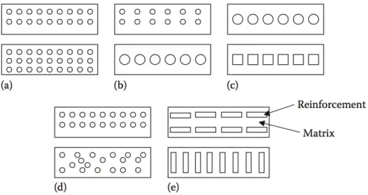
In the most general case a composite material consists of one or more discontinuous phases distributed in one continuous phase, the continuous phase is called the matrix, the discon-tinuous phase is called the reinforcement, or reinforcing material. The geometry of the reinforcement will be characterized by its shape, its size, the concentration of the reinforce-ment, its disposition (its orientation), etc. [7] These charatcteristic are illustrated in Figure 2.3 The shape of the reinforcement will be schematically approximated by either spheres or
Fig. 2.3 Schematic of geometrical and spatial characteristics of reinforcements in composites: (a concentration, (b size, (c shape, (d distribution, and (e orientation.
[6]
cylinders.The concentration of the reinforcement is usually measured by the volume fraction or by the weight fraction. The concentration of the reinforcement is a determining parameter
of the properties of the composite material. The weigth fraction is relevant to fabrication and the volume fraction is commonly used in property calculations. Weight and volume fraction are related to each other through density ρ. The size of the dispersed phase also influences the properties of composites. In general, the smaller the size, the better will be the mechanical properties, because of size effect; that is, the size of defect is restricted and it should be smaller than the size of the material. The strength of any material is inversely proportional to the size of defect. The surface area of a material depends on the size and shape. For any particular volume, the smaller reinforcement has more surface area. The contact area between reinforcement and matrix increases with surface area, resulting in better properties. [6] For a given concentration the distribution of the reinforcement in the volume of the composite is also an important parameter. A uniform distribution will ensure a "homogeneity" of the material, i.e., the properties of the composite will be independent of the point of measurement. In the case of a nonuniform distribution of the reinforcement, fracture of the material will be initiated in the zones poor in reinforcement, thus diminishing the strength of the composite.In the case of composite materials in which the reinforcement is made of fibers, the orientation of the fibers determines the anisotropy of the composite material. [7] The orientation of the reinforcement in a particular direction within the matrix affects the isotropic properties of the composite. When the reinforcement is in the form of particles, the composite behaves essentially as an isotropic material. When the dimensions of reinforcement are unequal, the composite can behave as an isotropic material only when the reinforcement is randomly oriented. For example, a randomly oriented, short FRC will have isotropic properties. In some cases, the manufacturing process may induce orienta-tion of the reinforcement and hence loss of isotropy, that is, the composite is said to be anisotropic. In components manufactured from continuous FRCs, such as unidirectional or cross-ply laminate, anisotropy may be desirable as the laminate can be arranged in such a way that the highest strength is along the direction of maximum service stress. Indeed, a primary advantage of these composites is the ability to control the anisotropy by design and fabrication.[6] Most of the properties of a composite material are a complex function of other factors. The constituents of a composite usually interact in a synergistic way to determine the properties of the composites that are not fully accounted for by the rule of mixtures. The chemical and bonding characteristics of an interface are particularly important in determining the properties of the composite. The interfacial bond strength should be sufficient for load transfer from the matrix to the fibers, and only then will the composite have better strength than the unreinforced matrix. On the other hand, if the toughness of the composite is more important than strength, then the interface should readily fail to allow toughening mechanisms such as debonding and fiber pullout to take place. The dispersed
2.6 Textile fabrics and Woven Fabric 19 phase can be in the form of long fibers, short fibers, whiskers, flakes, sheets, or particulates. Among these forms, fiber forms are widely used in the composites because of their superior properties and load transfer characteristics. [6]
2.6
Textile fabrics and Woven Fabric
A textile fabric is defined as a manufactured assembly of fibres and/or yarns, which has a substantial surface area in relation to its thickness and sufficient inherent cohesion to give mechanical strength to the assembly. Based on the manufacturing techniques, conventional textile fabrics can be divided into woven, non-woven, knitted and braided formations. Woven textile structures are often used as reinforcement in composite materials. Their ease of handling, low fabrication cost, good stability, balanced properties and excellent formability make the use of woven fabrics very attractive for structural applications in for example the automotive and aerospace industry. [65] Most advance composite involve the use of woven fabrics, they can be classified as two dimensional (2D) and three dimensional (3D) structures.
2.6.1
2D Woven fabrics
A typical woven fabric is made up of a number of individuals fibers drawn together into what is knows as an end or a pick. These are then interlaced in a lengthwise and widthwise fashion in order to produce a woven fabric. The fiber which run down the length of the roll form what is knows as the warp yarn and those that run across the width are known as the weft or fill yarn. The warp and the weft yarns are oriented along the length and the width of the fabric respectively.The main factor that define a particular fabric style are the warp and weft count together with the weave, the weave refers to how the warp and weft yarns are interlaced, and will determine the appearance and handling characteristics of the fabric.Depending on the repeat pattern of the interlace, 2D woven fabrics can be further classified; some examples are plain, twill and satin fabrics(Figure 2.4).[Robinson]
2.6.1.1 Plain fabrics
A plain weave is where each warp and weft yarn passes over one end or pick and under the next. This construction gives a reinforcement fabric that is widely used in general applications and can be relied upon to give laminates of predictable thickness.The plain weave is the simplest of all the available weaving patterns. This type of fabric is very stable, it is very difficult to distort. However, due to the large percentage of fibres that are twisting up and down the mechanical properties are not as good as those of unidirectional prepregs or some of
Fig. 2.4 Examples of woven fabric patterns: (a) plain weave (b) twill weave (c) 4-harness satin weave
the more open weaves. It has a high porosity which allows quick wetting out and the removal of entrapped air, its strength is equal in both the 0° and 90° fibre orientation direction. 2.6.1.2 Twill fabrics
In a twill weave the number of warp ends and weft picks that pass over each other can be varied to give twills of various construction. In the twill weave the weft yarn passes under two warp ends and then over one warp end. This pattern of interlacing gives the fabric a typical herringbone pattern. Twill weave can be identified by the diagonal lines on the face of the fabric due to warp and weft floats, depending on the direction of the diagonal lines twill can further be categorized by “S” or “Z” twill. Twill follows contours more easily than plain fabric and are easily wetted out.
2.6.1.3 Satin fabrics
In satin weave fabrics the interlacing is similar to that of the twill fabrics, though the number of ends and picks that pass over or under each other before interlacing are greater. One side of the fabric is therefore made up mainly of warp fibres while the other side is mainly weft fibres, which gives an unbalanced fabric that will tend to distortion on curing. For this reason it is necessary invert half the plies about the mid-plain of the laminate. The advantages of the satin weave are that it drapes well into double curves and because of the very flat nature of the weave it will give a good surface finish.
2.7 Modeling of woven fabrics 21
2.6.2
3D Woven fabrics
3D fabrics are recognised by the presence of thickness of the fabric in the Z-direction in addition to the X and Y directions. Orthogonal and angle interlock fabrics are the most renowned classes of 3D woven fabrics.
2.6.2.1 Orthogonal fabrics
In orthogonal fabrics, the straight yarns are arranged perpendicular to each other in X, Y and Z directions. The absence of crimp in the warp and weft yarns makes this structure ideal for applications where non-crimp features are required. Both isotropic and anisotropic preforms can be achieved by arranging the number of yarns in each dimension. The orthogonal fabrics can further be classified into two types, through-the-thickness orthogonal and layer-to layer-orthogonal. In orthogonal through-the-thickness fabrics, binding warp travels from one surface of the preform to the other, holding together all the layers of the preform. The orthogonal layer-to-layer is a multilayer woven fabric in which binding warps travel from one layer to the adjacent layer and back.
2.6.2.2 Angle interlock fabrics
In angle-interlock structures, the warp (or weft) yarns are used to bind many layers of weft (or warp) yarns with weft/warp yarns being straight. A third set of yarns (stuffer yarns) can also be added in angle-interlock fabrics to increase fibre volume fraction and in-plane strength. Like orthogonal fabrics, angle interlock structure can also be divided into through-the-thickness and layer-to-layer angle interlock depending on the passage of binder yarn.
2.7
Modeling of woven fabrics
The purpose of this section is describe the models use for investigate the themomechanical behavior of two dimensional orthogonal woven fabric. An orthogonal woven fabric consist of two sets of interlaced yarns. The various types of fabric can be identified by the pattern of repeat of the interlaced regions.[14] Two basic geometrical parameters can be defined to characterize a fabric nfg e nwg, nfg denotes that a warp thread is interlaced with every ng− th
fill thread and nwg denotes that a fill thread is interlaced with every nwg− th warp thread.
Here, we confine ourselves to non-hybrid fabrics and the case of nwg = nfg= ng. Fabrics
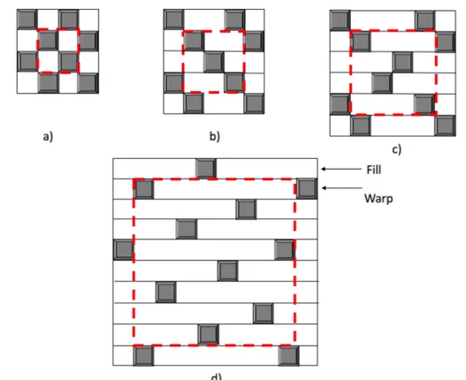
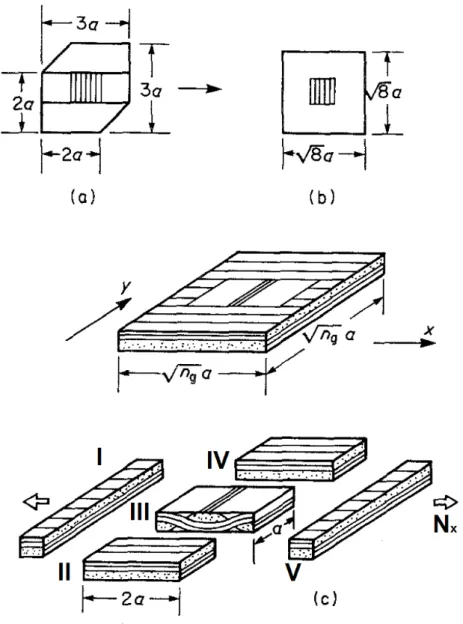
with ng ≥ 4 and where the interlaced regions are not connected are known as satin weaves. As defined by their ngvalues, the fabrics in Figure 2.5 are termed plain weave (ng= 2), twill
weave (ng= 3), 4 harness satin (ng= 4), and 8 harness satin (ng= 8) [43] The theoretical
Fig. 2.5 Examples of woven fabric patterns: (a) plain weave (ng= 2); (b) twill weave (ng= 3);
(c) 4-harness satin (ng= 4) and (d) 8-harness satin (ng= 8).
basis of the present analysis is the classical laminated plate theory. Under the assumptions of the Kirchhoff hypothesis, the constitutive equations are expressed in the condensed form as:
( N M ) = " A B B D # ( ε0 k ) (2.4) N and M are membrane stress resultants and moment resultants, respectively; epsilon0 an k are the strain and curvature of the laminate geometric mid-plane, respectively. The components of the stiffness matrices A,B and D are evaluates as follows:
(Ai j, Bi j, Di j) = n
∑
k=1 Z hk−1 hk (Qi j)k(1, z, z2)dz (i, j = 1, 2, 6) (2.5) where the reduced sirens constants Qi j corresponding to the lamina defined by hkand hk−1in the thickness direction are used in the calculations. The subscript 1,2 and 6 indicate in xyz coordinate system, the x direction, the y direction , and the x-y plane, respectively. More
2.7 Modeling of woven fabrics 23 explicitly last equation can be written as:
Ai j= n
∑
k=1 (Qi j)k(hk− hk−1) (2.6) Bi j= 1 2 n∑
k=1 (Qi j)k(hk2− hk−12) (2.7) Ci j =1 3 n∑
k=1 (Qi j)k(hk3− hk−13) (2.8)The inverted form is given by: ( ε0 k ) = " A′ B′ B′ D′ # ( N M ) (2.9) When the effect of temperature change is taken into account the constitutive relation and should be written as:
( N M ) = " A B B D # ( ε0 k ) − ∆T ( e A e B ) (2.10) where: e Ax e Ay e Axy = n
∑
k=1 Z hk−1 hk Q11 Q12 Q16 Q12 Q22 Q26 Q16 Q26 Q66 k αxx αyy αxy k dz (2.11) e Bx e By e Bxy = n∑
k=1 Z hk−1 hk Q11 Q12 Q16 Q12 Q22 Q26 Q16 Q26 Q66 k αxx αyy αxy k zdz (2.12) ∆T indicates a small uniform temperature change and α denotes the thermal expansion coefficients. The inverted form is given by:( ε0 k ) = " A′ B′ B′ D′ # ( N M ) + ∆T ( e A′ e B′ ) (2.13) where: ( e A′ e B′ ) = " A′ B′ B′ D′ # ( e A e B ) (2.14) The constants eA′and eB′represent respectively , the in-plane thermal expansion and thermal bending coefficients. Based upon the iso-stress and iso-strain assumptions, the above con-stitutive equations can be used to obtain the bounds of the thermoelastic properties. The
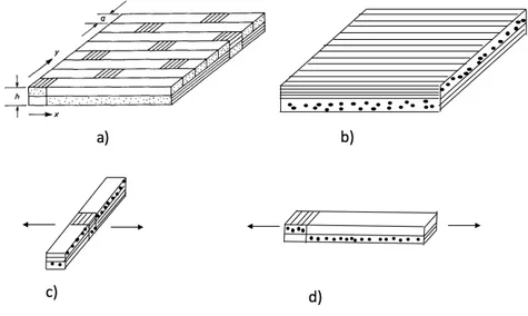
upper bounds of compliance constants are obtained by inverting the compliance constant matrix. Similarly, the upper bounds of stiffness constant are derived from the iso-strain assumption; the lower bounds of compliance constants are then obtained by inverting the stiffness constant matrix. Three techniques for modeling the stiffness and strength properties of fabric composites. Ishikawa and Chou developed three analytical models to predict the stiffness and coefficient of thermal expansion of woven fabric composites. [1] These are the mosaic model, the crimp model (fibre undulation model) and the combination of the above two, the bridging model. [62] The mosaic model described the fabric as an assemblage of asymmetrical cross-ply laminates with no fibre undulation and gave good predictions for fabrics with few interlaced regions, such as satin fabric. The crimp model accounted for the fibre undulation using shape functions was more suitable for plain weave composites. Finally, the bridging model was developed for satin woven fabrics in order to describe the difference in properties between the straight threads region and the interlaced regions.[1]
2.7.1
Mosaic Model
The basis of idealization of the “mosaic model” can be seen from Figure 2.6. The key simpli-fication of the mosaic model is the omission of the fiber continuity and crimp (undulation) that exist in an actual fabric. In general, a fabric composite idealized by the mosaic model can be regarded as an assemblage of pieces of asymmetric cross-ply laminates. Assuming
Fig. 2.6 The mosaic model:(a) repeating region in a eight-harness satin composite; (b) basic cross-ply laminate; (c) parallel model; (d) series model.
2.7 Modeling of woven fabrics 25 that fibers are aligned along the x direction, the stiffness constant, Qi j of a unidirectional
lamina, which has orthotropic symmetry in the x-y plane, are given by: Qi j= E11 Dv ν12E22 Dv 0 ν21E11 Dv E22 Dv 0 0 0 G12 (2.15) where Dv= 1 − ν12ν21 (2.16)
Here E11 and E22 are the Young’s moduli, G12is the in-plane shear modulus, and ν12denotes
the Poisson’s ratio relating the transverse strain in the x2direction and the applied strain in
the x1direction. The Qi j constants are symmetrical, i.e Qi j = Qji. The laminate is composed
of two unidirectional laminae of thickness h/2. The total laminate thickness is h and the x-y coordinate plane is positioned at the geometrical mid-plane of the laminate, k = 1 and k = 2 define, respectively, the laminae with fibers in the y and x directions. The non-vanishing stiffness constants are:
A11 = A22 = (E11+ E22)h 2Dv A12 =ν12E22h Dv A66 = G12h B11 = −B22 = (E11− E22)h2 8Dv D11 = D22 = (E11+ E22)h3 24Dv D12 =ν12E22h 3 12Dv D66 =G12h 3 12 (2.17)
The extension-bending coupling costants B11and B22do not vanish because E11 ̸= E22. Also,
it is understood that Ai j, Bi j and Di j are symmetrical constants.
Nxx Nyy Nxy = A11 A12 0 A12 A11 0 0 0 A66 ε0xx ε0yy ε0xy + B11 0 0 0 −B11 0 0 0 0 kxx kyy kxy (2.18)
Mxx Myy Mxy = B11 0 0 0 −B11 0 0 0 0 ε0xx ε0yy ε0xy + D11 D12 0 D12 D11 0 0 0 D66 kxx kyy kxy (2.19) Inverting previous equation the following are obtained:
ε0xx ε0yy ε0xy = A′11 A′12 0 A′12 A′11 0 0 0 A′66 Nxx Nyy Nxy + B′11 B′12 0 −B′12 −B′11 0 0 0 0 Mxx Myy Mxy (2.20) kxx kyy kxy = B′11 −B′12 0 −B′12 −B′11 0 0 0 0 Nxx Nyy Nxy + D′11 D′12 0 D′12 D′11 0 0 0 0 Mxx Myy Mxy (2.21) In the bound approach, the two-dimensional extent of the fabric composite plate is simplified by considering two one-dimensional models where the pieces of cross-ply laminates are either in parallel or in series. In the parallel model, a uniform state of strain ε0, and curvature k, in the laminate midplane is assumed as a first approximation. For the one dimesional repeating region of length nga, where a denotes the yarn width, an average membrane stress
Nx is defined as: Nx= 1 nga Z nga 0 Nxdy = 1 nga[ Z a 0 (A11ε0xx+ A12ε0yy+ B11kxx)dy + Z nga 0 (A11ε0xx+ A12ε0yy+ B11kxx)dy] = (A11ε0xx+ A12ε0yy) + 1 nga[aB T 11+ (nga− a)B L 11]kxx = A11ε0xx+ A12ε0yy+ (1 − 2 ng)B L 11kxx (2.22) The factor (1 −n2
g) appears because the terms B T
11for the interlaced region and non-interlaced
region BL11 have opposite signs, namely BT11=-BL11. Other average stress resultant can be written similar for uniform mid-plane strain, ε0and curvature k. The moment resultant Mx
for example is:
Mx= 1 nga Z nga 0 Mxdy = D11kxx+ D12kyy+ (1 − 2 ng)B L 11kxx (2.23)
![Fig. 2.1 Classification of composites based on matrix materials[6]](https://thumb-eu.123doks.com/thumbv2/123dokorg/2970071.27228/24.892.122.731.305.491/fig-classification-composites-based-matrix-materials.webp)
![Fig. 2.7 Fibre undulation model. [43]](https://thumb-eu.123doks.com/thumbv2/123dokorg/2970071.27228/46.892.253.628.502.873/fig-fibre-undulation-model.webp)
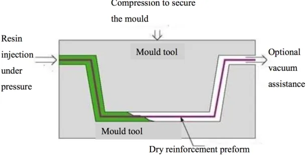
![Fig. 2.10 VARIM Process: (a) lay-up, (b) pre-filling, (c) filling, (d) post filling. [30]](https://thumb-eu.123doks.com/thumbv2/123dokorg/2970071.27228/55.892.136.784.167.433/fig-varim-process-lay-filling-filling-post-filling.webp)