Technical Report CoSBi 25/2007
A BetaWB model for the NF-κB pathway
Roberto Larcher
Cosbi, Trento, Italy
Dipartimento di Ingegneria e Scienza dell’informazione,
Unitversit`
a di Trento
[email protected]
Adaoha Ihekwaba
Cosbi, Trento, Italy
Dipartimento di Ingegneria e Scienza dell’informazione,
Unitversit`
a di Trento
[email protected]
Corrado Priami
Cosbi, Trento, Italy
Dipartimento di Ingegneria e Scienza dell’informazione,
Unitversit`
a di Trento
Second Level International Master in
Computational and Systems Biology
Master Thesis
A BetaWB model for the NF-κB
pathway
Advisor
Adaoha Ihekwaba
Co-advisor
Corrado Priami
Student
Roberto Larcher
Academic year 2006/2007
Contents
Introduction 1
1 ODE model of the NF-κB pathway 3 1.1 The NF-κB model . . . . 3 2 From determinism to stochasticity 7 2.1 Nucleus and cytoplasm volumes . . . 7 2.2 From concentrations to molecules numbers . . . 9 2.3 Deterministic rate constants translation . . . 9 3 The BetaWB abstraction 11 3.1 Identifying and defining BetaWB bio-processes . . . 11 3.2 The IκBα molecule . . . . 11 3.3 Creating new molecules . . . 17
4 Results 19
5 Conclusions and further work 21 A The BetaWB model of the NF-κB pathway 25
Acknowledgments 39
Introduction
NF-κB (Nuclear Factor-kappa B) is a protein complex which is a transcription factor. NF-κB is found in many cell types and is involved in cellular responses to stimuli such as stress, cytokines, free radicals, ultraviolet irradiation, and bacterial or viral antigens [1]. NF-κB plays a key role in regulating the immune response to infection. Consistent with this role, incorrect regulation of NF-κB has been linked to cancer, inflammatory and autoimmune diseases, septic shock, viral infection and improper immune development. NF-κB has also been implicated in processes of synaptic plasticity and memory [2].
This nuclear factor is a dimer composed by NF-κB proteins. In mammals they are a small group of proteins made up of five members: Rel (also known as c-Rel), RelA (also known as p65 and NF-κB3), RelB, NF-κB1(p50), and NF-κB (p52) [3]. All five proteins have a Rel homology domain (RHD) which serves in their dimerisation, in DNA binding, and is the main regulatory domain [4]. The RHD contains at its C-terminus a nuclear localisation sequence (NLS), which is rendered inactive through binding of specific NF-κB inhibitors, known as Inhibitor-κB (IκB) proteins [4].
The NF-κB is widely studied because it regulates numerous genes that play important roles in inter- and intra-cellular signalling, cellular stress responses, cell growth, survival and apoptosis. The specificity and temporal control of gene expression are of crucial physiological interest. For this reasons the understand-ing of the specific mechanisms that govern NF-κB-responsive gene expression is fundamental for the realisation of the potential of the NF-κB as drug target for many diseases (as chronic inflammatory and autoimmune diseases).
One of the instruments used to reach a better understanding in this field is the modelling. It is widely exploited to answer questions when experimental approach is impossible, difficult or too expensive to be employed. A model (that takes inspiration from the one described in [5]) is presented in [6], its aim is to get a better comprehension of the elements that regulate the NF-κB translocation from the cytoplasm to the nucleus. It does not consider all the NF-κBs but just its most common form, the p50-RelA dimer. As other NF-κB complexes, this dimer is sequestered in the cytoplasm by IκB family proteins (IκBα, IκBβ and IκBε). The phosphorylation-induced ubiquitination of IκBs leads to NF-κB activation and thus to its translocation in the nucleus. This phosphorylation depends on two protein complexes: the IκN kinase (IKK) complex end the E3IκB ubiquitin ligase complex (not considered in the model) [7]. Once
poly-ubiquitinated IκBs undergo rapid degradation through the 26S proteasome and the liberated NF-κB dimers translocate to the nucleus where they participate in transcriptional activation of specific target gene [3]. IκBα synthesis is controlled
2 CONTENTS
by a highly NF-κB-responsive promoter generating autoregulation of NF-κB signalling. In this model there are significant oscillations in the concentration of NF-κB in the nucleus. The paper [6] presents a model of the (TNF-α mediated) NF-κB signal transduction pathway, and uses sensitivity analysis to identify those parameters that exert the greatest control on the oscillatory concentrations of NF-κB in the nucleus.
The model presented in [6] is an ODE model. The aim of our work is to translate it in a BetaWB [8] model in order to verify that its behaviour does not change in the case of a stochastic approach. BetaWB is a framework for modelling and simulating biological precesses based on β-binders [9] and its stochastic extension [10].
Our work is also aimed at testing the correctness of the BetaWB framework. By now it has been used just to simulate simple biological examples and its employment to model the complicated NF-κB pathway is quite challenging.
The work is organised as follows. In the first chapter we introduce the ODE model our work is based on. Then we explain which are the fundamental steps to translate a model from deterministic to stochastic. In the fourth chapter we explain how we implemented the model in BetaWB. The last two chapters present results and conclusions of our work.
The original contribution of this work is the translation of the model from deterministic to stochastic and its implementation in BetaWB.
Chapter 1
ODE model of the NF-κB
pathway
The ODE model of the NF-κB pathway has been obtained using COPASI [11]. This tool takes as input the chemical reactions that take place in the pathway. It is necessary to specify the law that governs this reactions and their deterministic kinetic rate, than the tool automatically generates the ODE system that is used for simulations and various kind of analysis.
1.1
The NF-κB model
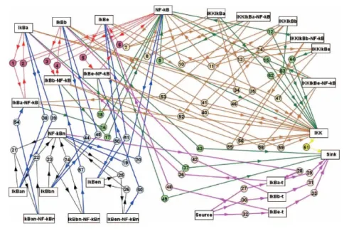
Figure 1.1 presents all the reactions that take place in the considered model. This depicts the IκB-NF-κB as described by Hoffmann [12] which seems to model the experimental data quite effectively. The supplementary information to the paper [12] gives all the relevant parameter.
This model, which is effectively the central signalling module of the NF-κB pathway, acts to transduce all the NF-κB response from the activation of IκB ki-nase (IKK) to the transport rates into and out of the nucleus of each of the com-ponents (IκBα/β/ε; NF-κB and derived complexes). IKK is represented here as a single entity (without separate descriptions for the IKKα/β heterodimer and its scaffold protein IKKγ. NF-κB heterodimer isoforms are also not specified in this model; this is because a single NF-κB isoform (p50/RelA) with tran-scriptional activation predominates in many cells [12]. Reactions were modelled as undirectional “primitives”, with the back reaction where appropriate being modelled as a separate undirectional reaction.
In the picture reactions are represented through arrows. Numbers on arrows are used as reference in Table 3 of [6] where there is a list of all the deterministic kinetic constants of the reactions. Different colours indicate different kind of reactions:
• Red: IκB-NF-κB cytoplasmic reactions • Blue: nuclear transports
• Black: nuclear reactions
4 Chapter 1. ODE model of the NF-κB pathway
Figure 1.1: Connection map of the ODE model
• Green: IκB phosphorylations and degradations • Brown: decomplexation reactions
• Yellow: IKK slow adaptation
An ordinal differential equation is specified for each molecule and complex. Two different differential equations are defined in the case of molecules that can reside both in the nucleus and in the cytoplasm. The Source and the Sink are two special species of the model. These two variables don’t represent a molecule but has been introduced to model the synthesis and the degradation of the other species.
All the species are presented in the following list: NF-κB the p50/p65 heterodimer in the cytoplasm.
IκBα/β/ε the three IκB isoforms considered in the model while are residing in the cytoplasm.
IKK the complex composed by the IKKα/β heterodimer and its scaffold pro-tein IKKγ in the cytoplasm.
IκBα/β/ε-NF-κB the complex composed by NF-κB and IκB isoforms and residing in the cytoplasm.
IKK-IκBα/β/ε The complex composed by IKK and IκB isoforms and resid-ing in the cytoplasm.
IKK-IκBα/β/ε-NF-κB The complex composed by IKK, IκB isoforms and NF-κB residing in the cytoplasm.
1.1. The NF-κB model 5
IκBα/β/ε-t mRNA molecule in the cytoplasm that codify for IκB isoforms. Molecule followed by an “n” Molecules that reside in the nucleus. Source It represents the genes codifying for the IκB isoforms mRNA. Sink All the degraded molecules.
All the reactions in the model follow the mass action law. Michaelis-Menten and similar approximations have not been used. This makes easer the trans-lation of this model in a stochastic one, therefore it is not necessary to look for missing deterministic kinetic constants, all the needed information can be obtained from the ODE model.
Chapter 2
From determinism to
stochasticity
The BetaWB model is a tool useful to model biological processes and run stochastic simulations. Therefore the first big difference between the ODE model and the BetaWB model is that the first one is deterministic instead the second one is stochastic. The translation from deterministic to stochastic implies two mandatory steps:
• Finding a reasonable volumes for compartments involved in the simulation. In deterministic models molecules quantities are expressed with concen-trations, therefore it’s not important to fix a simulation volume. On the other side stochastic simulation deals with number of molecules. This im-plies that we have to fix a volume for each compartment presents in the simulation in order to convert the molecules concentrations in numbers of molecules.
• Computing stochastic reaction rates.
Rate constants used in deterministic models can not be used in stochastic models as they are. They have to be converted in stochastic reaction rates. These reaction rates depend on more than one factor (kind of reaction, volume of the compartments where the reaction takes place,. . . ).
Obviously after these steps it is necessary to define a BetaWB program that models the pathway we are interested in.
2.1
Nucleus and cytoplasm volumes
When in the model it is present just one compartment its volume can be arbitrar-ily chosen. This is possible because in the ODE model there is no information to let us infer something about the volume.
However in our model there are two compartments, the nucleus and the cytoplasm. In this case the ODE model contains some information that has to be considered in order to define correct volumes. To make clear this concept we present a simple example where we have a molecule that can move from the
8 Chapter 2. From determinism to stochasticity
nucleus to the cytoplasm. The variable A indicates the number of molecule in the cytoplasm and the variable An indicates the number of molecules in the nucleus. The square brackets are used to indicate concentrations of molecules. The differential equations system that describe the evolution of this example is the following:
d[A]
dt = k1[An] d[An]
dt = −k2[An]
Now let us do some mathematical manipulations on these two equations. First of all we start with a conversion of the concentrations in number of molecules. To obtain this result it’s enough to divide the concentration by the volume where the molecule are resident (V1= nucleus volume,V2= cytoplasm volume) and by the Avogadro’s number (Na):
d A NAV1 dt = k1 An NAV2 d An NAV2 dt = −k2 An NAV2
After that, observing thatNA,V1andV2aret independent, we can modify the
first equation as follows:
1 NAV1 dA dt = k1 An NAV2 dA dt = V1 V2k1An
and we can do the same thing with the second equation:
1 NAV2 dAn dt = −k2 An NAV2 dAn dt = −k2An
Now, considering that we are dealing with molecules numbers, we can state that if one molecule is removed from the nucleus one molecule has to be put in the cytoplasm; and if one molecule is added to the cytoplasm exactly one molecule has to be removed from the nucleus. This leads by the fact that molecules can not be neither created nor destroyed. After this observation we can write this constraint:
dA dt = −
dAn
dt This observation implies the following:
k1An= V1 V2k2A n⇒ V1 V2 = k1 k2
After the achievement of this result we have to check which is the ratio between the “k1” and “k2” that are used in the ODE model we considered. In our case we have that k1 is equal to k2. This means that the two compartments have the same volumes.
Clarified this point, given that the ODE model suggests us just the ratio between the two volumes and not their dimensions, we decided to fix arbitrarily the diameter of our cell to 20 micrometre and to compute volumes as conse-quence of this choice. Therefore we set the nucleus and cytoplasm volume to 2.09e−12 litre.
2.2. From concentrations to molecules numbers 9
2.2
From concentrations to molecules numbers
After the computation of the compartments volumes we can translate the con-centrations of the ODE model in number of molecules.
m = cNAV
where m is the number of molecules, c is the concentration expressed in Mol, NA is the Avogadro’s number expressed in mol−1 and V is the volume where
the molecules are immersed expressed in litre. This kind of rule is followed for all the species except the Source one. In the ODE model there is a quantity of 1 µM of Source species. Our intent is to introduce just one object of kind Source in the model instead of 1261245 as suggests the formula we just presented, it is more intuitive in a stochastic simulation. As we’ll see in the following this choice introduces some complications in the translation of the deterministic rate constants in stochastic reaction rates.
2.3
Deterministic rate constants translation
This is one of the most important operations in the translation of a model. It is easy to introduce an error and if it involves a key rate the results obtained with the stochastic model will be totally different from the one obtained through the original deterministic model.
It is not possible to translate all the rates with the same approach. A distinction between different kinds of reactions has to be done. In our model there are four kinds of reactions:
First order: the easiest case: nothing to do. These are the rates of reactions that have just one reactant:
A → . . .
In this case the reaction rate is exactly the same of the rate constant. The volume has not to be considered as it has to in the following cases. In this category of reactions are also included that ones that describe movement of molecules from the nucleus to the cytoplasm and vice versa.
Second order: these rates are associated with bimolecular interactions (reac-tions that have two different reactants):
A + B → . . .
in this case the volume influences the translation as shown in the following formula:
r = k NAV
wherer is the rate of reaction expressed in mol−2s−1,k is the rate constant expressed inM−1s−1,NA is the Avogadro’s number expressed in mol−1
and V is the volume where the molecule are immersed expressed inl. Homodimerization: in this case the rate refers to a reaction that involves two
molecules of the same kind as reactants: A + A → . . .
10 Chapter 2. From determinism to stochasticity
the formula suitable for this reaction is very similar to the previous one: r = 2k
NAV
Involving source object: these rates are associated with reactions that in-volve the source object. All these reactions in the ODE model are reac-tions of the first order:
source → source + . . .
but as explained in section 2.2 we treat the source object in a “special” way. In our model we insert just one of this object instead of 1261245. This implies that to obtain the same results obtained with the ode model we have to apply the following formula instead the standard first order reactions formula:
r = 1261245k
We has been facilitated in the translation by the fact that in the ODE model all the elementary reactions have been defined. The usage of approximations as the Michaelis-Menten equation has been avoided.
Chapter 3
The BetaWB abstraction
The ODE approach represents each species with a differential equation. From a theoretical point of view there are not differences between a protein and a pro-tein complex composed by two or more basic elements. Also, the same propro-tein in two different compartments is considered as two different species. Depending on the reactants and the products of the reactions (and on the molecules move-ment between compartmove-ments), negative and positive components are added to the equations. These equations are often automatically generated by tools as COPASI. Also in this tool the attention is focused on the reactions. As we will see in this section the BetaWB approach is totally different.
3.1
Identifying and defining BetaWB bio-processes
The BetaWB approach aims at identifying all the standalone molecules (not the complexes) and to represent them as bio-processes. Both the formation and the behaviour of the complexes are codified in the molecules that compose them.
All the elementary molecules in our model are represented by the follow-ing bio-processes: IκBα, IκBβ, IκBε, NF-κB, IKK, IκBα-t (it represents the mRNA of IκBα protein), IκBβ-t, IκBε-t and Source. Where each biological ele-ment is represented by the bio-process with the corresponding name and Source represents a fictitious process used to create new molecules.
These bio-processes are provided with interfaces to make possible the inter-actions that lead, for example, to complexes formation. Finally the pi-processes that delineate the behaviour of the bio-processes are defined; they have to rec-ognize in which state the bio-processes are and make the right set of actions possible. In the following sections we present the implementation of a bio-process, the one that represents the IκBα molecule. The purpose of this section is to explain the logic that has been followed in the code organization. The hole code of the model is reported in Appendix A.
3.2
The IκBα molecule
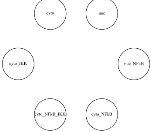
The first step in the “implementation” of a molecule consists in the identification of the states in which the molecule can be. Analysing the ODE model we realize that IκBα has six possible states; it can be:
12 Chapter 3. The BetaWB abstraction
• Free in the cytoplasm (cyto) • Free in the nucleus (nuc)
• Complexed to NF-κB in the cytoplasm (cyto NFkB)
• Complexed to NF-κB and IKK in the cytoplasm (cyto NFkB IKK) • Complexed to NF-κB in the nucleus (nuc NFkB)
• Complexed to IKK in the cytoplasm (cyto IKK)
According to this list all the possible states are shown in Figure 3.1. Given that
Figure 3.1: States in which IκBα can be
this molecule can interact with two proteins through two different binding sites, its bio-process has two interfaces:
• bind IKK to interact with the IKK bio-processes • bind NFkB to interact with the NF-κB bio-processes
To express the concept of compartmentalisation we exploit the idea presented in [13] where compartments are modelled through interface types. So interfaces that are exposed in different compartments have always incompatible types. Following this idea the types we associate with the IκBα bio-process interfaces are:
• bind IKK
– IkBa NFkB bind c → when the molecule is free in the cytoplasm – IkBa NFkB bind n → when the molecule is free in the nucleus – IkBaxIKK NFkB bind c → when the molecule is bound to IKK in
the cytoplasm • bind NFkB
3.2. The IκBα molecule 13
– IkBaxNFkB IKK bind c → when the molecule is bound to NF-κB in the nucleus
– IkBa IKK bind n → when the molecule is free in the nucleus – IkBaxNFkB IKK bind n → when the molecule is bound to NF-κB
in the nucleus
We specified in type file that all the types that finish with a different letter are incompatible.
After the states and interfaces identification, the next step is to build a π-process that pilots and recognizes state changes. First of all we define a channel for each possible state and set their rates to infinite:
<< cyto:inf, nuc:inf, cyto_NFkB:inf, cyto_NFkB_IKK:inf, nuc_NFkB:inf, cyto_IKK:inf, >>
Then we define a process composed by six processes in parallel: let proc_IkBa : pproc =
//IkBa in the cytosol !cyto{}.actions_IkBa_cyto | //IkBa in the nucleus !nuc{}.actions_IkBa_nuc |
//IkBa bound to NFkB in the cytosol !cyto_NFkB{}.actions_IkBa_cyto_NFkB | //IkBa bound to NFkB and IKK in the cytosol !cyto_NFkB_IKK{}.actions_IkBa_cyto_NFkB_IKK | //IkBa bound to NFkB in the nucleus
!nuc_NFkB{}.actions_IkBa_nuc_NFkB | //IkBa bound to IKK in the cytosol !cyto_IKK{}.actions_IkBa_cyto_IKK;
Each process has as guard a bang operation on a channel associated with one of the possible states. For all the parallelized processes after the bang operation a process follows, this process define the behaviour of the entire bio-process in a given state. For example the process actions IkBa cyto that follows the bang operation !cyto specifies the behaviour of the bio-process when it is in the state labelled with “cyto”.
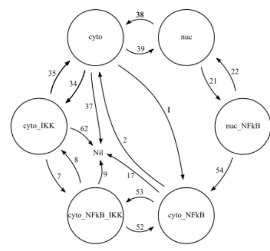
In order to define the processes we used in the previous BetaWB code we identify all the possible state changes that are permitted in the ODE model. These state changes are shown in Figure 3.2. A number is associated with each state change, it indicates the reaction (shown in Figure 1.1) we intend to model with that state change.
In the next lines we report the definitions of two pi-processes. The first process describes the actions that can be performed by the molecule when it is free in the cytoplasm. This is the first process:
14 Chapter 3. The BetaWB abstraction
Figure 3.2: Possible state changes. Numbers on arrows refer to the num-bering used in presenting reactions in Figure 1.1
//IkBa in the cytosol
let actions_IkBa_cyto : pproc =
(ch(3e-4,bind_NFkB,IkBa_NFkB_bind_n). //39 ch(bind_IKK,IkBa_IKK_bind_n).nuc<x>.nil + bind_NFkB<x>.ch(bind_IKK,IkBaxNFkB_IKK_bind_c). // 1 cyto_NFkB<x>.nil + bind_IKK{}.ch(bind_NFkB,IkBaxIKK_NFkB_bind_c). //34 cyto_IKK<x>.nil + die(1.13e-4)); //37
The process actions IkBa cyto is composed by four subprocesses composed by choice operators. This means that in this state we can alternatively perform four different actions. Each subprocess is a sequence of commands followed by a communication except for the last subprocess. The role of the communication is to implement the state change. It activates one of the guarded pi-processes in the IkBa proc process.
The last subprocesses does not have any communication as last command because its execution cause the bio-process death. A detailed description of the four subprocesses follows.
• ch(3e-4,bind_NFkB,IkBa_NFkB_bind_n). ch(bind_IKK,IkBa_IKK_bind_n).nuc<x>.nil
It models the reaction labelled with 39 in Figure 1.1: the movement of the IκBα molecule from the cytoplasm to the nucleus.
The two consecutive ch operations make the interfaces incompatible with the interfaces exposed in the cytoplasm and compatible with the interfaces exposed in the nucleus. These two operations are enough to model the movement of the molecule from the cytoplasm to the nucleus. After that the nuc<x> communication fires the change of state by activating the set of actions that can be performed by the molecule when it is free in the nucleus.
3.2. The IκBα molecule 15
cyto_NFkB<x>.nil
It models the reaction labelled with 1 in Figure 1.1 the IκBα complexation with NF-κB.
The communication bind NFkB<x> is possible only when the bind NFkB interface is complexed with another interface. Given that this interface is compatible only with the NF-κB molecule interface, this action is used to recognize the NF-κB binding. After the binding there is a ch operation to change the type of the bind IKK interface so that IκBα can complex with NF-κB and it changes its affinity with IKK molecules. The second operation is the communication cyto NFkB<x>. It change the state, acti-vating the pi-process that has the set of actions necessary to manage the IκBα bio-process when it is bounded to a NF-κB bio-process.
• bind_IKK{}.ch(bind_NFkB,IkBaxIKK_NFkB_bind_c). cyto_IKK<x>.nil
It models the reaction labelled with 34 in Figure 1.1: the IκBα complex-ation with IKK.
The set of actions executed is very similar to the one presented in the previous case.
• die(1.13e-4)
It models the reaction labelled with 37 in Figure 1.1: the IκBα degrada-tion.
This subprocess is very easy to understand, it just commands the bio-process death.
The second process that we consider describes the possible actions when the molecule is in the cytoplasm and is bound to NF-κB. When IκBα is in this state, it is complexed with NF-κB and can execute three actions:
let actions_IkBa_cyto_NFkB : pproc = (hide(bind_NFkB).unhide(bind_NFkB). ch(bind_IKK,IkBa_IKK_bind_c).cyto<x>.nil + // 2 bind_IKK{}.ch(bind_NFkB,IkBaxIKK_NFkB_bind_c). cyto_NFkB_IKK<x> + //53 @(2.25e-5).bind_NFkB<x>. ch(bind_NFkB,Destroyed).hide(bind_NFkB).die); //17
A detailed description of the subprocesses that are composed by the choice operator:
• hide(bind_NFkB).unhide(bind_NFkB). ch(bind_IKK,IkBa_IKK_bind_c).cyto<x>.nil
It models the reaction labelled with 2 in Figure 1.1: the unbinding of the NF-κB molecule.
The two consecutive operations hide and unhide are used to recognize the IκBα decomplexation from the NF-κB molecule. It works because the hide operation is permitted only on interfaces that are not complexed. The unhide operation is required to make again available the interface
16 Chapter 3. The BetaWB abstraction
because, after the decomplexation, the IκBα molecule is ready for other interactions. After this operation the pi-process executes a ch operation on the bind IKK interface because when IκBα decomplexes from NF-κB it changes its affinity with IKK molecules. As always the last operation is the communication that fires the state change.
• bind_IKK{}.ch(bind_NFkB,IkBaxIKK_NFkB_bind_c). cyto_NFkB_IKK<x>
It models the reaction labelled with 53 in Figure 1.1: the binding of the IKK molecule.
This reaction is modelled as all the binding reactions we have seen so far. • @(2.25e-5).bind_NFkB<x>.
ch(bind_NFkB,Destroyed).hide(bind_NFkB).die)
It models the reaction labelled with 17 in Figure 1.1: the degradation of the IκBα molecule.
This degradation can not be modelled simply with a die operation because in this case the IκBα is bounded to a NF-κB molecule. Before performing the die operation we have to be sure that IκBα is free in the nucleus, otherwise the operation destroys also the NF-κB molecule. To obtain an immediate decomplexation we execute a communication to inform the bounded NF-κB that IκBα is going to be degraded, than we perform a ch operation that changes the bind NFkB type to “Destroyed”. This special type has an infinite propensity for decomplexation with all the other types involved in the model. After this operation we execute a hide operation to be sure that the IκBα is not any more in a complexed status and then we destroy it through the die operation.
We now report with the definition of the bio-processes that represent the IκBα in its different states. As before we present just two examples; the bio-process that represents the IκBα free in the cytoplasm and the one that repre-sents the IκBα complexed with a NF-κB molecule in the cytoplasm. This is the first one:
let IkBa_cyto : bproc =
#(bind_NFkB:1,IkBa_NFkB_bind_c), #(bind_IKK:1,IkBa_IKK_bind_c) [actions_IkBa_cyto | proc_IkBa ];
It is quite immediate to define the correct bio-process. We have just to define the two interfaces, paying attention to the type we associate with them, and then put in the bio-process the set of action we defined for the state we are implementing (“cyto” in this case), plus, in parallel, all the guarded processes we have previously presented. This simplicity in the definition of the bio-process is due to the fact that we defined its internal pi-process in a structured way.
The second bio-process we report here is the one needed to represent a IκBα molecule complexed with a NF-κB molecule in the cytoplasm:
let IkBa_cyto_NFkB : bproc = #(bind_NFkB:1,IkBa_NFkB_bind_c), #(bind_IKK:1,IkBaxNFkB_IKK_bind_c) [actions_IkBa_cyto_NFkB | proc_IkBa];
3.3. Creating new molecules 17
We have again the two interfaces but in this casae we associate to the bind IKK interface a different type. This is due to the fact that the IκBα has two different affinities with IKK when it is free or bound with a NF-κB molecule. We followed the same logic as above to put in the bio-process the right pi-process.
All the molecules are present in the model has been modelled with the same technique, following the same principle.
3.3
Creating new molecules
In the presentation of the bio-process representing the IκBα molecule, we did not explain how we generate new molecules, therefore new bio-processes, in our abstraction. One of the molecule (it is not really a molecule) involved in generation processes is the Source. As we can see from the ODE model it is involved only in reactions like
Source → Source + IκBα-t
To implement this behaviour we decided to define a bio-process with a nil pi-process inside and a fake interface that we use just to recognize it in conditions associated to events. This is the definition of the process:
//mRNA source
let Source : bproc = #(Null:1,null) [ nil ];
To produce IκBα-t from this bio-process we added a split event to the model: //source produces ikBa mRNA
when (Source:9.71e-1) split(Source,IkBa_t);
The execution of this action has as result the consumption of a Source bio-process, and the production of a Source and a IkBa-t bio-process. The final balance is the production of aIkBa-t molecule. Note that after the split opera-tion the Source is immediately available for the creaopera-tion of other bio-processes.
Chapter 4
Results
The main results of our simulations are
• The steady state obtained running the model with a 0.1µM concentration of NF-κB and 1 Source bio-process.
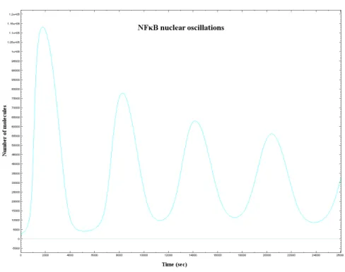
• The oscillatory behaviour obtained running the model with the steady state concentrations and adding 0.1µM of IKK molecules.
In both cases we obtained results that are nearly identical to the ones obtained with the ODE model. This is due to the fact that the oscillatory behaviour of the NF-κB is quite robust and to the fact that simulations involve big numbers of molecules therefore it is difficult that stochastic effects influence the system evolution.
In Figure 4.1 we have plotted the number of molecules of NF-κB against the time in an active cell (a cell that contains IKK molecules, thus TNF-α stimulated). There is an oscillation with a period of about ninety minutes, therefore the same kind of oscillation obtained in [5] and [6], the papers that describe the ODE model.
We tried to obtain the same results with a scaled system as well. With scaled system we mean a system where we put a number of molecules reduced of a factors. We keep fixed compartments volume and reduce the number of molecules. To obtain the same result we play with the rates. With this scaled system it is possible to have faster simulations, indeed a reduced number of participants implies that less reactions are fired during the simulations. However this increased velocity is paid with a decreased precision, indeed the system has a minor granularity.
The adjustment of the reaction rates has to be done keeping in mind which kind of reaction they are involved in. Another issue to consider is that it is possible that in the simulation there are molecule whose number can not be scaled. In our model this is the case of the Source molecule. We have just one bio-process of this kind, so we can not further reduce its presence in the simulation. Again to solve the problem we have to properly modify the rates involved in reactions that have the Source as reactant. Now we briefly show how it is necessary to manipulate the different kind of reaction rates:
First order: nothing to do.
20 Chapter 4. Results
Figure 4.1: NF-κB oscillations in the nucleus
Second order and homodimerization: multiply the original rate by the scal-ing factors.
Involving Source : dividing the original rate by the scaling factor s. Summarizing we obtain these results:
• A stochastic model for the NF-κB pathway.
• The possibility to scale the model in order to have faster simulations. • A comparison (that requires further analysis) between a stochastic and a
deterministic model.
Chapter 5
Conclusions and further
work
Our results show that BetaWB is suitable to model complex pathways, indeed, in the considered cases, our model behaves as the ODE model of [5]. If it is a good result on one side, on the other it seems to suggest that with this pathway a stochastic model is not needed: we obtain the same results of the ODE model but it takes more time to obtain them. However the fact that we obtained the same results in our case studies does not mean that all the case studies give the same results. For example performing sensitivity analysis with our stochastic model should be interesting; simulations that show regular oscillations with the ODE approach should behave in a totally different way in a stochastic context and it is possible also the opposite situation: stochastic effects should lead to oscillations that are not obtained with a deterministic approach [14].
Moreover, considering that stochasticity gives to interesting result with a low number of molecules, it should be interesting consider experiments with a small quantity of reacting molecules: for example a low concentration of transcription factor. It means a low probability of gene activation, however in case of binding of the NF-κB molecule with the DNA the size of mRNA’s burst is independent of the concentration. A model representing this behaviour should explain re-sults presented by Cheong et al. [15] and White. They found that average cell response, (measured as NF-κB nuclear translocation) is a decreasing function of TNF-α dose, across a very broad range of TNF-α concentrations, from 10 to 0.01ng/ml. However the single cell experiments performed by White’s group show that the individual cell response also decrease with the dose, but in ad-dition the fraction of cells that respond within a defined time period becomes smaller. Moreover, the experiment suggests that at very low dose, below 0.1 ng/ml, the single cell response is almost dose-independent and only the fraction of responding cells decrease with dose. This may suggest that stochastic cell activation following such a low dose stimulation is caused by erratic receptor activation caused by the limited number of TNF-α molecules.
Stochastic gene activation (leading to the burst of proteins) and stochastic cell activation (leading to the massive NF-κB nuclear translocation) provides a specific “stochastic robustness” in cell regulation. If a given gene is activated, a large burst of protein is produced, in order to assure a sufficient level of
22 Chapter 5. Conclusions and further work
activity of these proteins. Stochastic robustness assures the minimal response to the signal. Decreasing magnitude of the signal causes only lowering of the probability of response, which leads to a smaller fraction of responding cells. This can be a clever strategy: if the TNF-α signal is low, some cells respond by massive NF-κB translocation, whereas some do not respond at all. It helps to avoid ambiguity, such as when a small nuclear concentration of NF-κB lead to activation of an undefined fraction of NF-κB responsive genes. It is natural to expect that such undefined response might do more harm than good. Thus a better strategy at tissue level, with low signal, is to let some cell respond, and some cells ignore the signal. Stochastic robustness allows cells to respond differently to the same simulation, but make their individual responses better defined.
These observations leads to conclude that a stochastic approach could give interesting results. However, in order to reach them, our model needs several upgrades. First of all it is necessary to introduce a different mechanism to represent the gene activation. By now NF-κB molecules in the nucleus inter-act together and directly promote the production of IκBα mRNA. This is the reaction (number 28 in Figure 1.1) used to model the activation of the IκBα gene:
NF-κBn + NF-κBn → IκB-t
The DNA binding and the successive production of a burst of RNA molecules are not modelled loosing the possibility to exploit some of the benefits that we could have by using a stochastic approach.
In order to improve the model, we want also to critically analyse the imposed equality of the volumes assigned to the nucleus and the cytoplasm. As shown in section 2.1, from the differential equations involved in molecules translocation it is possible to conclude that in the ODE model presented in [6] the ratio between the cytoplasmic and nuclear volume is equal to one. The conclusion is strengthened by the fact that if we do not consider this constraint in the definition of the BetaWB model we obtain results that are discordant with deterministic ones. However we know that rarely, in a cell, the nucleus and the cytoplasm have comparable volumes, in the most of the cases the nucleus is considerable smaller than the cytoplasm. Modifying the model in order to respect this observation is not trivial. In fact if we reduce the dimension of the nucleus keeping constant the concentration of the molecules that it contains, we have to consider that its capacity to impact on the cytoplasmic molecules concentrations is reduced as well. This means that in order to reproduce the experimental results of [5] it is necessary to recalibrate the rates of the model taking this fact into account.
The technique used to implement the BetaWB model has a well defined structure (it is presented in chapter 3). There is a strong logic behind the criterion employed to identify the bio-processes and to define their pi-processes. This makes easy to modify the code and add new features. In order to verify this quality of extendability, we are planning to implement the p53 pathway and to add it to the current model. The p53 is regulated through a feedback loop involving its transcriptional target, mdm2. As it happen for the NF-κB, its concentration in cell compartments oscillates. This protein has a central role in many cancers and the interest on his behaviour is very high. The aim of our future work is to evaluate which are the effects of cross talks that take place
23
Appendix A
The BetaWB model of the
NF-κB pathway
//[steps = 1600, delta=150] //[steps = 2000, delta = 50] [steps = 1000, delta = 26] << EXPOSE:inf, HIDE:inf, UNHIDE:inf, CHANGE:inf, cyto:inf, nuc:inf, cyto_IkB:inf, nuc_IkB:inf, cyto_NFkB:inf, cyto_NFkB_IKK:inf, nuc_NFkB:inf, cyto_IKK:inf, x:inf >> //NFkB definition //NFkB actionslet action_NFkB_cyto : pproc = //NFkB in the cytosol
(ch(9e-2,bind_IkB,NFkB_IkB_bind_n).unhide(produce_IkBa_t). nuc<x>.nil +
bind_IkB{}.cyto_IkB<x>.nil); let action_NFkB_nuc : pproc = //NFkB in the nucleus
(ch(8e-5,bind_IkB,NFkB_IkB_bind_c).hide(produce_IkBa_t). cyto<x>.nil + //20-enter the cytosol
26 Chapter A. The BetaWB model of the NF-κB pathway
bind_IkB{}.hide(produce_IkBa_t).nuc_IkB<x>.nil + produce_IkBa_t{}.nuc<x>.nil +
produce_IkBa_t<x>.unhide(active).nil); let action_NFkB_cyto_IkB : pproc = //NFkB bound to IkB in the cytosol
(hide(bind_IkB).unhide(bind_IkB).cyto<x>.nil +
bind_IkB{}.hide(bind_IkB).unhide(bind_IkB).cyto<x>.nil); let action_NFkB_nuc_IkB : pproc =
//NFkB bound to ikB in the nucleus
(hide(bind_IkB).unhide(bind_IkB).unhide(produce_IkBa_t). nuc<x>.nil +
bind_IkB{}.ch(bind_IkB,NFkB_IkB_bind_c).cyto_IkB<x>.nil); //NFkB general process
let proc_NFkB : pproc = //NFkB in the cytosol !cyto{}.action_NFkB_cyto | //NFkB in the nucleus !nuc{}.action_NFkB_nuc |
//NFkB bound to IkB in the cytosol !cyto_IkB{}.action_NFkB_cyto_IkB | //NFkB bound to ikB in the nucleus !nuc_IkB{}.action_NFkB_nuc_IkB; //NFkB instances
//NFkB in the nucleus
let proc_NFkB_cyto : pproc = action_NFkB_cyto |
proc_NFkB;
//NFkB in the cytosol let proc_NFkB_nuc : pproc = action_NFkB_nuc |
proc_NFkB;
//NFkB bound to IkB in the cytosol let proc_NFkB_cyto_IkB : pproc = action_NFkB_cyto_IkB |
proc_NFkB;
//NFkB bound to ikB in the nucleus let proc_NFkB_nuc_IkB : pproc = action_NFkB_nuc_IkB |
proc_NFkB;
//IkBa definition //IkBa actions
let actions_IkBa_cyto : pproc = //IkBa in the cytosol
(ch(3e-4,bind_NFkB,IkBa_NFkB_bind_n). ch(bind_IKK,IkBa_IKK_bind_n).nuc<x>.nil + bind_NFkB<x>.ch(bind_IKK,IkBaxNFkB_IKK_bind_c).
27
cyto_NFkB<x>.nil +
bind_IKK{}.ch(bind_NFkB,IkBaxIKK_NFkB_bind_c). cyto_IKK<x>.nil +
die(1.13e-4));
let actions_IkBa_nuc : pproc = //IkBa in the nucleus
(ch(2e-4,bind_NFkB,IkBa_NFkB_bind_c). ch(bind_IKK,IkBa_IKK_bind_c).cyto<x>.nil + bind_NFkB<x>.ch(bind_IKK,IkBaxNFkB_IKK_bind_n). nuc_NFkB<x>.nil);
let actions_IkBa_cyto_NFkB : pproc = //IkBa bound to NFkB in the cytosol (hide(bind_NFkB).unhide(bind_NFkB). ch(bind_IKK,IkBa_IKK_bind_c).cyto<x>.nil + bind_IKK{}.ch(bind_NFkB,IkBaxIKK_NFkB_bind_c). cyto_NFkB_IKK<x> + @(2.25e-5).bind_NFkB<x>.ch(bind_NFkB,Destroyed). hide(bind_NFkB).die);
let actions_IkBa_cyto_NFkB_IKK : pproc = //IkBa bound to NFkB and IKK in the cytosol
(hide(bind_NFkB).unhide(bind_NFkB).ch(bind_IKK,IkBa_IKK_bind_c). cyto_IKK<x>.nil + hide(bind_IKK).unhide(bind_IKK).ch(bind_NFkB,IkBa_NFkB_bind_c). cyto_NFkB<x>.nil + @(2.04e-2).bind_IKK{}.ch(bind_IKK,Destroyed). ch(bind_NFkB,Destroyed). hide(bind_IKK).hide(bind_NFkB).die); let actions_IkBa_nuc_NFkB : pproc = //IkBa bound to NFkB in the nucleus
(hide(bind_NFkB).unhide(bind_NFkB).ch(bind_IKK,IkBa_IKK_bind_n). nuc<x>.nil +
@(1.38e-2).bind_NFkB<x>.ch(bind_NFkB,IkBa_NFkB_bind_c). ch(bind_IKK,IkBaxNFkB_IKK_bind_c).cyto_NFkB<x>.nil); let actions_IkBa_cyto_IKK : pproc =
//IkBa bound to IKK in the cytosol
(hide(bind_IKK).unhide(bind_IKK).ch(bind_NFkB,IkBa_NFkB_bind_c). cyto<x>.nil + bind_NFkB<x>.ch(bind_IKK,IkBaxNFkB_IKK_bind_c). cyto_NFkB_IKK<x>.nil+ @(4.07e-3).bind_IKK{}.ch(bind_IKK,Destroyed). hide(bind_IKK).hide(bind_NFkB).die);
//IkBa general process let proc_IkBa : pproc = //IkBa in the cytosol !cyto{}.actions_IkBa_cyto | //IkBa in the nucleus !nuc{}.actions_IkBa_nuc |
//IkBa bound to NFkB in the cytosol !cyto_NFkB{}.actions_IkBa_cyto_NFkB |
28 Chapter A. The BetaWB model of the NF-κB pathway
//IkBa bound to NFkB and IKK in the cytosol !cyto_NFkB_IKK{}.actions_IkBa_cyto_NFkB_IKK | //IkBa bound to NFkB in the nucleus
!nuc_NFkB{}.actions_IkBa_nuc_NFkB | //IkBa bound to IKK in the cytosol !cyto_IKK{}.actions_IkBa_cyto_IKK; //IkBa instances
//IkBa in the cytosol
let proc_IkBa_cyto : pproc = actions_IkBa_cyto |
proc_IkBa;
//IkBa in the nucleus let proc_IkBa_nuc : pproc = actions_IkBa_nuc |
proc_IkBa;
//IkBa bound to NFkB in the cytosol let proc_IkBa_cyto_NFkB : pproc = actions_IkBa_cyto_NFkB |
proc_IkBa;
//IkBa bound to NFkB and IKK in the cytosol let proc_IkBa_cyto_NFkB_IKK : pproc = actions_IkBa_cyto_NFkB_IKK |
proc_IkBa;
//IkBa bound to NFkB in the nucleus let proc_IkBa_nuc_NFkB : pproc = actions_IkBa_nuc_NFkB |
proc_IkBa;
//IkBa bound to IKK in the cytosol let proc_IkBa_cyto_IKK : pproc = actions_IkBa_cyto_IKK |
proc_IkBa;
//IkBb definition //IkBb actions
let actions_IkBb_cyto : pproc = //IkBb in the cytosol
(ch(1.5e-4,bind_NFkB,IkBb_NFkB_bind_n). ch(bind_IKK,IkBb_IKK_bind_n).nuc<x>.nil + bind_NFkB<x>.ch(bind_IKK,IkBbxNFkB_IKK_bind_c). cyto_NFkB<x>.nil bind_IKK{}.ch(bind_NFkB,IkBbxIKK_NFkB_bind_c).cyto_IKK<x>.nil + die(1.13e-4));
//IkBb in the nucleus
let actions_IkBb_nuc : pproc =
(ch(1e-4,bind_NFkB,IkBb_NFkB_bind_c).ch(bind_IKK,IkBb_IKK_bind_c). cyto<x>.nil +
29
//IkBb bound to NFkB in the cytosol let actions_IkBb_cyto_NFkB : pproc =
(hide(bind_NFkB).unhide(bind_NFkB).ch(bind_IKK,IkBb_IKK_bind_c). cyto<x>.nil + bind_IKK{}.ch(bind_NFkB,IkBbxIKK_NFkB_bind_c).cyto_NFkB_IKK<x>. nil + @(2.25e-5).bind_NFkB<x>.ch(bind_NFkB,Destroyed). hide(bind_NFkB).die);
//IkBb bound to NFkB and IKK in the cytosol let actions_IkBb_cyto_NFkB_IKK : pproc = (hide(bind_NFkB).unhide(bind_NFkB). ch(bind_IKK,IkBb_IKK_bind_c).cyto_IKK<x>.nil + hide(bind_IKK).unhide(bind_IKK). ch(bind_NFkB,IkBb_NFkB_bind_c).cyto_NFkB<x>.nil + @(7.5e-3).bind_IKK{}.ch(bind_IKK,Destroyed). ch(bind_NFkB,Destroyed).hide(bind_IKK).hide(bind_NFkB).die); //IkBb bound to NFkB in the nucleus
let actions_IkBb_nuc_NFkB : pproc =
(hide(bind_NFkB).unhide(bind_NFkB).ch(bind_IKK,IkBb_IKK_bind_n). nuc<x>.nil +
@(5.2e-3).bind_NFkB<x>.ch(bind_NFkB,IkBb_NFkB_bind_c). ch(bind_IKK,IkBbxNFkB_IKK_bind_c).cyto_NFkB<x>.nil); //IkBb bound to IKK in the cytosol
let actions_IkBb_cyto_IKK : pproc =
(hide(bind_IKK).unhide(bind_IKK).ch(bind_NFkB,IkBb_NFkB_bind_c). cyto<x>.nil + bind_NFkB<x>.ch(bind_IKK,IkBbxNFkB_IKK_bind_c). cyto_NFkB_IKK<x>.nil + @(1.5e-3).bind_IKK{}.ch(bind_IKK,Destroyed).hide(bind_IKK). hide(bind_NFkB).die);
//IkBb general process let proc_IkBb : pproc = !cyto{}.actions_IkBb_cyto | //IkBb in the nucleus !nuc{}.actions_IkBb_nuc |
//IkBb bound to NFkB in the cytosol !cyto_NFkB{}.actions_IkBb_cyto_NFkB | //IkBb bound to NFkB and IKK in the cytosol !cyto_NFkB_IKK{}.actions_IkBb_cyto_NFkB_IKK | //IkBb bound to NFkB in the nucleus
!nuc_NFkB{}.actions_IkBb_nuc_NFkB | //IkBb bound to IKK in the cytosol !cyto_IKK{}.actions_IkBb_cyto_IKK; //IkBb istances
//IkBb in the cytosol
let proc_IkBb_cyto : pproc = actions_IkBb_cyto |
30 Chapter A. The BetaWB model of the NF-κB pathway
//IkBb in the nucleus let proc_IkBb_nuc : pproc = actions_IkBb_nuc |
proc_IkBb;
//IkBb bound to NFkB in the cytosol let proc_IkBb_cyto_NFkB : pproc = actions_IkBb_cyto_NFkB |
proc_IkBb;
//IkBb bound to NFkB and IKK in the cytosol let proc_IkBb_cyto_NFkB_IKK : pproc = actions_IkBb_cyto_NFkB_IKK |
proc_IkBb;
//IkBb bound to NFkB in the nucleus let proc_IkBb_nuc_NFkB : pproc = actions_IkBb_nuc_NFkB |
proc_IkBb;
//IkBb bound to IKK in the cytosol let proc_IkBb_cyto_IKK : pproc = actions_IkBb_cyto_IKK |
proc_IkBb;
//IkBe definition //IkBe actions
//IkBe in the cytosol
let actions_IkBe_cyto : pproc =
(ch(1.5e-4,bind_NFkB,IkBe_NFkB_bind_n). ch(bind_IKK,IkBe_IKK_bind_n).nuc<x>.nil + bind_NFkB<x>.ch(bind_IKK,IkBexNFkB_IKK_bind_c).cyto_NFkB<x>. nil + bind_IKK{}.ch(bind_NFkB,IkBexIKK_NFkB_bind_c).cyto_IKK<x>. nil + die(1.13e-4)); //IkBe in the nucleus
let actions_IkBe_nuc : pproc =
(ch(1e-4,bind_NFkB,IkBe_NFkB_bind_c). ch(bind_IKK,IkBe_IKK_bind_c).cyto<x>.nil + bind_NFkB<x>.ch(bind_IKK,IkBexNFkB_IKK_bind_n). nuc_NFkB<x>.nil);
//IkBe bound to NFkB in the cytosol let actions_IkBe_cyto_NFkB : pproc = (hide(bind_NFkB).unhide(bind_NFkB). ch(bind_IKK,IkBe_IKK_bind_c).cyto<x>.nil + bind_IKK{}.ch(bind_NFkB,IkBexIKK_NFkB_bind_c). cyto_NFkB_IKK<x> + @(2.25e-5).bind_NFkB<x>.ch(bind_NFkB,Destroyed). hide(bind_NFkB).die);
//IkBe bound to NFkB and IKK in the cytosol let actions_IkBe_cyto_NFkB_IKK : pproc =
31 (hide(bind_NFkB).unhide(bind_NFkB).ch(bind_IKK,IkBe_IKK_bind_c). cyto_IKK<x>.nil + hide(bind_IKK).unhide(bind_IKK).ch(bind_NFkB,IkBe_NFkB_bind_c). cyto_NFkB<x>.nil + @(1.1e-2).bind_IKK{}.ch(bind_IKK,Destroyed). ch(bind_NFkB,Destroyed).hide(bind_IKK).hide(bind_NFkB).die); //IkBe bound to NFkB in the nucleus
let actions_IkBe_nuc_NFkB : pproc =
(hide(bind_NFkB).unhide(bind_NFkB).ch(bind_IKK,IkBe_IKK_bind_n). nuc<x>.nil +
@(5.2e-3).bind_NFkB<x>.ch(bind_NFkB,IkBe_NFkB_bind_c). ch(bind_IKK,IkBexNFkB_IKK_bind_c).cyto_NFkB<x>.nil); //IkBe bound to IKK in the cytosol
let actions_IkBe_cyto_IKK : pproc =
(hide(bind_IKK).unhide(bind_IKK).ch(bind_NFkB,IkBe_NFkB_bind_c). cyto<x>.nil + bind_NFkB<x>.ch(bind_IKK,IkBexNFkB_IKK_bind_c). cyto_NFkB_IKK<x>.nil + @(2.2e-3).bind_IKK{}.ch(bind_IKK,Destroyed).hide(bind_IKK). hide(bind_NFkB).die);
//IkBe general process let proc_IkBe : pproc = //IkBe in the cytosol !cyto{}.actions_IkBe_cyto | //IkBe in the nucleus !nuc{}.actions_IkBe_nuc |
//IkBe bound to NFkB in the cytosol !cyto_NFkB{}.actions_IkBe_cyto_NFkB | //IkBe bound to NFkB and IKK in the cytosol !cyto_NFkB_IKK{}.actions_IkBe_cyto_NFkB_IKK | //IkBe bound to NFkB in the nucleus
!nuc_NFkB{}.actions_IkBe_nuc_NFkB | //IkBe bound to IKK in the cytosol !cyto_IKK{}.actions_IkBe_cyto_IKK; //IkBe istances
//IkBe in the cytosol
let proc_IkBe_cyto : pproc = actions_IkBe_cyto |
proc_IkBe;
//IkBe in the nucleus let proc_IkBe_nuc : pproc = actions_IkBe_nuc |
proc_IkBe;
//IkBe bound to NFkB in the cytosol let proc_IkBe_cyto_NFkB : pproc = actions_IkBe_cyto_NFkB |
proc_IkBe;
32 Chapter A. The BetaWB model of the NF-κB pathway
let proc_IkBe_cyto_NFkB_IKK : pproc = actions_IkBe_cyto_NFkB_IKK |
proc_IkBe;
//IkBe bound to NFkB in the nucleus let proc_IkBe_nuc_NFkB : pproc = actions_IkBe_nuc_NFkB |
proc_IkBe;
//IkBe bound to IKK in the cytosol let proc_IkBe_cyto_IKK : pproc = actions_IkBe_cyto_IKK |
proc_IkBe;
//IKK definition //IKK actions
//IKK in the cytosol
let actions_IKK_cyto : pproc = (bind_IkB<x>.cyto_IkB<x>.nil + die(1.2e-4));
//IKK bound to IkB
let actions_IKK_cyto_IkB : pproc =
(hide(bind_IkB).unhide(bind_IkB).cyto<x>.nil +
bind_IkB<x>.hide(bind_IkB).unhide(bind_IkB).cyto<x>.nil); //IKK general process
let proc_IKK : pproc = //IKK bound to IkB
!cyto{}.actions_IKK_cyto | //IKK bound to IkB
!cyto_IkB{}.actions_IKK_cyto_IkB; //IKK istances
//IKK in the cytosol
let proc_IKK_cyto : pproc = actions_IKK_cyto|
proc_IKK;
let proc_IKK_cyto_IkB : pproc = actions_IKK_cyto_IkB |
proc_IKK;
//Bioprocesses definitions //NFkB in the cutosol let NFkB_cyto : bproc =
#(bind_IkB:1,NFkB_IkB_bind_c), #h(produce_IkBa_t:0,com_NFkB_NFkB), #h(active:0,activate_translation) [ proc_NFkB_cyto ];
33
let NFkB_nuc : bproc =
#(bind_IkB:1,NFkB_IkB_bind_n), #(produce_IkBa_t:0,com_NFkB_NFkB), #h(active:0,activate_translation) [ proc_NFkB_nuc ];
//Active NFkB in the nucleus let NFkB_nuc_active : bproc = #(bind_IkB:1,NFkB_IkB_bind_n), #(produce_IkBa_t:0,com_NFkB_NFkB), #(active:0,activate_translation) [ proc_NFkB ];
//NFkB bound to IkB in the cytosol let NFkB_cyto_IkB : bproc =
#(bind_IkB:1,NFkB_IkB_bind_c), #h(produce_IkBa_t:0,com_NFkB_NFkB), #h(active:0,activate_translation) [ proc_NFkB_cyto_IkB ];
//NFkB bound to IkB in the nucleus let NFkB_nuc_IkB : bproc =
#(bind_IkB:1,NFkB_IkB_bind_n), #h(produce_IkBa_t:0,com_NFkB_NFkB), #h(active:0,activate_translation) [ proc_NFkB_nuc_IkB ];
//IkBa in the cytosol let IkBa_cyto : bproc =
#(bind_NFkB:1,IkBa_NFkB_bind_c), #(bind_IKK:1,IkBa_IKK_bind_c) [ proc_IkBa_cyto ];
//IkBa in the nucleus let IkBa_nuc : bproc =
#(bind_NFkB:1,IkBa_NFkB_bind_n), #(bind_IKK:1,IkBa_IKK_bind_n) [ proc_IkBa_nuc ];
//IkBa bound to NFkB in the cytosol let IkBa_cyto_NFkB : bproc =
#(bind_NFkB:1,IkBa_NFkB_bind_c), #(bind_IKK:1,IkBaxNFkB_IKK_bind_c) [ proc_IkBa_cyto_NFkB ];
//IkBa bound to NFkB in the nucleus let IkBa_nuc_NFkB : bproc =
#(bind_NFkB:1,IkBa_NFkB_bind_n), #(bind_IKK:1,IkBaxNFkB_IKK_bind_n) [ proc_IkBa_nuc_NFkB ];
//IkBa bound to IKK in the cytosol let IkBa_cyto_IKK : bproc =
#(bind_NFkB:1,IkBaxIKK_NFkB_bind_c), #(bind_IKK:1,IkBa_IKK_bind_c)
[ proc_IkBa_cyto_IKK ];
34 Chapter A. The BetaWB model of the NF-κB pathway
let IkBa_cyto_NFkB_IKK : bproc = #(bind_NFkB:1,IkBaxIKK_NFkB_bind_c), #(bind_IKK:1,IkBaxNFkB_IKK_bind_c) [ proc_IkBa_cyto_NFkB_IKK ];
//IkBb in the cytosol let IkBb_cyto : bproc =
#(bind_NFkB:1,IkBb_NFkB_bind_c), #(bind_IKK:1,IkBb_IKK_bind_c) [ proc_IkBb_cyto ];
//IkBb in the nucleus let IkBb_nuc : bproc =
#(bind_NFkB:1,IkBb_NFkB_bind_n), #(bind_IKK:1,IkBb_IKK_bind_n) [ proc_IkBb_nuc ];
//IkBb bound to NFkB in the cytosol let IkBb_cyto_NFkB : bproc =
#(bind_NFkB:1,IkBb_NFkB_bind_c), #(bind_IKK:1,IkBbxNFkB_IKK_bind_c) [ proc_IkBb_cyto_NFkB ];
//IkBb bound to NFkB in the nucleus let IkBb_nuc_NFkB : bproc =
#(bind_NFkB:1,IkBb_NFkB_bind_n), #(bind_IKK:1,IkBbxNFkB_IKK_bind_n) [ proc_IkBb_nuc_NFkB ];
//IkBb bound to IKK in the cytosol let IkBb_cyto_IKK : bproc =
#(bind_NFkB:1,IkBbxIKK_NFkB_bind_c), #(bind_IKK:1,IkBb_IKK_bind_c)
[ proc_IkBb_cyto_IKK ];
//IkBb bound to NFkB and IKK in the cytosol let IkBb_cyto_NFkB_IKK : bproc =
#(bind_NFkB:1,IkBbxIKK_NFkB_bind_c), #(bind_IKK:1,IkBbxNFkB_IKK_bind_c) [ proc_IkBb_cyto_NFkB_IKK ]; //IkBe in the cytosol
let IkBe_cyto : bproc =
#(bind_NFkB:1,IkBe_NFkB_bind_c), #(bind_IKK:1,IkBe_IKK_bind_c) [ proc_IkBe_cyto ];
//IkBe in the nucleus let IkBe_nuc : bproc =
#(bind_NFkB:1,IkBe_NFkB_bind_n), #(bind_IKK:1,IkBe_IKK_bind_n) [ proc_IkBe_nuc ];
//IkBe bound to NFkB in the cytosol let IkBe_cyto_NFkB : bproc =
35
#(bind_IKK:1,IkBexNFkB_IKK_bind_c) [ proc_IkBe_cyto_NFkB ];
//IkBe bound to NFkB in the nucleus let IkBe_nuc_NFkB : bproc =
#(bind_NFkB:1,IkBe_NFkB_bind_n), #(bind_IKK:1,IkBexNFkB_IKK_bind_n) [ proc_IkBe_nuc_NFkB ];
//IkBe bound to IKK in the cytosol let IkBe_cyto_IKK : bproc =
#(bind_NFkB:1,IkBexIKK_NFkB_bind_c), #(bind_IKK:1,IkBe_IKK_bind_c)
[ proc_IkBe_cyto_IKK ];
//IkBe bound to NFkB and IKK in the cytosol let IkBe_cyto_NFkB_IKK : bproc =
#(bind_NFkB:1,IkBexIKK_NFkB_bind_c), #(bind_IKK:1,IkBexNFkB_IKK_bind_c) [ proc_IkBe_cyto_NFkB_IKK ]; //IKK in the cytosol
let IKK_cyto : bproc = #(bind_IkB:1,IKK_IkB_bind_c) [ proc_IKK_cyto ];
//IKK bound to IkB in the cytosol let IKK_cyto_IkB : bproc =
#(bind_IkB:1,IKK_IkB_bind_c) [ proc_IKK_cyto_IkB ];
//IkBa mRNA
let IkBa_t : bproc = #h(Null:1,null2) [ die(2.8e-4) ]; //IkBb mRNA
let IkBb_t : bproc = #h(Null:1,null1) [ die(2.8e-4) ]; //IkBe mRNA
let IkBe_t : bproc = #h(Null:1,null3) [ die(2.8e-4) ]; //mRNA source
let Source : bproc = #(Null:1,null) [ nil ];
//molecules definition //NFkB-IkBa in the cytosol: let NFkB_IkBa_cyto : molecule = {
36 Chapter A. The BetaWB model of the NF-κB pathway
NFkB : NFkB_cyto_IkB = (bind_IkB); IkBa : IkBa_cyto_NFkB = (bind_NFkB); };
//NFkB-IkBa in the nucleus: let NFkB_IkBa_nuc : molecule = {
((NFkB, bind_IkB, IkBa, bind_NFkB)); NFkB : NFkB_nuc_IkB = (bind_IkB); IkBa : IkBa_nuc_NFkB = (bind_NFkB); };
//NFkB-IkBb in the cytosol: let NFkB_IkBb_cyto : molecule = {
((NFkB, bind_IkB, IkBb, bind_NFkB)); NFkB : NFkB_cyto_IkB = (bind_IkB); IkBb : IkBb_cyto_NFkB = (bind_NFkB); };
//NFkB-IkBb in the nucleus: let NFkB_IkBb_nuc : molecule = {
((NFkB, bind_IkB, IkBb, bind_NFkB)); NFkB : NFkB_nuc_IkB = (bind_IkB); IkBb : IkBb_nuc_NFkB = (bind_NFkB); };
//NFkB-IkBe in the cytosol: let NFkB_IkBe_cyto : molecule = {
((NFkB, bind_IkB, IkBe, bind_NFkB)); NFkB : NFkB_cyto_IkB = (bind_IkB); IkBe : IkBe_cyto_NFkB = (bind_NFkB); };
//NFkB-IkBe in the nucleus: let NFkB_IkBe_nuc : molecule = {
((NFkB, bind_IkB, IkBe, bind_NFkB)); NFkB : NFkB_nuc_IkB = (bind_IkB); IkBe : IkBe_nuc_NFkB = (bind_NFkB); };
//IkBa-IKK in the cytosol let IkBa_IKK_cyto : molecule = {
((IkBa, bind_IKK, IKK, bind_IkB)); IkBa : IkBa_cyto_IKK = (bind_IKK); IKK : IKK_cyto_IkB = (bind_IkB); };
//IkBb-IKK in the cytosol let IkBb_IKK_cyto : molecule = {
((IkBb, bind_IKK, IKK, bind_IkB)); IkBb : IkBb_cyto_IKK = (bind_IKK);
37
IKK : IKK_cyto_IkB = (bind_IkB); };
//IkBe-IKK in the cytosol let IkBe_IKK_cyto : molecule = {
((IkBe, bind_IKK, IKK, bind_IkB)); IkBe : IkBe_cyto_IKK = (bind_IKK); IKK : IKK_cyto_IkB = (bind_IkB); };
//NFkB-IkBa-IKK in the cytosol let NFkB_IkBa_IKK_cyto : molecule = {
((NFkB, bind_IkB, IkBa, bind_NFkB), (IkBa, bind_IKK, IKK, bind_IkB)); NFkB : NFkB_cyto_IkB = (bind_IkB);
IkBa : IkBa_cyto_NFkB_IKK = (bind_NFkB, bind_IKK); IKK: IKK_cyto_IkB = (bind_IkB);
};
//NFkB-IkBb-IKK in the cytosol let NFkB_IkBb_IKK_cyo : molecule = {
((NFkB, bind_IkB, IkBb, bind_NFkB), (IkBb, bind_IKK, IKK, bind_IkB)); NFkB : NFkB_cyto_IkB = (bind_IkB);
IkBb : IkBb_cyto_NFkB_IKK = (bind_NFkB, bind_IKK); IKK: IKK_cyto_IkB = (bind_IkB);
};
//NFkB-IkBe-IKK in the cytosol let NFkB_IkBe_IKK_cyto : molecule = {
((NFkB, bind_IkB, IkBe, bind_NFkB), (IkBe, bind_IKK, IKK, bind_IkB)); NFkB : NFkB_cyto_IkB = (bind_IkB);
IkBe : IkBe_cyto_NFkB_IKK = (bind_NFkB, bind_IKK); IKK: IKK_cyto_IkB = (bind_IkB);
};
//source produces ikBa mRNA
when (Source:1.94) split(Source,IkBa_t); //Source produces IkBb mRNA
when (Source:2.25e-1) split(Source,IkBb_t); //Source produces IkBe mRNA
when (Source:1.6e-1) split(Source,IkBe_t); //IkBa mRNA produces IkBa
when (IkBa_t:4.08e-3) split(IkBa_t,IkBa_cyto); //IkBa mRNA produces IkBb
when (IkBb_t:4.08e-3) split(IkBb_t,IkBb_cyto); //IkBa mRNA produces IkBe
38 Chapter A. The BetaWB model of the NF-κB pathway
when (IkBe_t:4.08e-3) split(IkBe_t,IkBe_cyto); //Active NFkB produce IkBa
when (NFkB_nuc_active:inf) split(IkBa_t,NFkB_nuc);
//run 240800 NFkB_cyto || 1 Source
run 239213 IkBa_cyto || 316 NFkB_cyto || 105103 NFkB_IkBa_cyto || 27287 IkBb_cyto || 10474 NFkB_IkBb_cyto || 19469 IkBe_cyto || 7463 NFkB_IkBe_cyto || 274 NFkB_nuc || 237868 IkBa_nuc || 1805 NFkB_IkBa_nuc || 20817 IkBb_nuc || 396 NFkB_IkBb_nuc || 14852 IkBe_nuc || 283 NFkB_IkBe_nuc || 6940 IkBa_t ||
Acknowledgments
I would like to thank Adaoha for her help in understanding the NF-κB pathway, she has constantly supported me on the biological side. I thank Alessandro, Lorenzo and Alida for their support in the implementation of the model and Paola and Orkun for their help in mathematical issues. I also thank Radu because, with Adaoha, he worked to make possible my Californian “holiday”. Finally I thank Corrado that has constantly monitored my work and tried make better my stunted English.
Bibliography
[1] Thoma D Gilmore. The Rel/NF-κB signal transduction pathway: intro-duction. Oncogene, 19(49):6842–6844, 1999.
[2] Albensi BS and Mattson MP. Evidence for the involvement of TNF and NF-kappaB in hippocampal synaptic plasticity. Synapse, 35(2):151–159, 2000.
[3] Michael Karin, Yumi Yamamoto, and Q.May Wang. The IKK NF-κB system: a treasure trove for drug development. Nature, 3(1):17–26, 2004. [4] Ghosh S, May MJ, and Kopp EB. NF-kappa B and Rel proteins:
evolu-tionarily conserved mediators of immune responses. Annu. Rev. Immunol., 16:225–260, 1998.
[5] Alexander Hoffmann, Andre Levchenko, Martin L. Scott, and David Bal-timore. The IκB−NFκ Signaling Module: Temporal Control and Selective Gene Activation. Science, 298(5596):1241–1254, 2002.
[6] A.E.C. Ihekwaba, D.S. Broomhead, R.L. Grimley, N. Benson, and D.B. Kell. Sensitivity analysis of parameters controlling oscillatory signalling in the nf-kappab pathway: the roles of ikk and ikappabalpha. Syst Biol (Stevenage), 1(1):93–103, 2004.
[7] Karin M and Ben-Neriah Y. Phosphorylation meets ubiquitination: the control of nf-κb activity. Annu. Rev. Immunol., 18:6680–6684, 2000. [8] Lorenzo Demmat´e, Corrado Priami, and Alessandro Romanel. BetaWB:
modelling and simulating biological processes. In SCSC 2007, pages 777– 784, 2007.
[9] Corrado Priami and Paola Quaglia. Beta binders for biological interactions. In CMSB, Lecture Notes in Computer Science, pages 20–33, 2004.
[10] P. Degano, D. Prandi, C. Priami, and P. Quaglia. Beta-binders for biolog-ical quantitative experiments. Electronic Notes in Theoretbiolog-ical Computer Science, 164(3):101–117, October 2006.
[11] Stefan Hoops, Sven Sahle, Ralph Gauges, Christine Lee, and al. COPASI−a COmplex PAthway SImulator. Bioinformatics, 22(24):3067–3074, 2006. [12] Hoffmann A, Levchenko, Scott ML, and Baltimore D. Iκb-nf-κb
signal-ing module: temporal control and selective gene activation, supplementary material. Science Magazine, 298(5596):1241–1245, 2002.
42 BIBLIOGRAPHY
[13] Corrado Priami and Paola Quaglia. Operational patterns in beta-binders. volume 1 of Lecture Notes in Computer Science, pages 50–65, 2005. [14] Ralf Steuer. Effects of stochasticity in models of the cell cycle: from
quantized cycle times to noise-induced oscillations. Theoretical Biology, 228(3):293–301, 2004.
[15] Raymond Cheong, Adriel Bergmann, Shannon L. Werner, Joshua Rega, Alexander Hoffmann, and Andre Levchenko. Transient IκB Kinase Activity Mediates Temporal NF-κB Dynamics in Response to a Wide Range of Tumor Necrosis Factor-α Doses Formula. J. Biol. Chem, 281(5):2945–2950, 2006.