A Basic Model of Optimal Tax Enforcement under Liquidity Constraints

(1)

Volume 40, Issue 2

A Basic Model of Optimal Tax Enforcement under Liquidity Constraints

Alejandro Esteller-Moré Universitat de Barcelona & IEB

Abstract

I design a basic model based on the role of the tax administration as a lender of last resort (Andreoni 1992). If the administration's sole concern is for tax revenues, then it is optimal for it to make taxpayers take an unfair gamble. However, if it also gives some weight to the taxpayers' welfare in its objective function and this is sufficiently large, the situation might be reversed so that the auditing probability is lower and the evasion rate is higher. Under decreasing absolute risk aversion preferences, optimal enforcement is counter-cyclical (that is, greater liquidity constraints imply a higher level of enforcement) unless the administration attaches a considerable amount of weight to taxpayers' utility, which – at least in “normal times” – seems implausible. These theoretical results are complemented with numerical simulations.

This study was supported by projects RTI2018-095983-B-I00 (MCIU/AEI/FEDER, UE) and 2017SGR796 (Generalitat de Catalunya)

Citation: Alejandro Esteller-Moré, (2020) ''A Basic Model of Optimal Tax Enforcement under Liquidity Constraints'', Economics Bulletin, Volume 40, Issue 2, pages 1707-1713

Contact: Alejandro Esteller-Moré - aesteller@ub.edu.

Submitted: May 10, 2020. Published: June 18, 2020.

(2)

1. Introduction

Does tax evasion vary along the economic cycle? This might be the case if taxpayers are liquidity constrained (Andreoni 1992). Under this scenario, the tax administration acting as a lender of last resort might be the only chance for taxpayers to smooth consumption along time, such that they are even willing to play an unfair gamble. We characterize optimal enforcement within this scenario.

This characterization depends on the objective function of the administration. If it only cares for the amount of revenue collected, it will play an unfair gamble with taxpayers, who will still evade. This situation holds unless the relative value attached to the marginal utility of taxpayers is enormous with respect to the value of revenue for the administration. Under DARA preferences and liquidity constrained taxpayers, enforcement is counter-cyclical1

; again, this could reverse under the unlikely situation previously referred. Hence, to some extent the administration plays a stabilization role under the threat of future severe inspections.

The structure of the rest of the paper is as follows: in Section 2, I characterize the behaviour of taxpayers under liquidity constraints; in Section 3, I obtain the optimal level of enforcement; in Section 4, numerical simulations are provided to exemplify those theoretical results; and Section 5 concludes.

2. Taxpayer’s Behaviour: Andreoni 1992

I follow Andreoni’s 1992 model. Homogeneous individuals live two periods, t = 1, 2. In t=1, they earn taxable income, �_!; the corresponding tax return might be audited in the future. In t=2, they get an untaxed bequest, �_"2

, which is known with certainty by individuals in t=1. Thus, the financial benefits from evasion accrue in t=1, while the costs of evasion – if audited – accrue in t=2. Apart from the traditional incentive to evade based on a fair gamble (i.e., the expected financial return from evasion is positive), this delay might create a peculiar financial incentive. This is due to a capital market imperfection because potential lenders do not know in advance about the existence of �_" (as taxpayers do), and so in absence of other collaterals, evasion is the only alternative I consider liquidity constrained individuals have to smooth consumption along time.

X1 is the amount of undeclared income in t=1 such that �_! = �_!− �_!#, where �_!# is the

reported amount of taxable income. Hence, consumption in t=1 is �_! = �_!− �_!#� = �' + ��!, where � is the personal income tax rate, and �' = �!(1 − �) is net income under full

compliance. Thus, evasion generates a virtual income equal to ��_!. With a random probability, �, the evader might be audited in t=2, and then consumption is �"$ = �"− (� + �)�!, where

� is the fine per unit of evaded taxes (Yitzhaki 1974), � ≡ � × �, F>1, and assume the interest rate is zero; otherwise, in absence of an audit, and with random probability (1 − �), �_"%$ = �".

1

Durán-Cabré et al. 2020 have empirically shown this is the case for Spain.

2

To simplify we assume this bequest is untaxed (or if taxed, there is no possibility of evasion). This is justified on the grounds that I just want to focus on the incentives to evade taxes (today) under the presence of liquidity constraints (today). I am not interested in dynamic models of evasion (Engel and Hines 1999; Niepelt 2005).

(3)

1

Intertemporal additively separable utility, U, is �(�_!) + (1 − �)�(�_"%$) + ��(�_"$), where u´´<0<u´3

. Therefore, ideally, the taxpayer would like to smooth consumption along time. I focus on financially constrained individuals, that is, �_" > �'. Andreoni 1992 showed that if �" is above a given threshold, that is, if taxpayers are severely financially constrained, they

might evade even if � < 0, where � ≡ � − �(� + �) is the expected profitability of cheating. To understand this, note that for �_! = 0, a positive optimal level of evasion holds if the FOC of the taxpayer’s intertemporal maximization problem with respect to �_!is positive, that is, �&_{(�')� − ��}&_(�

")(� + �)|'!() > 0 [1]

I define the marginal rate of substitution between current and future consumption, m, as � º �′(�!) �⁄ &(�"$), where � > 1 under liquidity constraints. Then, rearranging [1], we have:

� > �(1 − �) [2] Evading taxes (�_! > 0) is optimal if [2] holds. For a given tax rate, the right-hand side of [2], which is negative, will be larger in absolute levels, the larger the marginal rate of substitution, �. Hence, even for � < 0, those severely constrained (large �) will find evasion to be welfare-enhancing; that is, the benefit of smoothing consumption overcomes the cost of an unfair gamble (� < 0). This is the peculiar incentive of evasion under financial constraints. From total differentiation of the taxpayer’s FOC, *'!

*+ < 0, *'! *,! < 0 and *'! *,"> 0 4_{. Up to now, this is} standard.

3. Optimal Tax Enforcement: Basic Characterization

Given the optimal taxpayer’s behaviour, now I characterize the optimal enforcement policy, picked by the auditing probability. I consider a general objective function (see, e.g., Slemrod and Yitzhaki 1987):

{�!#� − �!�} + �{�(�!) + ��(�"$) + (1 − �)�(�"%$) − �} [3]

The aim of the administration is maximizing revenue collected5

, subject to achieving a minimum level of taxpayers’ welfare, R; V(.) is the taxpayer’s indirect utility function. Hence, if l=0, we are under the most common positive characterization of a tax administration; if l>0, the level of enforcement is chosen also taking into account taxpayers’ welfare. Analytically, l is the ratio between the marginal value of revenue collected due to increasing p and the social marginal utility for taxpayers of decreasing p. That is, due to a variation in p, the administration is indifferent between l more € for taxpayers and one more € of tax revenue collected. Conceptually, thus, l is the social taxpayer’s utility loss of increasing p.

The control variable of the above maximization problem is p, and the FOC is:

3

Partial derivates of functions of a single variable are indicated by a prime (as many primes, as the degree of the corresponding partial derivative).

4

The full derivation of these total derivatives is available upon request from the author.

5

(4)

F º C(� + �) − �-'!

-+D + �{�(�"

$_{) − �(�}

"%$)} = 0 [4]

Andreoni 1992 analysed the case where � = 0; if so, working on [4], we have: � = ./0#$!

#%

< 0 [5] Thus, under financial constraints, it is optimal for the administration to play an unfair gamble with taxpayers, and they will accept it if they are severely liquidity constrained (see eq. [2]). If � > 0, though, this is not necessarily so:

� = 123456"&')14(6"'9:/(./0) #$!

#%

[6]

In particular, given �(�_"%$) − �(�_"$) > 0, for a large value of l, it might be optimal for the administration to play a fair gamble with taxpayers, despite they are liquidity constrained. I will show this by means of numerical simulations.

Before that, I perform a basic comparative static analysis to see how enforcement reacts when the liquidity constraint situation varies. Totally differentiating [4], we get �� C*+

*,!D =

�� C-;

-,!D. This latter sign depends on the sign of −�

--,!I -'! -+J, where --,!I -'! -+J < 0 if

�′′′(�!)>0. The sign of this third derivative holds under Decreasing Absolute Risk Aversion

(DARA) preferences, which I assume from now on; it implies the degree of absolute prudence of the taxpayer,−�&&&(�_<) �⁄ (�&& _<), is positive and so absolute risk aversion is decreasing with wealth (see, e.g., Eeckhoudt et al. 2005, Section 1.5). All in all, if � < 0, *+

*,! < 0; so, if the

taxpayer becomes less financially constrained, enforcement will go down, that is, it is counter-cyclical. Results reverse if � > 0. I check this in Section 4.

4. Numerical Simulations

In accordance with DARA preferences, individual utility is logarithmic. Apart from this, throughout we assume W2=20, t=.5, and F=1.56. First of all, we characterize the taxpayer’s

behaviour. In Graph 1, we see that if the taxpayer is not liquidity constrained (W1=20), tax

evasion is null if µ<0, which is the case for p>.4, and as expected the lower the audit probability, the higher the evasion rate. Ceteris paribus, evasion is larger, the higher the level of liquidity constraint. For W1=5 (“75% constrained”), evasion is 100% even for µ<0, and it

only starts decreasing for p>.72. Hence, evasion soars in times of crisis. In Graph 2, we show how evasion varies for different levels of liquidity constraints and depending on the level of enforcement.

6

The aim of the numerical simulations is to compare across different performances of the administration (l_{) and different rates of liquidity constraints, rather than on the levels of enforcement or of evasion}

(5)

3

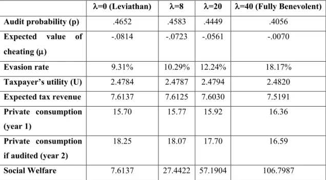
Regarding the administration, as expected enforcement decreases, the evasion rate increases, and the liquidity constraint is milder (check, e.g., the ratio between private consumption across periods) for larger values of l_{(Table 1). Here, the taxpayer is only “25% liquidity constrained”}

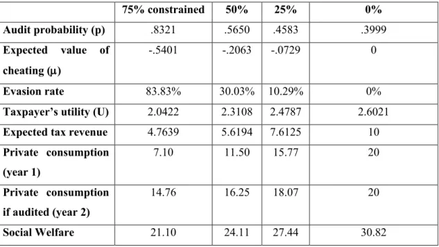
(15/20); that is why, even for l_=40,_µ_{<0. In the set of tables 2, though, we show that for large}

l and severely financially constrained individuals, µ>0 (first two columns of Table 2.3). Finally, in Graph 3, we show that tax enforcement is counter-cyclical unless the value of l_is

extremely large. In the absence of liquidity constraints, the optimal enforcement rate converges to .4, which is the situation for which µ=0. In fact, accordingly to what we saw in Section 3 pro-cyclicity only arises for µ>0, which Graph 4 shows.

0% constrained 25% constrained 50% constrained 75% constrained 0% 10% 20% 30% 40% 50% 60% 70% 80% 90% 100% 0. 00 0. 07 0. 14 0. 22 0. 29 0. 36 0. 43 0. 50 0. 58 0. 65 0. 72 0. 79 0. 86 0. 94 p=.01 p=.05 p=.2 p=.4 p=.6 p=.8 p=1 0% 10% 20% 30% 40% 50% 60% 70% 80% 90% 100% 90% 83% 76% 69% 62% 55% 48% 41% 34% 27% 20% 13% 6%

G_{raph 2.} _{Tax Evasion Evolution along} liquidity constraints rates for different levels of enforcement

G_{raph 1.}_{Tax Evasion Response to}

Enforcement for different levels of liquidity constraints

G_raph _3. _{Optimal enforcement rate} depending on the liquidity constraint rate and for different l

G_{raph 4.}_{Optimal expected value of cheating} depending on the liquidity constraint rate and for different l 0.35 0.40 0.45 0.50 0.55 0.60 50% 45% 40% 36% 33% 28% 25% 21% 19% 16% 13% 10% 5% 1% Lambda=0 Lambda=40 -0.240 -0.190 -0.140 -0.090 -0.040 0.010 50% 45% 40% 36% 33% 28% 25% 21% 19% 16% 13% 10% 5% 1% Lambda=40 Lambda=0

(6)

Table 1. _{Optimal Tax Enforcement for different weights of taxpayer’s utility (W}1=15)

l=0 (Leviathan) l=8 l=20 l=40 (Fully Benevolent)

Audit probability (p) .4652 .4583 .4449 .4056

Expected value of cheating (µ)

-.0814 -.0723 -.0561 -.0070

Evasion rate 9.31% 10.29% 12.24% 18.17%

Taxpayer’s utility (U) 2.4784 2.4787 2.4794 2.4820

Expected tax revenue 7.6137 7.6125 7.6030 7.5191

Private consumption (year 1) 15.70 15.77 15.92 16.36 Private consumption if audited (year 2) 18.25 18.07 17.70 16.59 Social Welfare 7.6137 27.4422 57.1904 106.7987

Table 2.1. _{Optimal Tax Enforcement for different liquidity constraint rates (}_l=0)

75% constrained 50% 25% 0% Audit probability (p) .9079 .5875 .4652 .3999 Expected value of cheating (µ) -.6349 -.2343 -.0814 0 Evasion rate 72.55% 26.78% 9.31% 0%

Expected tax revenue 4.8030 5.6275 7.6137 10

Private consumption (year 1) 6.81 11.34 15.70 20 Private consumption if audited (year 2) 15.47 16.65 18.25 20 Social Welfare 4.8030 5.6275 7.6137 10

(7)

5

75% constrained 50% 25% 0% Audit probability (p) .8321 .5650 .4583 .3999 Expected value of cheating (µ) -.5401 -.2063 -.0729 0 Evasion rate 83.83% 30.03% 10.29% 0%

Expected tax revenue 4.7639 5.6194 7.6125 10

Private consumption (year 1) 7.10 11.50 15.77 20 Private consumption if audited (year 2) 14.76 16.25 18.07 20 Social Welfare 21.10 24.11 27.44 30.82

75% constrained 50% 25% 0% Audit probability (p) 0 .36405 .4056 .3999 Expected value of cheating (µ) .4999 .0449 -.0070 0 Evasion rate 100% 63.92% 18.18% 0%

Expected tax revenue 0 4.7128 7.5190 10

Private consumption (year 1) 7.5 13.20 16.36 20 Private consumption if audited (year 2) 13.75 12.01 16.59 20 Social Welfare 87.04 98.35 106.80 114.08

(8)

5. Conclusions

Tax evasion and enforcement have traditionally been analysed within a static framework. However, the consideration of important shocks – for example, COVID-197

– may change some basic results. While there is a growing empirical literature on this, theoretical analyses are scarce. Here, I have shown that, unless fiscal and financial measures are enacted, taxpayers use evasion as a smoothing mechanism to mitigate the impact of liquidity constraints, under which the administration performs a counter-cyclical role, at least in “normal times” (see fn. (7)). That is, current evasion is certainly an unfair gamble for constrained individuals; and the more, the more binding liquidity constraints are.

References

Andreoni, J., (1992) “IRS as loan shark. Tax compliance with borrowing constraints” Journal of Public Economics 49, 35-46.

Durán-Cabré, J.M., A. Esteller-Moré, L. Salvadori (2020) “Cyclical Tax Enforcement” Economic Inquiry, forthcoming.

Eeckhoudt, L, C. Gollier, H. Schlesinger (2005) Economic and Financial Decisions under Risk, Princeton University Press: New Jersey.

Engel, E., J. R. Hines (1999) “Understanding Tax Evasion Dynamics”, NBER working paper number 6903.

Niepelt, D. (2005) “Timing tax evasion” Journal of Public Economics, 89, 1611-1637.

Slemrod, J., S. Yitzhaki (1987) “The optimal size of a tax collection agency” Scandinavian Journal of Economics, 89, 183-192.

Yitzhaki, S. (1974) “A Note on Income Tax Evasion: A Theoretical Analysis” Journal of Public Economics, 3, 201-2.

7