Biometrics parameters and fluxes estimation in Mediterranean mountainous grassland with remote sensing techniques

Abstract

European mountain grasslands, which include also Alps, Apennines and Pyrenees, are subject to relatively fast changes in both human activities and climatic conditions. Their role in the biogeochemical cycles is still highly uncertain and unknown and, in addition, the European Mediterranean mountain areas are unique and under-represented study cases. Therefore, their knowledge can therefore introduce new avenues in the understanding of the whole grassland ecosystem.

Remote sensing techniques appear as very useful tools in assessing and predicting productivity, quantity and quality of grassland over larger areas, whit higher temporal resolutions and lower cost than traditional methods of grassland sampling.

In this study we analyzed the biometric parameters of three different land uses of the Mediterranean grassland of Amplero (Abruzzo region, Italy): meadow (managed by harvesting and grazing that is the typical management in Amplero and in Appenines areas), natural (areas to exclude all external impacts) and pasture (used for animal grazing). Aim of this study has been the evaluation of the potentiality of remote sensing in the prediction or of biometric parameters, such as biomass and its partitioning, and LAI or Net Primary Productivity (NPP) and carbon fluxes (Net Ecosystem Exchange, NEE; Gross primary productivity, GPP) of a Mediterranean grassland. For this reason, we applied the following independent approaches: agronomic destructive sampling inventory, hyperspectral radiometric measurements, satellite images processing and micrometeorological methods.

We note that different management activities cause a broad variation in biomass dynamics. Cutting/harvesting and grazing have the same effects on the ecosystem reducing the quantity of available herbage and blocking the grassland growth. The effect of management on biomass quantity and quality can be detected by hyperspectral indexes and its relationships with investigated biometric parameters. Moreover, these relationships change also as consequence of growing vegetation phase and for this reason can be performed for analyzing the vegetation phenological status and characteristics of each type of managements present in the whole grassland area of Amplero. Finally, the estimation of GPP using radiometric methods it is possible to predict this variable both continuously and locally by CNR1 radiometer both discontinuously but on a larger area by MODIS images.

Riassunto

Le praterie montane europee, che includono il territorio delle Alpi, degli Appennini e dei Pirenei, sono soggette a cambiamenti relativamente veloci legati alle attività antropiche e alle condizioni climatiche. Il loro ruolo nei cicli biogeochimici è ancora molto incerto e poco conosciuto e, in più, esistono pochi casi di studio che riguardano le praterie montane mediterranee. Lo studio delle praterie mediterranee, dunque, potrebbe introdurre nuove informazioni sullo studio dell’intero ecosistema.

Le tecniche di telerilevamento consentono di ottenere informazioni sulla produttività, sulla qualità e sulla quantità delle coperture vegetali con un’ampia risoluzione spaziale e temporale ed a costi relativamente contenuti rispetto ai metodi tradizionali, basati sui rilievi di campo. In questo studio sono stati analizzati i parametric biometrici di tre differenti tipologie d’uso del suolo presenti nella prateria mediterranea di Amplero (Regione Abruzzo, Italia): meadow (sfalciato), natural (prateria indisturbata che non viene nè pascolata nè sfalciata) e pasture (pascolo) con l’obbiettivo di indagare le potenzialità del telerilevamento nel predire sia i parametri biometrici, come la biomassa, il contenuto di biomassa viva e morta e il LAI, sia la

micrometeorologico.

I risultati mostrano che i diversi utilizzi della prateria portano variazioni abbastanza ampie nella dinamica della biomassa della vegetazione. Il taglio, l’asportazione dell’erba e il pascolamento riducono la quantità di biomassa erbacea disponibile e bloccano la crescita della prateria. L’effetto dell’uso del suolo sulla quantità e qualità della biomassa può essere investigato utilizzando gli indici di vegetazione e le loro relazioni con i parametri biometrici misurati direttamente in campo. Queste relazioni, inoltre, sono strettamente legate alla fase di crescita della vegetazione e possono quindi essere utilizzate per analizzare lo stato fenologico della vegetazione e le caratteristiche della copertura vegetale dei diversi tipi di gestione presenti in tutta l’area di Amplero. Infine, utilizzando i metodi radiometrici è possibile predire il valore della GPP sia in maniera continua e locale con il radiometro CNR1 sia in maniera discontinua (per esempio ogni sedici giorni) ma su aree ampie con le immagini NDVI-MODIS.

D

S

’A

F

R

CORSO DI DOTTORATO DI RICERCA IN

ECOLOGIA

FORESTALE

–

XX

CICLO

BIOMETRIC PARAMETERS AND FLUXES ESTIMATION

IN MEDITERRANEAN MOUNTAINOUS GRASSLAND

WITH REMOTE SENSING TECHNIQUES

Settore Scientifico Disciplinare – AGR/05

Dottorando: Manuela Balzarolo

Firma

_________________________

Coordinatore: Prof. Paolo De Angelis

Firma

_____________________________

Tutore: Prof. Riccardo Valentini

Università degli Studi della Tuscia

Dipartimento di Scienze dell’Ambiente Forestale e delle sue Risorse (DISAFRI) Via S. Camillo de Lellis, snc 01100 Viterbo

Corso di Dottorato di Ricerca in Ecologia Forestale Coordinatore: Prof. Paolo De Angelis

Tesi di Dottorato di Ricerca in Ecologia Forestale (XX ciclo) di: Manuela Balzarolo

Index

SCIENTIFIC BACKGROUND OF THE STUDY... I GRASSLAND ECOSYSTEM AND REMOTE SENSING APPLICATIONS ... II MOTIVATIONS AND OBJECTIVES OF THE THESIS ... III

CHAPTER I ... 1

INTRODUCTION ... 1

1.1 MOUNTAINOUS MEDITERRANEAN GRASSLAND... 1

1.2 GRASSLAND CARBON STOCKS AND DISTRIBUTION INTO POOLS... 4

1.3 HYPERSPECTRAL PROXIMAL SENSING ... 4

1.4 NET PRIMARY PRODUCTIVITY OF GRASSLAND ... 6

1.5 FLUXES ESTIMATION AND REMOTE SENSING TECHNIQUES ... 8

1.6 THE STUDY AREA: AMPLERO SITE ... 10

1.6.1 Climate... 11

1.6.2 Grassland characteristics and management ... 13

CHAPTER II... 15

MATERIALS AND METHODS ... 15

2.1 SET-UP OF THE FIELD WORK... 15

2.2 BIOMETRIC MEASUREMENTS ... 16

2.3 ASSESSMENT OF NPP ... 17

2.3.1 Statistical analysis ... 19

2.4 HYPERSPECTRAL PROXIMAL SENSING: THE FIELDSPEC PRO® SPECTRORADIOMETER... 19

2.4.1 Radiometric sampling ... 19

2.4.2 Radiometric characterization of the study area ... 20

2.4.3 Data processing of the grass spectra ... 21

2.5 MODERATE-RESOLUTION IMAGING SPECTRORADIOMETER (MODIS) ... 23

2.5.1 MODIS data processing... 24

2.6 CONTINUOUS NDVI MEASUREMENTS BY CNR1 NET RADIOMETER... 25

Index

2.6.2 Data processing of CNR1 radiometer... 27

2.7 CONTINUOUS MEASUREMENTS OF FLUXES AT AMPLERO SITE ... 28

2.7.1 Theorical background ... 28

2.7.2 Eddy covariance system at Amplero site... 29

2.7.3 Data processing ... 30

Computing of carbon fluxes ... 30

Net Ecosystem Exchange... 31

Despiking and gapfilling ... 32

Fluxes partitioning ... 33

2.7.4 Meteorological sensors ... 33

CHAPTER III ... 34

RESULTS AND DISCUSSION ... 34

3.1 WEATHER CONDITIONS AND BIOMASS DYNAMICS... 34

3.2 NPP ASSESSMENT... 42

3.3 VARIATION IN REFLECTANCE SPECTRUM ... 46

3.4 COMPARING THE PERFORMANCE OF THE INDEXES IN ESTIMATING BIOMASS ... 48

3.5.1 Seasonal variability of NDVI, EVI and WBI ... 54

1.6.3 3.6 Biometric parameters and vegetation index relationship ... 55

3.6.1 Temporal variation ... 57

3.6.2 Spatial variation ... 61

3.7 PARTITIONING OF THE SOLAR RADIATION INTO THE WAVEBANDS OF CNR1... ... 63

3.8 NPP ESTIMATION FROM REMOTE DATA ... 66

3.9 CARBON DIOXIDE FLUXES OVER AMPLERO GRASSLAND ... 70

3.9.1 Evaluation of eddy measurements... 70

3.9.2 Carbon balance and correlated radiation fluxes ... 71

3.9.3 NEE and GPP estimation from NDVI... 75

CHAPTER IV ... 78

CONCLUSIONS ... 78

Scientific background of the study

During the last decades, becoming responsible of the observed global warming, greenhouse gases (GHGs) and their role in the global biogeochemical cycles changes have received a relevant institutional attention (IPCC, 2000).

Nowadays, the major challenge of the ecologists is to quantify the exchange of the radiatively active trace gases between ecosystems and atmosphere and to analyze how biotic, abiotic and anthropogenic factors control this exchange (Aubinet et al., 2000). Quantification and analysis of GHG exchange are necessary to understand not only the current exchange rates, but also to make hypothesis on the more probable effects of the climate and the land use changes and on the reactivity of several ecosystems.

Globally much interest has been given to forest ecosystems instead there are only few studies focused on the GHG budget at continental scale and less on the European grasslands. For this reason the potential contribute to the global warming of European grasslands is still highly uncertain.

Grassland ecosystems, as well as happens for all the other terrestrial ecosystems, contribute actively to these exchanges; they exchange CO2, N2O and CH4 between atmosphere, soil and

vegetation. Moreover the GHG fluxes of grasslands are strictly linked to their management (Soussana et al., 2007). The influence of the human activities on these exchanges is well described by analyzing the flux changes in response to the different grassland managements. N2O emitted by grassland soil is mainly due to the fertilization and animal waste system while

CH4 is produced by animals at grazing. Then the management strategies to reduce the GHG

emissions of grassland ecosystem must focus on the preservation of grasslands and on adaptation of their management in order to maintain their delicate equilibrium.

From an economical and political point of view the political administrations of many countries have established a framework of negotiations aimed at reducing GHGs and to combating the risks linked to the increase of CO2 and all GHG emissions displayed by the scientific

community. This forum started by the Conference of UN Environment (also known as "Earth Summit") Rio in 1992 and, at the end of the negotiations (Earth Summit in 1992; Berlin in 1995; Genève in 1996; Kyoto in 1997; La Haye in 2000 and Marrakesh in 2001), the terrestrial biosphere was considered in two sections (3.3 and 3.4 sections) of the Kyoto Protocol (available at www.unfccc.de). In particular, Section 3.3 refers to the assimilation of the sources and the sinks of GHGs “resulting from human activities directly related to land use change and forestry activities, limited to afforestation, reforestation and deforestation since 1990".

According with the Kyoto Protocol, the European Community decided to limit and reduce their emission of GHGs between 2008 and 2012 by 8% as compared to 1990 and issues related to land use, land-use change and forestry are be considered for Kyoto Protocol implementation (IPCC 2000). For this reason, significant information on the carbon sequestration of forest ecosystems across Europe (e.g. EU projects EUROFLUX, CANIF, MEDEFLU and the flux network CarboEurope) and of non-forest ecosystems (CARBOMONT and the grassland section of CarboEurope) now is available.

This study falls into the CARBOMONT project (EVK2-CT2001-00125) that aimed at the monitoring of the effects of land-use change on the carbon cycle of European mountain grasslands. For analyzing ecological, socio-economic and political background conditions at the European mountain scale, this project carried out in thirteen study sites of European member states, Switzerland and the Newly Associated States. In order to determine the effect of land use changes in these areas analyses carbon sequestration and flux partitioning in differently managed non-forest ecosystems (meadows, pastures, dwarf shrub communities and abandoned areas) was carried out. Moreover this project focus on the supporting the use of proximal and remotely sensed data for scaling-up the field data for assessing the spatial distribution of land cover, LAI, phenology status NPP and CO2 in the complex mountain grassland. The present

research activity takes place in the research of the connection between the vegetation characteristics and remote sensing applications.

Grassland ecosystem and remote sensing applications

Net primary production (NPP), the rate of biomass production per area, is an important attribute of the ecosystems (Asner et al., 2003, Paruelo et al., 1997). It determines, for instance, the total amount of energy available for upper trophic levels. In order to make decisions on animal movements among pastures, forage storage, stocking densities, etc., range managers need accurate estimates of biomass at the paddock level and at relatively detailed temporal resolution. Using classic agronomic methods the clipping must be conducted during the peak of pasture growth season and the sampling mast be effectuated o previously the same uncut area or on different area with the same vegetation composition and in the same ecological conditions. Therefore, these methods of grassland monitoring are limited by the small areas, number of samples, infrequent measurements and are also time-consuming and costly (Li et al., 1995). Remote sensing techniques appear as very useful tools in assessing and predicting changes in structure and functioning of ecosystems. Ground level remote sensing allows rapid evaluation of vegetation properties in a non-destructive way (Gamon et al., 1999, Mutanga et

al., 2004). Moreover, remote sensing technology from airborne and satellite platforms provide information of vegetation status and composition in large areas. Many high spectral resolution reflectance vegetation indices have been proposed with the aim of monitoring biomass, phenology and physiological conditions of plants and canopies (Peñuelas et al., 1998).

Few authors have applied remote sensing techniques to the problem of CO2 fluxes estimation in

grassland mountainous landscape. The remote sensing technologies could represent a new instrument available to ecologist and alpine-crops experts to support their chooses as recently exposed by several authors. Physical and physiological parameters of vegetation can be measured using particular instruments scheduled for the Earth Observation (EO) of remote sensing like radiometer (Hanna et al., 1999, Jakomulska et al., 2003). Mutanga et al. (2004) showed the possibility to make successful prediction of foliar quality using field spectroradiometry for the application of the approach using airborne sensors. The relationships based on plot-level measurements can be used to guide the development of larger, regional-scale models that would utilize satellite or aircraft data.

Whiting et al (Withing et al., 1992) demonstrated that Net Ecosystem Exchange (NEE) of CO2

flux at the tundra level could be predicted successfully using a spectral vegetation index, like NDVI (Normalized Difference Vegetation Index). Filella et al. (Filella et al., 2004) applied these techniques to Mediterranean shrubland affected by warming and drought and demonstrated that remote sensing approach is useful for assessment of seasonal and annual changes in biomass and CO2 uptake of this ecosystems.

Motivations and objectives of the thesis

In Europe grasslands cover more than 90 million ha of agricultural area that is about 22% of the EU-25 countries and represents an important economic and environmental resource; in Italy covers about 4.38 millions ha of the agricultural territory.

Grassland productivity is affected by fast changes due to anthropogenic activities and climatic conditions. Motivated by these changes in land management and climate, as well as the scarsity of long-term data on the carbon cycling in mountain grassland ecosystem, this study aims at quantifying the productivity and fluxes of a Mediterranean mountainous grassland. The location selected for the study was the grassland of Amplero (central Italy, Abruzzo Region) where activities were carried out over meadow (managed by harvesting and grazing that is the typical management in Amplero and in Appenines areas), natural (areas to exclude all external impacts) and pasture (used for animal grazing).

By means of different methodologies following specific aims are approached:

I. Assessment of net primary productivity of the different grassland landuses and its interaction with environmental conditions;

II. Estimation of grassland biometric parameters and productivity by remote sensing techniques at several spatial and temporal resolution at ground, tower and satellite levels;

III. Comparison of several radiometric sensors and definition of the most suitable sensor for estimating NDVI;

IV. Integration of eddy fluxes and remotely sensed data, collected at several temporal and spatial resolutions, by applying the correlation techniques.

Chapter I

Introduction

1.1 Mountainous Mediterranean grassland

The knowledge of grassland ecosystem dynamics is very important. As Soussana et al. suggest (Soussana et al., 2007), these ecosystems provide a variety of goods and services to support flora, fauna, and human populations worldwide.

Globally grasslands cover around 40 % of the ice-free terrestrial surface (White et al., 2000), but their role in the carbon cycle is currently poorly understood. This is mainly due to a less availability of data (Gilmanov et al., 2007) compared to the wide supply of flux measurements of forest ecosystems (Baldocchi et al., 2003). In addition, the European Mediterranean mountain areas are unique and under-represented study cases. The study of Mediterranean grassland can therefore introduce new avenues in the understanding of the whole ecosystem. European grasslands cover more than 40% (90 million ha) of agricultural area and about 22% of the EU-25 territory (EEA, 2005), representing an important economic and environmental resource. The share of grassland on the total Unit of Agricultural Area (UAA) ranges from 1% in Baleares (Spain) to almost 100% in the region of Valle d’Aosta (Italy), it is high in alpine regions and relatively low in Sweden and Finland (Figure 1). In Italy grasslands cover totally 28.17 % of UAA, consisting of 4.38 millions ha (Table 1).

The grassland landscape and its productivity are linked to several factors such as human activities (harvesting, fertilization and irrigation), animal grazing and environmental conditions (precipitation, drought and snow cover duration). Principally human activities as harvesting, mowing and grazing, in the European mountainous grassland influence grassland carbon budget impacting on CO2 plant assimilation and ecosystem respiration (Novick et al., 2004). The

removal of the above-ground plant mater by harvesting and grazing changes both soil temperature and moisture and, consequently, soil respiration. Fertilization changes available nutrients and the photosynthetic activities of plants, thus affecting the whole ecosystem respiration.

Chapter I - Introduction

Figure 1 - Share of grassland on total UAA (in %) (data from EEA, 2005) in the European Community

Table 1 - Distribution of grassland in some European countries (in 1000 ha and % on UAA). GRASSLAND Country in 1000 ha in % on UAA Finland 26.7 1.19 Greece 145.9 3.74 Denmark 186.4 6.97 Sweden 482.3 15.36 Italy 4378.9 28.17 Spain 7124.5 28.17 Germany 4969.6 29.28 France 9971.6 33.74 Portugal 1467.7 38.16 Belgium 536 38.49 Netherlands 891.9 45.75 Luxembourg 65 50.78 Austria 1917.4 56.84 UK 9905.8 60.58 Ireland 3193.4 73.04

Furthermore climatic conditions control the soil water availability and air humidity affecting CO2 assimilation in arid, semi-arid (Hastings et al., 2005) and temperate ecosystems (Baldocchi

et al., 1998, Novick et al., 2004). For instance, leaves stomatal conductance is reduced by low soil moisture. Through its effect on enzyme kinetics, temperature is another abiotic factor influencing the assimilation of CO2 in particular for high-latitude and high-elevation

ecosystems.

European mountain grasslands, which include also Alps, Apennines and Pyrenees, are subject to relatively fast changes in both human activities and climatic conditions. The carbon cycle in the sub-arctic mountain grasslands of Europe seems to be affected by climate changes more than local human impact (IPCC et al., 2000) while in the central European grasslands, also land management changes seem to affect the ecosystem structure and functionality (Cernusca et al., 1999). Considering the EU agricultural politic and financing, these changes will become more important in the early future.

The climate in the Mediterranean grasslands (South Italy, Spain and Portugal) falls into the Mediterranean climate. This climate extends predominantly from 32°N to 40°S latitude in both the northern and southern hemispheres, and covers the Mediterranean basin of Europe, north Africa and west Asia, southern Australia, the southwest coast of the United States, central Chile and the Cape region of south Africa (Nahal et al., 1981). The weather is characterized by warm/dry summers and mild/wet winters with rainfall occurring almost exclusively from November to February.

In the Mediterranean climate plant growth cycles depend on the rain distribution during the winter and the spring time (Xu et al., 2004). The absence of precipitation during summer season gives rise to a long drought period that may have a negative effect on carbon plant assimilation and productivity caused by a reduction of photosynthetic rates and leaf surface. In the last years, the frequency of both precipitation and drought changed dramatically in the whole Mediterranean basin. Two long term observations in the north-eastern inland of Spain and over the western Mediterranean confirmed this trend (Horcas et al., 2001). Moreover, little changes or even increases of the day/night temperature differences have been highlighted in the last 130 years: daily maximum temperatures have been increased at larger rates compared to daily minimum temperatures. This differential warming rate increased during the second half of the 20th century leading a several damages on productivity of ecosystems and consequent a reduction of economical opportunities offered by different agricultural areas.

Chapter I - Introduction

1.2 Grassland carbon stocks and distribution into pools

The importance of carbon pool assessment in terrestrial ecosystems is well known. Carbon stocks in the ecosystems are the key to understand the global carbon cycle. Generally, the long term carbon balance of grasslands has received little attention (Hui et al., 2006, Jones et al., 2004). Berninger et al. (2007, submitted) studied carbon balances and carbon stocks of 8 mountain grasslands eddy covariance sites and 22 sites with biomass data located in the European countries. Data used in this work were collected over a three-year period within the CARBOMONT project of the European Union 5th _{framework program (5FP). The carbon}

stocks in the analyzed grasslands were high and comparable to those of forest ecosystems, while carbon stocks in plant biomass is smaller (Berninger et al., 2007 submitted). The carbon accumulation in the grassland ecosystems occurs mostly below the ground (Soussana et al., 2004), where up to 98% of the total carbon stored can be sequestered in this compartment (Hungate et al., 1997). About two-thirds of terrestrial carbon is below the ground and this pool generally has much slower turnover rates than aboveground carbon (Schlesinger et al., 1977). Human activities, including harvesting of herbage, grazing and pasture management, influence the carbon stocks of grassland ecosystem. Therefore, the annual production of biomass in grassland can be large, but owing to the rapid turnover and the removals through the harvesting and grazing, the stock of aboveground biomass rarely exceeds a few ton per hectare. In addition, roots biomass and soil can accumulate large amounts of carbon but the detection of the changes of the stocks belowground is complicate. Mainly for such reason, methods based on flux measurements to assess carbon sequestrations of the grassland ecosystems are justified.

1.3 Hyperspectral proximal sensing

In the field of remote sensing the term “proximal” is used when the surface under investigation is few meters far from the detector or the spectrometer. In general proximal sensing techniques are used to validate remotely sensed data, as has been done in this study.

The term “hyperspectral” refers to those spectra made of a big number of narrow, continuously spaced spectral bands (Mutanga et al., 2004) and is a synonym of spectroscopy, spectroradiometry and rarely ultraspectral (Clark et al., 1999). Spectroscopy is a branch of physics concerned with the production, transmission, measurement and interpretation of electromagnetic radiation (Kumar et al., 2002). Spectrometry (or spectroradiometry) derives from spectro-photometry, the “measure” of photons as a function of wavelength. Instruments used in this field are named spectroradiometers and have the same characteristic of FielSpec HH PRO® _{(ASD, Boulder -CO), the spectroradiometer employed in the study.}

Ecological models and environmental studies require a wide range of input data, as well as data of biophysical vegetation characteristics, quality and quantity of biomass and its partitioning, leaf area index (LAI), and biochemical characteristics such as chlorophylls, carotenoids and nitrogen content. In addition to the strong necessity of high quality input data, available data from field observations are often inconsistent or totally absent. The low number of ground data necessary for both the initialization and the parameterization of models and the unknown uncertainty in their spatial distribution represent limiting factors for the application of ecological models at different scales and levels (local, regional or continental).

Quantitative remote sensing in a general, and imaging spectroscopy in a more deep level seem to be good techniques to fill the information gap explained before, to understand land-atmosphere carbon fluxes processes and to quantify and monitor plant photosynthesis needs of large areas and for long time periods (Field et al., 1993). Recent studies have also been shown that biochemical and biophysical properties of vegetation can be measured with a quantifiable uncertainty that can be incorporated in the land-biosphere models (Ustin et al., 2004a).

In general, the quantity of sun light that can be reflected or transmitted by leaves depends on biophysical plant properties such as the concentration of photosynthetic pigments (that capture sun light for photosynthesis), the water content, the dry plant matter and the leaf area index. During the growing season plant absorbs and reflects the solar light with different intensity. For instance, Rotondi et al.(2003) reported that the absorbance is reduced by pubescence, and that leaves appear more reflective after hairs have dried (Rotondi et al., 2003). Ustin et al. confirmed that reflectance and transmittance change in predictable directions following alterations of properties of xeromorphic plant leaves (Ustin et al., 2004a). In green leaves the photosynthetic pigments drive the light absorption in the visible (VIS, 400 - 700 nm) range of electromagnetic spectrum (Carter et al., 1991) where there is a minimum of the absorption at 550 nm. On the contrary, elements that compound dry leaves like cellulose, lignin and other structural carbohydrates play a fundamental role in reflecting radiation in the near-infrared (NIR, NIR, 700 - 1100 nm) region, where the absorption by biochemical parties is minimal. In this range, the internal structure of leaves and the numbers of pores for water and air affect the reflectance and the absorption made by photosynthetic pigments. Indeed, if intercellular air spaces and cell sizes decrease, the reflectance, also named albedo, of the overall leaf declines. In the shortwave-infrared range (SWIR, 1100 - 2500 nm) the water content of green leaves give rise to a primary absorptions at 1450, 1940, and 2500 nm and to a secondary one at 980 nm and 1240 nm (Carter et al., 1991).

In Remote Sensing vegetation indices (VIs) are calculated to quantify the rate of reflectance of a surface, like a foliar area. VIs can be obtained by simple mathematical equations starting from

Chapter I - Introduction

the reflectance values at the different wavelengths. Vegetation indices can also respond to slight changes in chlorophyll and carotenoid amounts and can thus provide an accurate estimate of seasonal changes in the photosynthetic plant activity.

The goodness of these remotely indices has been demonstrated in several scientific studies aimed to analyze biophysical properties of vegetation, biomass, Leaf Area Index (LAI), percentage of green vegetation cover, water, nitrogen and pigment contents and fluxes (Baret et al., 1991, Becker et al., 1988, Elvidge et al., 1995, Gao et al., 1996, Gianelle et al., 2007, Gitelson et al., 2004, Gitelson et al., 2002, Huete et al., 1998, Mutanga et al., 2004, Pinty et al., 1992, Tucker et al., 1979, Turker et al., 1979, Vescovo et al., 2006).

The Normalized Difference Vegetation Index (NDVI) is one of the most common index; it is often proposed as a rapid, nondestructive and cost-effective means to estimate plant carbon gain over varied spatial and temporal scales (Field et al., 1995). The Photosynthetic Reflectance Index (PRI), an index sensitive to changes in xanthophyll cycle pigments, was studied in depth by Gamon, Penuelas, and collaborators (Gamon et al., 1992, Sims et al., 1999). The Ratio Analisys of reflectance Spectra (RARS), a family of vegetation index, was developed by Chappel et al. in 1992, while Nagler et al. (Nagler et al., 2000) studied the Cellulose Absorption Index (CAI).

Several studies have been shown that the relationships between vegetation indices and biomass, C/N ratio, canopy nitrogen concentration, leaf area index or water content is linear or logarithmic. The major limitation of the use of these relationships is the saturation of some indices at high values of biomass and soil background disturbance. The overlapping absorption features of plants and soils preclude direct assessment of many biogeochemical of interest. New biophysical methods that take into account the full spectral shape, including effects of one compound to the spectral absorption of another one, are needed to reduce uncertainty in their estimates. As a result, despite significant progress in understanding fundamental ecosystem processes and optical properties, more information are needed to get fully predictable quantitative methods.

1.4 Net primary productivity of grassland

Net Primary Productivity (NPP) represents the major input of carbon and energy into an ecosystem. In general, NPP is defined as the total photosynthetic gain less the respiratory losses, of vegetation per unit ground area. One of the main goal of ecosystem ecologists is the complete understanding of its spatial and temporal trends.

Nowadays, studies focused on the estimation of the NPP of grassland are few in the global existing data set. Moreover, the quality of data of NPP estimation from field biomass measurements is poor both at the spatial and the temporal scales (Scurlock et al., 1998) for this reason processes of estimation, modeling of the global carbon cycle, validation and evaluation of the global NPP and carbon models are inhibited (Cramer et al., 1999a, Scurlock et al., 1999). Several methods of estimation and modeling of NPP over large areas are reported in literature. Cramer et al., in a study sponsored by the International Geosphere Biosphere Program (IGBP), compared the representation of NPP obtained with 17 terrestrial biosphere models (Cramer et al., 1999a). Some of these models are based on complex ecological algorithms which link carbon, water and nutrient cycles, while others utilize as inputs remotely sensed data, such us satellite images (Goetz et al., 1999). All models shown low productivity in dry or cold regions and high productivity in the humid tropical forests. Due to the not homogeneous and incomplete database of NPP field observations for the validation of each of these models, no one of them has been identified as the best representation of global NPP (Cramer et al., 1999b). Data obtained from satellite measurements are mainly used to provide information on vegetation conditions and to monitor changes in the leaf area index and in the canopy light absorption during the growing season. The linkage of remote sensing techniques and ecology provide a robust means to monitor short-term variations in photosynthetic capacity through limitations imposed by current light, moisture and nutrient regimes (Field et al., 1995, Potter et al., 1993). As shown by Sellers et al., NPP of terrestrial vegetation can also be directly acquired from remotely sensed imagery through the observation of light absorption patterns (Sellers et al., 1995). For this reason nowadays scientist are interested in studying the efficiency with which light absorbed by canopy is converted in dry matter or biomass.

Goward (Goward et al., 1992) and Ruimy (Ruimy et al., 1994) proposed that NPP could be estimated by a production efficiency approach based on the relationship between NDVI, or simple ratio (SR), and the fraction of the photosynthetic active radiation (fPAR) data (Asrar et al., 1984, Baret et al., 1991, Veroustraete et al., 1996). This simplified approach, which employed fAPAR and radiation (or light) use efficiency (ε), has been widely used to estimate crop biomass, yield and NPP (Kumar et al., 1981).

First comparison between NPP data obtained using global satellite and field measurements were carried out by the end of 2001 in the BigFoot project. From that moment global NPP at 1 km spatial resolution could be also operationally obtained starting from observations of the MODIS (Moderate Resolution Imaging Spectroradiometer) sensor (Justice et al., 2002, Running et al., 2004, Turner et al., 2006). Since MODIS NPP is an annual value that provides a means for evaluating spatial patterns in productivity as well as inter-annual variation and long

Chapter I - Introduction

term trends in biosphere behavior (Nemani et al., 2003, Turner et al., 2006), many studies employ these remotely sensed estimations as input for ecological models. However, the validation of MODIS NPP matching the 1-km resolution of the MODIS products with ground plot-scale measurements is an essential step to establish their utility (Morisette et al., 2002, Turner et al., 2004).

1.5 Fluxes estimation and remote sensing techniques

The direct measurements of mass and energy fluxes between vegetation and atmosphere is made by micrometeorological or eddy covariance based techniques (Aubinet et al., 2000, Baldocchi et al., 2003). Using these methods, it is possible to continuously monitor the net exchange of CO2 between an ecosystem and the atmosphere (NEE), water vapor and sensible

heat fluxes over a timescale range, which is typically 30 minutes.

The net exchange of CO2 between an ecosystem and the atmosphere (NEE) can be described in two alternative ways.

For a better understanding of carbon balance NEE may be defined as the difference of assimilatory uptake (A) and respiratory release (Rleaf + Rroot + Rheter) of CO2 by the ecosystem:

heter root leaf R R R A NEP=− + + +

Carbon can by released to the atmosphere by leaves (Rleaf), roots (Rroot) and heterotrophic

respiration (Rheter). Conventionally the positive sign denote release of carbon to the atmosphere.

Alternatively, looking at the dynamics of the total carbon stock (Ct), NEE can be calculated as:

E

t

C

NEE

NEE

=

=

+

δ

δ

where carbon is carbon density in an ecosystem, t is time, and E is the soil erosion rate. This last term of equation can be significant when there are the land use changes such as the convention from grassland to shrub land (Parizek et al., 2002). In the whole study we refer to the first definition of NEE.

Carbon assimilation and allocation are principally controlled by the quantity and photosynthetic potential of above-ground plant matter, which identify the assimilation rate, and by environmental conditions that influence the photosynthetic plant activity. The photosynthetically active radiation (PPFD, 400-700 nm), providing the energy for the carboxylation of CO2, drives the photosynthesis and is a major environmental variable that

affect/determines carbon assimilation at leaf level. In contrast, the quantity and quality of the incoming radiation affect CO2 assimilation at canopy level. In addition, canopy structure as the

foliar distribution concurs in the definition of the radiation available for photosynthesis (Gu et al., 2002, De Pury and Farquhar, 1997). In optimal environmental conditions PPFD can explain s well in excess of 50 % of the variation in canopy-scale assimilation (Ruimy et al., 1995). Integrating NEE values over a given period (e.g. 30 minutes) we obtain the Net Ecosystem Productivity (NEP):

∫

=

NEEdt

NEP

By definition, NEP has a positive value when the ecosystem sequesters carbon.

Quantifying the amount of carbon assimilated by photosynthesis the Gross Primary Productivity (GPP) is obtained as:

∫

−

−

−

−

=

R

r

dt

R

NEE

GPP

)

(

The sum between Rt, Rr and Rh identifies the Ecosystem Respiration (Reco). This index is

generally calculated from temperature responses of the night-time NEE that, in the absence of the photosynthetic process, equals the CO2 efflux to the atmosphere.

Using this method is therefore easy to sample a representative area for a studied ecosystem. On the contrary, the eddy method is limited when used for regional estimation and mapping of CO2

fluxes, and is necessary to support this information with other data, including remotely sensed data.

Actually there are many studies aimed to integrate flux tower data and remote sensing for regional carbon budget research (Aalto et al., 2004, Turner et al., 2004).

As well as some recent publications highlight (Grace et al., 2005, Inoue et al., 2008), a new frontier of remote sensing techniques could be the analysis of biogeochemical cycles of carbon, water, and energy exchange between ecosystems and atmosphere. The integration of remote sensing and CO2 flux data collected by eddy method could provide a more efficient mean for

predicting carbon fluxes at global and regional levels. Remote sensing can also be applied at different radiometric spectral region like at optical, thermal, and microwave wavelengths; information acquired through these applications can be used together as input of ecological models (Field et al., 1994). For instance, as reported above discussing about the estimation of

Chapter I - Introduction

NPP, also for assessing GPP and predicting NEE, VI, or remotely sensed data,, approach can be employed as additional data of the landscape models (Li et al., 2007, Wylie et al., 2003). The most important limitation to remote sensing and flux integration is the lack of spectral data at situ level; for this reason, the relationship between spectral indices and CO2 flux

measurements over homogenous ecosystems is not well studied (Peñuelas et al., 2000). Nevertheless, NDVI, which has provided good results in predicting biophysical properties of vegetation and NPP, has also shown promising results in evaluating CO2 fluxes and GPP

estimation in grasslands and shrublands. Seen et al. found that there is a linear relationship between NEE and time-integrated NDVI (iNDVI) and that this relationship is influenced by their association to GPP (Seen et al., 1995).

Mapping of CO2 sources and sinks require an additional mapping of respiration since both

gross productivity and ecosystem respiration do not automatically covary and respiration can be more relevant than GPP in the determination of CO2 source and sink strengths (Valentini et al.,

2004). Although remotely sensed vegetation indices are more closely correlated with GPP, they can help estimate R components associated with autotrophic maintenance and growth R which are related to live biomass of the canopy (Li et al., 2007) or GPP.

1.6 The study area: Amplero site

Research activities of the study were carried out in the Mediterranean mountain grassland of Amplero. This area is located in the centre of Italy, in particular in the Abruzzo region (41°54’17.8 N, 13°36’22.3 E), on a flat to gently south sloping (2-3%) area, at 884 m a.s.l. (Figure 2). The interest of this region is motivated by the lack of study case on Mediterranean mountain areas, characterized by a unique ecosystem and a strong sensitivity to global warming; additional information on their environmental mechanism will increase the general understanding of this environment and help the generation of global ecological studies and models.

In 2002, lead by the scarcity of long-term data on mountain grassland carbon cycling, European scientific community proposed the CARBOMONT project in order to quantifying pools and fluxes of this ecosystem. In June 2002 the Amplero site took place to this European network and in 2004 it was included in the CarboEurope-ip project.

Figure 2 - View of the whole grassland of the site of the Amplero, located in the Abruzzo region in the centre of Italy (41°54’17.8 N, 13°36’22.3 E).

1.6.1 Climate

According to the European climate classification (map available onhttp://dataservice.eea.europa.eu/dataservice), the climate in the Amplero area is alpine-Mediterranean (Figure 3).

Chapter I - Introduction

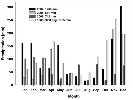
Petriccione et al. (Petriccione et al., 1993), it their study around the Amplero local scale, classified the climate of the site in the same way, as mountainous Mediterranean with no summer drought. Long-term mean annual precipitation is 1365 mm and annual mean temperature is 10°C (ARSSA local database).

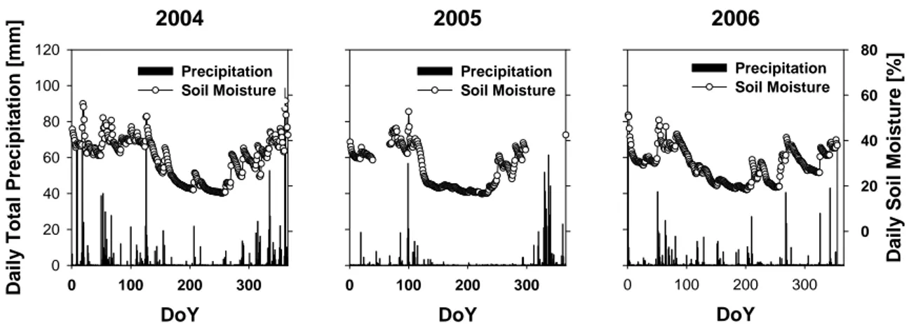
During the time period our field campaign were carried out (2004, 2005 and 2006) the mean annual temperature was 8.5, 8.6 and 9.6 °C respectively and total annual precipitation was 1269, 681 and 742 mm, respectively (Figure 4). In particular, in 2004 and August 2006 there was a mild summer drought, while between June and September 2005 precipitation was absent, leading to a strong dry period that limited carbon grassland uptake and pasture re-growth after the cutting. M o n th D ec-0 3 F eb -0 4 A p r-0 4 Ju n -0 4 A ug -0 4 O ct-0 4 D e c-0 4 Mon th ly air t e m p er at u re [° C] 0 1 0 2 0 3 0 4 0 5 0 To ta l mo n thly r a in [ m m ] 0 2 0 4 0 6 0 8 0 1 0 0 2 0 0 4 0 0 6 0 0 8 0 0 1 0 0 0 T em p e ra tu re R a in Am p le ro (8 8 4 m ) 9.4 6 12 6 9 .3 2 0 0 4 2 2 .4 1 5 .5 6 .9 -1 3 .4 M o n th D e c -0 4 F e b -0 5 A p r-0 5 J u n -0 5 A u g -0 5 O c t-0 5 D e c -0 5 M onthly air tempe ra ture [°C ] -1 0 0 1 0 2 0 3 0 4 0 5 0 Tota l monthly ra in [mm] 0 2 0 4 0 6 0 8 0 1 0 0 2 0 0 4 0 0 6 0 0 8 0 0 1 0 0 0 T e m p e ra tu re R a in A m p le ro (8 8 4 m ) 8 .5 7 6 8 1 .2 2 0 0 5 2 2 .2 1 6 .5 7 .3 -6 .5 M o n th D e c -0 5 F e b -0 6 A p r-0 6 J u n -0 6 A u g -0 6 O c t-0 6 D e c -0 6 M o n thl y ai r te m p e rat u re [ °C] 0 1 0 2 0 3 0 4 0 5 0 T o ta l mo nt hly rai n [ m m] 0 2 0 4 0 6 0 8 0 1 0 0 2 0 0 4 0 0 6 0 0 8 0 0 1 0 0 0 A m p le ro (8 8 4 m ) 9 .7 0 7 4 2 .2 2 0 0 6 2 4 .7 1 5 .9 4 .4 -8 .5 T e m p e ra tu re R a in

Figure 4 - Walter and Lieth diagram for 2004 (a), 2005 (b) and 2006 (c).

a)

b)

1.6.2 Grassland characteristics and management

Vegetation composition of the Amplero grassland was characterized during the field campaign in 2004. The study area is mainly composed of few dominant graminoids (Poa 15%), forbs (Trifolium 30%, Medicago 20%) and composites (Geranium 20%, Cerastium 20%).

The soil is poorly to a bit poorly drained, and it is defined as a Haplic Phaeozems (WRB, 2006). The humus type is Rhizomull (Green et al., 1993). Soil depth is more than 1 m, and drainage ranges from poorly to imperfectly. The percentage of clays is 56% and pH is 6.5. Roots reach down to 15 cm and 90% of roots is fine.

AMPLERO

AMPLERO

AMPLERO

Figure 5 - Corine Land Use map (level IV)

According to the Corine Land Use classification (level IV), Amplero land use is extensive cropland; this classification includes managed grassland as well (Figure 5). Starting from the last 50 years, after been cultivated for some years, the area has been managed by a combination of cutting/harvesting and cattle grazing. The grass is nowadays cutted during the last week of June and later used for the cows, horses and donkeys grazing till the end of the year. Since grazing in the Amplero site is free it is difficult to calculate its precise impact of the area. The

Chapter I - Introduction

estimated stoking rate is around 0.3 animals per hectare each year. Comparing this value to the potential stoking rate of this pasture, it makes sense to hypnotizes that the grazing is extensive and that its effects are negligible on carbon balance.

The Amplero site is equipped with an eddy covariance tower for continuous measurements of CO2 and H2O. On the tower there are also all meteorological sensors for climate monitoring of

the site. The entire/whole equipment (meteorological and eddy sensors) are briefly described in the material and method section (par. 2.7.2).

Chapter II

Materials and Methods

2.1 Set-up of the field work

The optimal use of radiometric measurements and of remote sensing imaging processing can be achieved through a complete and accurate set of field measurements support. For this reason, during the research study we planned to collect the following field data:

♣ Biometric sampling;

♣ Both periodic or in continuous radiometric measurements; ♣ Satellite image acquisitions;

♣ Meteorological and fluxes measurements.

During the field surveys, we analyzed three distinct grassland typologies present in the whole Amplero area (Figure 6):

♣ Meadow, managed by harvesting and grazing that is the typical management in Amplero;

♣ Natural, delimitated by fenced areas to exclude all external impacts (clipping/harvesting and grazing);

♣ Pasture, used for animal grazing.

Furthermore, all of our campaigns were conducted in order to evaluate the use of hyperspectral and multi-spectral sensors to retrieve biochemical and biophysical variables and fluxes. All field measurements were concentrated on two approaches: the first one, based on radiometric measurements performed to support the link between canopy reflectance and biometric parameters of the vegetation (biomass, live biomass, dead biomass, leaf area index), and the second one, performed by continuous measurements and images acquisition on vegetation to support grassland land use mapping and biometric and fluxes forecasting.

Chapter II – Materials and Methods • Eddy tower 41°54’14.56 N 13°36’18.38 E • Fenced areas •Pasture area • Meadow e area • Eddy tower 41°54’14.56 N 13°36’18.38 E • Fenced areas •Pasture area • Meadow e area Meadow

Fenced areas: natural grass

Meadow

Fenced areas: natural grass

Figure 6 – In the upper part there is the satellite image of the study area of Amplero. The blue circle indicates the position of eddy station; yellow and white dashed areas represent pasture and meadow sampling areas, respectively, and red squares are fenced areas or rather natural plots. In the lower part there is a view of the fences.

2.2 Biometric

measurements

In this study the aboveground biomass (AGBtotal) refers to all collected plant material, including

live biomass (AGBlive), dead standing biomass and litter. This latter two categories fall into a

unique group, representing the total dead material on the grass (AGBdead).

Operatively, the measure of the aboveground biomass of grass vegetation in the Amplero site was based on the measurements of phytomass increment during the growing season, obtained through field sampling in different small plots (Lauenroth et al., 1986, Sala et al., 1988). From 2004 to 2006,for each grassland typology (meadow, natural and pasture), 3 or 5 small squares of 0.30 m x 0.30 m were randomly collected at intervals of one month or less. The dry weight of the grassland biomass was determined by clipping the standing biomass at the ground level.

In order to determinate the total amount of dry matter per unit of area [g m-2 _{or t d.m. ha}-1_{], all}

clipped material (AGBtotal) was sorted into the live leaves (AGBlive) and standing dead matter

(AGBdead), dried at 105°C for 48-72 h, and finally weighted. Contemporaneously to biomass

sampling, the leaf area index (LAI) of live leaves part of herbaceous clipped plants was destructively estimated using leaf area meter scanner (Licor LAI-3000).

In 2004, the root biomass was sampled taking 10 cores of soil of 8.5 cm diameter, between 0-15 cm. Based on 2002-2003 results, that showed that 89% of the fine roots are located in the first 15 cm of the soil profile, samples between 15 and 30 cm had not been taken.

In order to define the carbon content of above and below ground biomass, the IPCC methodology using the default conversion factor of 0.45 (IPCC, 2003) was used, whilst the total carbon and nitrogen content of Amplero soil was carried out at the University of Florence-Italy by Dr. Chiti using a Perkin-Elmer C/H/N analyzer 2400 (Chiti et al., 2007).

2.3 Assessment of NPP

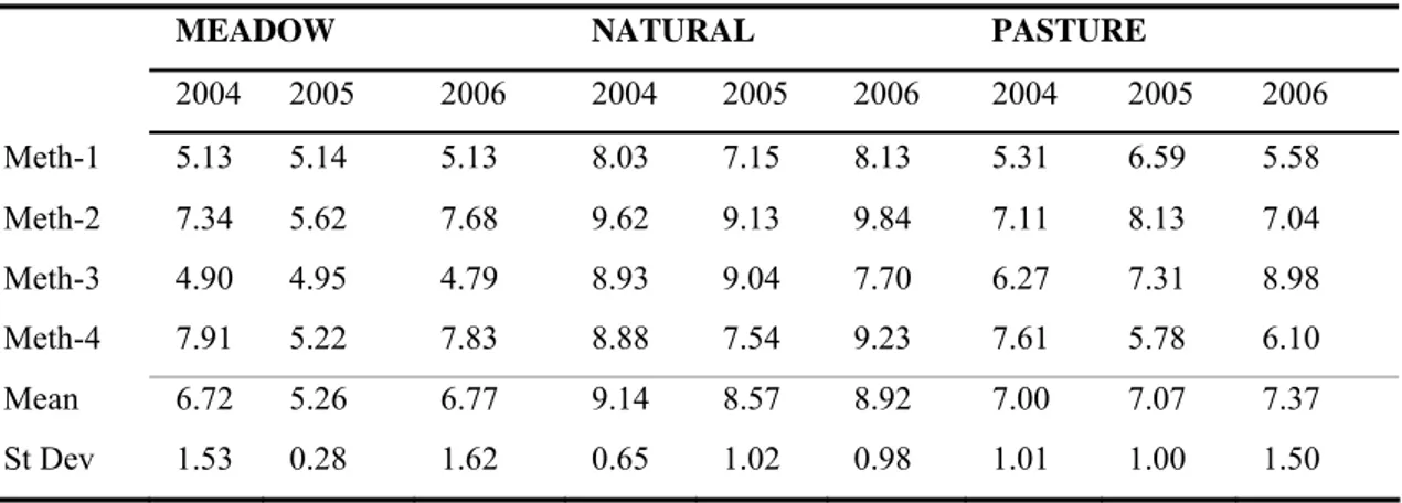
We utilized data acquired from biometric measurements conducted in 2004, 2005 and 2006 to compute the net primary productivity (NPP) of the three grassland managements.

According to literature information, six algorithms are often used to estimate NPP from biomass measurements in grassland vegetation: peak live biomass, peak standing crop (live plus standing dead matter), maximum minus minimum live biomass, sum of positive increments in live biomass, sum of positive increments in live and dead plus litter, and sum of changes in live and dead biomass with adjustment from decomposition (Long et al., 1992, Ni et al., 2004, Scurlock et al., 2002). However, each method differs in the number of inputs required to describe processes associated with biomass change over time (aboveground and belowground productivity, decomposition) and leads to different results in the assessment of NPP (Belelli Marchesini et al., 2007). Moreover, certain methods may be only applied within definite biomes (Scurlock et al., 2002).

Because of the high variability of inputs that each methods use to assess NPP, we chose to use two different approaches. First of all, we didn’t sampled below ground biomass (BGB) but we calculated NPP only from the field data of above ground biomass (Scurlock et al., 2002), modeling below ground biomass (BGB), and implementing the existent algorithm described by Gill et al. (Gill et al., 2002).

Among all methods reported by Scurlock (Scurlock et al., 2002), we selected the following four more adapted algorithms:

Chapter II – Materials and Methods

) ( AGBlive MAX

NPP =

Method 2 – Peak standing crop (Kucera et al., 1967, Long et al., 1989)

) (AGBtotal MAX

NPP =

Method 3 – Maximum minus (Long et al., 1989, Singh et al., 1975)

) (

)

(AGBlive MIN AGBlive

MAX

NPP = −

Method 4 – Sum of positive increments (Milner et al., 1968)

)

( AGBtotal

NPP

=

∑

∆

where AGBtotal is the whole aboveground clipped matter and AGBlive is aboveground live

biomass, both in g m-2 _{or t ha}-1_.

As highlighted above, and considering that the assessment of belowground productivity (BNPP: Below-ground Net Primary Productivity) is more difficult than the estimation of aboveground productivity (ANPP: Above-ground Net Primary Productivity) (Lauenroth et al., 1986), we predicted the BNPP of the Amplero site starting from the aboveground biomass (AGBtotal) that

can be roughly equivalent to ANPP and estimated from ANPP (Bradford et al., 2005). Moreover, we assumed that NPP derived from all four methods could be approximated to ANPP and thus included in the estimation of BNPP. In this way, we adjusted the algorithm proposed by Gill et al. (Gill et al., 2002) using the four different values of ANPP. We calculated BNPP using the following equation:

root T BGB liveBGB BGB BNPP ⎟∗ ⎠ ⎞ ⎜ ⎝ ⎛ = where:

BGB is the maximum yearly belowground biomass, in g m-2 or t ha-1;

BGB liveBGB

is the maximum proportion of BGB that is alive during the year and it is equal to 0.6 and Troot is the root turnover.

Doing the same assumption made from Gill et al. (Gill et al., 2002) and Bradford et al. (Bradford et al., 2005), we predicted the BGB:

(

10

)

1289

3

.

33

79

.

0

−

+

+

=

AGB

MAT

BGB

where AGBn is the value of above ground biomass obtained from each n measurement (n is

varied from 1 to 4 and refers to the number of applied methods) and MAT is the mean annual temperature, in K.

Finally, according to Gill and Jackson (Gill et al., 2000) we calculated root turnover from mean annual temperature:

MAT

root e

T =0.2884 0.046*

2.3.1 Statistical

analysis

Doing a Kolmogorov-Smirnov test we analyzed the distribution of data set of biomass and its components and consequently the applicability of the all statistic tests, such as the t-test and the ANOVA analysis.

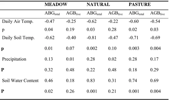
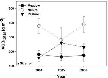
After that preliminary analysis by a paired t-test we investigated if the differences between the above ground biomass (AGBtotal, AGBlive and AGBdead) of the three grasslands typologies are

significant. In this manner we tried to evaluate the amplitude of the effect on biomass and productivity of the different management activity.

2.4 Hyperspectral proximal sensing: the FieldSpec PRO®

spectroradiometer

2.4.1 Radiometric

sampling

The solar radiation energy transits through the atmosphere to the vegetation canopy and it is again made available to the atmosphere by reflectance and transformation of radiant energy absorbed by plants and soil into fluxes of sensible and latent heat and thermal radiation through a complicated series of bio-physiological, chemical and physical processes (Huang et al., 2007).

Roughness, inhomogeneity and fragmentation of leaves influence the ideal reflection and define the scattering process of solar beams (Bolle et al., 2006). The bidirectional properties of leaves

Chapter II – Materials and Methods

have received little investigation contrary to plant canopies; for this reason most canopy reflectance models omit these characteristics of leaves and assume that leaves are Lambertian and scatter perfectly the solar light. The specular reflection on the leaf surface, however, affects the angular distribution of light and consequently the interpretation of remote sensing data. In some situations, like remote field experiments and laboratory measurements, the bidirectional reflectance, measured in terms of HDRF (Hemispherical Directional Reflectance Factor), can be recorded using a portable spectroradiometer and measuring leaf reflectance on both a black and a white background, alternately. The limit of this method is the strong dependency on the measurement conditions. According to Martonchik et al.(Martonchik et al., 2006):

)

,

(

)

,

(

)

,

(

_λ

_ϑ

_φ

φ

ϑ

λ

φ

ϑ

λ

,

,

=

,

L

L

HDRF

ϑr and φr are the angles of view (zenithal and azimuthally, respectively);

Lr is the radiance reflected by the target [W sr-1 m-2];

LrLamis the radiance reflected by an ideal Lambertian surface [W sr-1 m-2].

Practically, during field measurements, HDRF is estimated by measuring the total solar radiance incident on the target (Li) and dividing it by the reflected radiance upwelling from the target (Ls) in a given direction of observation (Meroni et al., 2006). Omitting the dependence of radiance from the angels of view and assuming incoming radiance into the target, as incoming radiance measured of the referent panel, reflectance (ρ) of target can be calculated as:

)

(

)

(

λ

λ

ρ

L

L

=

where Lt _{is the reemitted radiance by target and L}i _{is the incident solar radiance, both in watts}

per steradian per square meter [W sr-1 m-2].

2.4.2 Radiometric

characterization of the study area

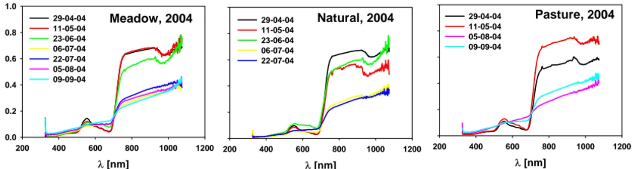
The vegetation of the three different type of grassland (meadow, pasture and natural, see Figure 6) was radiometrically characterized employing the HandHeld ASD spectroradiometer (ASD Inc, Boulder, CO, USA) (Figure 7). The spectral characterization of grasses was based on in

situ measurements; all spectra were collected during biometric measurements, just few minutes before the clipping and over the same square sampled plots.

The locations for the spectral characterization of the vegetation canopy were randomly sampled within the whole area of each of the three typologies. Depending on the stability of environmental condition during sunny days, five or ten spectral measurements per type of grasses were performed between 10:30 and 12:30 a.m., whereby each measurement was the average of 10 readings at the same spot. The sampling was carried out pointing at the centre of each square plot that was used in a latter stage for biomass clipping and partitioning. The spectral sampling was conducted by holding the ASD cosine optic in nadir position and supposing that the zenith and azimuth angular were approximated to zero; in addition, the distance above the ground was 150 cm, determining a field area of roughly 925 m2. As reported by Vescovo in his PhD study (Vescovo et al., 2005), this kind of optics seemed to give a better predictive power of vegetation biophysical characteristics that appeared to be related both to off-nadir direction of detected radiation and to the wider area which can be seen by the sensor. Even if weather conditions were constant, the spectroradiometer was calibrated regularly before each reading, using an integrated Spectralon® _{calibration panel and doing an up reading of the}

total incoming radiation in order to define the Lt _{of the equation for reflectance calculating.}

Table 2 - Technical characteristics of FieldSpec HH® spectroradiometer that was used during the field campaign.

FieldSpec® Hand Held Spectral Range 350-1050 nm

Spectral Resolution 1.4 nm @ 350-1050 nm Sampling Interval 0.7 spectra/second

Optics 25° (bare head), 1°, 10°, 20° and cosine Weight 5.7 kg or 12.55 lbs

2.4.3 Data processing of the grass spectra

Collected spectra values were first exported to ASCII files with the FieldSpec Pro® software. Single ASCII files were created for each separate spectrum. Subsequently, all data were imported into Matlab® for further processing as well as vegetation index calculation. Averages and standard deviations where computed for each reading of type of grassland and for each date, taking into account the separate measurements with a black and white background. A visual quality assessment was performed for every spectrum in order to identify incorrect

Chapter II – Materials and Methods

spectra with which they were removed. After the quality control, all data were imported into the Matlab® software to create three referential spectral libraries containing, per each typologies of management the all and the mean reflectance spectra and the white and black background.

Table 3 - Most used vegetation indexes

ID Algorithms Bibliography SR

SR

ρ

ρ

=

NDVI

ρ

ρ

ρ

ρ

+

−

=

Green

NDVI NDVIgreen

green nir green nir

ρ

ρ

ρ

ρ

ρ

ρ

ρ

ρ

ρ

ρ

(

(

₍

(

₎

)

)

)

₍

(

₎

)

WBI

ρ

ρ

=

Figure 7 – Handheld spectroradiometer FieldSpec PRO® (ASD, Bulder, Colorado)

Using statistical analysis we also tested at which bands the mean reflectance spectra of the three different grassland typologies were significant different. Our research hypothesis was tested using the one-way analysis of variance. The analysis of variance was used at different sampling

period such as week, month and year in order to evaluate the spectral differences for growing period of grasslands.

Considering that vegetation index calculation is a good method to remove the spectral variability due to the canopy geometry, the soil background, the sun view angles the and atmospheric conditions for estimating biophysical vegetation properties and fluxes as well as the biomass, Leaf Area Index (LAI), the percentage of green vegetation cover and the fraction of green vegetation (Baret et al., 1991, Becker et al., 1988, Gianelle et al., 2007, Gitelson et al., 2004, Gitelson et al., 2002, Huete et al., 1998, Pinty et al., 1992, Vescovo et al., 2006) most common vegetation indexes were automatically calculated in Matlab® _{environment. (Table 3).}

We analyzed the goodness of various vegetation index as predictors of biophysical parameters using the regression techniques (Gong et al., 2003). In general, for a bivariate regression model of a biophysical parameter (independent variable x) and a VI (dependent variable y), goodness-of-fit measures such as the coefficient of determination (R2_{), mean squared error (MSE), and}

root mean squared error (RMSE) are useful to indicate the vegetation index sensitivity to the biophysical parameter. (Ji et al., 2007). Moreover, the effectiveness of the regression was also evaluated using a covariance analysis.

2.5 MODerate-resolution Imaging Spectroradiometer

(MODIS)

The MODerate-resolution Imaging Spectroradiometer (MODIS), that was included in the EOS (Earth Observation System) project launched on 18 December 1999, is nowadays the keystone instrument on the Terra (EOS-AM 1) and on the Aqua (EOS-PM 1) missions, and it was sent into orbit in April 2002.

MODIS scanned the Earth’s surface every 1-2 days, making observations in 36 co-registered spectral bands at moderate resolution (0.25 - 1 km); of these bands, the first seven were used for the study of vegetation and Earth’s land cover. The first two bands (red at 620-670 nm and NIR at 841-876 nm) were acquired at 0.25 Km while the five following bands (blue: 459-479 nm; green: 545-565 nm; NIR: 1230-1250 nm and SWIR: 1628-1652 nm, 2105-2155 nm) at 0.5 km (Table 4). All MODIS products are free downloadable from its web site (http://modis.gsfc.nasa.gov).

Chapter II – Materials and Methods

Table 4 - MODIS band amplitude.

Reflected Solar Bands Emissive Bands

250 m 500 m 1 km 1 km B1: 620-670nm B3: 459-479 nm B8: 405-420 nm B20: 3.660-3.840 µm B2: 841-876nm B4: 545-565 nm B9: 438-448 nm B21: 3.929-3.989 µm B5: 1230-1250 nm B10: 483-493 nm B22: 3.939-3.989 µm B6: 1628-1652 nm B11: 526-536 nm B23: 4.020-4.080 µm B7: 2105-2155 nm B12: 546-556 nm B24: 4.433-4.498 µm B13L: 662-672 nm B25: 4.482-4.549 µm B13H: 662-672 nm B27: 6.535-6.895 µm B14L: 673-683 nm B28: 7.175-7.475 µm B14H: 673-683 nm B29: 8.400-8.700 µm B15: 743-753 nm B30: 9.580-9.880 µm B16: 862-877 nm B31: 10.780-11.280 µm B17: 890-920 nm B32: 11.770-12.270 µm B18: 931-941 nm B33: 13.185-13.485 µm B19: 915-965 nm B34: 13.485-13.785 µm B26: 1.360-1.390µm B35: 13.785-14.085 µm B36: 14.085-14.385 µm

2.5.1 MODIS data processing

To evaluate the comparability between values that were collected punctually at the field level by portable hyperspectral radiometer and the MODIS data acquired at satellite level with a broader wide bands and a bigger spatial resolution, spectra collected through the Field Spec Hand Held radiometer were firstly re-sampled at the different MODIS wide bands (See table above). Therefore, we directly acquired MODIS images at the same date of field surveys to scaling up the field relationship (Tab 5). We used NDVI and EVI products with a temporal resolution of 16 days and a spectral resolution of 250 m. Since images were acquired in a HDF-EOS format , they were opened and clipped using a MODIS tool provided directly from MODIS company. Images were already re-projected and atmospheric corrected.

The goodness of re-sampled MODIS vegetation indexes in predicting of grassland characteristic was tested by a the regression techniques and the covariance analysis.

The right position of the Amplero site was identified importing into images the coordinates (latitude and longitude) recorded through a portable GPS (Thales®, Mobile Mapper). To be

sure that extrapolated pixel corresponded to the Amplero grassland area, we considered the mean values of NDVI and EVI calculated from a square of 9 pixels centered on the Amplero site position. At this time all field data were averaged for/to a single sampling date/value to account the intrinsic pixel spatial variability due to the spatial resolution of the MODIS sensor.

Table 5 - Number of images and days of acquisition of the 16 days/EVI-MODIS and 16 days/NDVI-MODIS data. In order to interpolated biometric and sensed data we acquired the only images that corresponded to each date of the field surveys.

EVI-MODIS NDVI-MODIS N.of images Date N.of images Date 2004 7 113, 129, 161, 177, 193, 209, ₂₄₁ 7 113, 129, 161, 177, 193, _{209, 241} 2005 6 129, 145, 161, 177, 193, 225 6 129, 145, 161, 177, 193, ₂₂₅ 2006 3 113, 161, 145 3 113, 161, 145

2.6 Continuous NDVI measurements by CNR1 Net

Radiometer

In order to continuously collect NDVI of the grass of the Amplero site, in April 2005 we mounted the CNR1 spectroradiometer near to the eddy tower (Kipp & Zonen, Campbell In., Logan, UT) (Campbell et al., 2000). Considering that the field of view of CNR1 pointed directly to the meadow, we used these data only for studying the properties of the meadow, the more representative typology of grassland in Amplero site.

2.6.1 Partitioning of solar radiation into wavebands and estimation of

NDVIb

Data of solar radiation used for this part of work consisted in the measurements of the components (incoming and reflected) of the solar radiation and PAR (Photosynthetically Active Radiation) above the vegetation canopy at Amplero site.

The incoming and reflected PAR was measured by a two quantum sensor (SKP 215, Skye In., UK), while the components of solar radiation were measured continuously by the CNR-1 Net Radiometer (Kipp & Zonen, Campbell In., Logan, UT) with an average of 30-min. As shown in