particles in opposite sign dilepton
events with the CMS detector
Gigi Cappello
Facolt`a di Scienze Matematiche, Fisiche e Naturali
Universit`a degli studi di Catania
A thesis submitted for the degree of PhilosophiæDoctor (PhD) in Physics
Reviewer: Dr. Giuseppe Salvatore Pappalardo Ph.D. Coordinator : Prof. Francesco Riggi
Cover image:
di-muon event in CMS, sketch by Tom McCauley
Introduction 1
1 Theoretical overview 5
1.1 Beyond the standard model . . . 5
1.1.1 The Standard Model of elementary particles and in-teractions . . . 6
1.1.2 Limits of the Standard Model . . . 9
1.2 Supersymmetry . . . 15
1.2.1 Minimal Supersymmetric Standard Model . . . 16
1.2.2 Supersymmetry breaking and free parameters . . . . 21
2 The CMS detector at LHC 29 2.1 The Large Hadron Collider . . . 29
2.2 Compact Muon Solenoid . . . 33
2.2.1 Tracking system . . . 38
2.2.2 Calorimetry . . . 42
2.2.3 Muon detectors . . . 45
3 Supersymmetry at CMS 51
3.1 Physics at Hadron Colliders . . . 51
3.2 Monte Carlo simulation . . . 54
3.3 Supersymmetry searches at CMS . . . 56
3.3.1 Production . . . 56
3.3.2 Decay Chains . . . 58
3.4 SUSY studies . . . 59
3.4.1 mSUGRA Benchmark points . . . 59
3.4.2 cMSSM scans . . . 63
3.4.3 Simplified models . . . 64
3.5 Dilepton analyses . . . 67
3.5.1 Reference Analyses . . . 67
3.5.2 Opposite Sign dilepton events . . . 68
3.6 Main sources of background for OS dilepton analysis . . . . 69
4 Event selection, data and Monte Carlo simulation 75 4.1 Analysis objects . . . 75 4.1.1 Electrons . . . 76 4.1.2 Muons . . . 78 4.1.3 Isolation . . . 79 4.1.4 Jets . . . 84 4.1.5 MET and HT . . . 85 4.2 Pre-selection cuts . . . 86 4.3 Event selection . . . 89 4.4 Recorded datasets . . . 91 4.4.1 Trigger menus . . . 92
4.5 Monte Carlo validation . . . 93
4.7 Pile-up simulation . . . 95
4.7.1 Event reweight . . . 95
4.7.2 Jet and HT correction . . . 96
4.7.3 Correction of leptons isolation . . . 97
4.8 Systematics in Monte Carlo simulations . . . 99
4.9 Data/MC comparison . . . 105
5 ABCD estimate 113 5.1 Data-driven methods . . . 114
5.1.1 The ABCD method . . . 115
5.2 Discriminating variables . . . 117
5.2.1 In-analysis variables . . . 118
5.2.2 Out-of-the-analysis variables . . . 120
5.3 Setup of the method . . . 124
5.3.1 Definition of signal and control regions . . . 124
5.3.2 Correlation of the pairs . . . 134
5.3.3 ABCD estimate with Monte Carlo . . . 135
5.3.4 Separation of the signal . . . 140
5.3.5 Studies of robustness . . . 145
6 Discussion of results 153 6.1 Systematics of the ABCD method . . . 153
6.1.1 Toy Monte Carlo method . . . 154
6.1.2 Variation of the boundaries . . . 159
6.2 ABCD with √s=7 TeV data . . . 163
6.3 Exclusion limits . . . 166
6.3.1 Confidence level . . . 167
Conclusions 181 A Analysis software 185 B Data/MC comparisons 197 C ABCD pairs 215 References 225 List of Figures 235 List of Tables 249
The Standard Model of elementary particles and interactions (SM) is a suc-cessful theoretical apparatus, whose predictions have been experimentally proved with remarkable precision. Despite its impressive predictive power, the model has some theoretical and phenomenological limits, pointing to the existence of a more general theory, which the Standard Model can be thought of as a low-energy effective theory. The supersymmetric extension of the SM is among the most famous of these theories. Introducing a new symmetry to the model, known as supersymmetry, some theoretical issues (like the so called hierarchy problem) find an elegant solution. If super-symmetry exists (in the way it has been theorized), the supersymmetric partners of the SM particles should have masses not greater thanO(TeV). They could then be produced in p − p collision at Large Hadron Collider (LHC).
The LHC is a collider installed at CERN in the ∼ 27 km underground tunnel originally hosting the Large Electron-Positron collider (LEP). It started its operations in late 2009 with runs at center of mass energy of √s = 2.36 TeV. During the whole 2011 it operated at √s = 7 TeV delivering an integrated luminosity of ∼ 5f b−1. At the present (2012) p − p runs at√s = 8 TeV are ongoing.
Four big experiments are placed at four interaction points; two of them (ATLAS and CMS) are general purpose experiments, designed to accomplish many particle physics tasks, as the search for the Higgs boson and for supersymmetric particles.
In this thesis a search for supersymmetric particles in the data collected by CMS at√s = 7 TeV is presented. The search is focused on the selection of events characterized by:
• high missing transverse energy;
• high jet activity;
• two hard leptons of opposite charge.
This particular exclusive signature (which we refer to as opposite sign dilepton signature) has a very good background rejection power and should permit spectroscopic studies of the supersymmetric particles produced, once a sufficient amount of them is collected.
The bulk of the analysis consists on the isolation of the events of new physics, through the performance of some selection cuts on properly chosen discriminating variables. Even if, after this step, most part of the standard model background is actually rejected, an estimate of the background events still surviving (mainly top pairs production) is mandatory. The control of any residual background is made using data-driven techniques.
In this work, a particular data-driven method, involving many dis-criminating variables, is developed. An accurate setup of the method is absolutely necessary to obtain a correct data-driven estimate of the resid-ual background. This delicate step requires the usage of validated Monte Carlo simulations of the Standard Model processes.
The thesis is organized as follows:
In chapter 1 a brief theoretical introduction to supersymmetry is exposed. Some details of the supersymmetry breaking mechanism and of different models are given. The cMSSM (constrained Minimal Super-symmetric Standard Model) is introduced.
In chapter 2 the LHC and the CMS experiment are described. The main features and performances of the sub-detectors of CMS are illustrated.
In chapter 3 after a brief introduction about physics at hadron colliders and simulation of hard scattering processes, a description of su-persymmetric phenomenology at CMS is given. Different SUSY analyses are introduced; in particular, the opposite sign dilepton searches are de-scribed in more detail. Simplified Models (SMS) are also introduced as an alternative approach to the search with respect to the classical cMSSM scans.
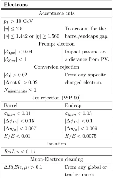
In chapter 4 the definition of the selection criteria of electrons, muons, jets, MET (missing transverse energy), and HT (scalar sum of jet’s transverse momenta) are exposed and the analysis cuts are discussed. The second part of the chapter is dedicated to the validation of Monte Carlo simulations of the Standard Model background. In particular, the effect of pile-up reweighting and of systematic uncertainties on MC are studied. In chapter 5 the Monte Carlo samples studied and validated in chapter 4 are used to develop and setup a data-driven method, called ABCD method.
In chapter 6 the ABCD method is applied on √s = 7 TeV data. The estimation obtained are used to set confidence limits in the cMSSM phase space.
Theoretical overview
A theoretical introduction to physics beyond the Standard Model is ex-posed. A brief analysis of the main issues related to the Standard Model permits to introduce a new space-time symmetry called Supersymmetry. Its main properties are discussed together with some details about its breaking mechanism.
1.1
Beyond the standard model
The Standard Model of elementary particles and interactions (SM) is a gauge theory based on the symmetry group SU (3)C ⊗ SU (2)L⊗ U (1)Y (color + weak isospin + weak hypercharge) spontaneously broken in SU (3)C⊗U (1)em(electroweak symmetry breaking) through a scalar Higgs filed. Although its extraordinary predictive power and phenomenologi-cal success, some theoretiphenomenologi-cal issues and open questions strongly point to ‘something else’: a more general theory, including new classes of parti-cles and interactions, of which the SM could be considered a low energy approximation.
lepton charge [e] quark charge[e] 1st family e -1 u +2/3 νe 0 d -1/3 2nd family µ -1 c +2/3 νµ 0 s -1/3 3rd family τ -1 t +2/3 ντ 0 b -1/3
Table 1.1: Fermions of the Standard Model.
Particle Field Group Mass [GeV]
gluons Gaµ SU(3)C 0
weak bosons W± SU(2)L⊗ U (1)Y 80.4 Z0 SU(2)L⊗ U (1)Y 91.2
photon γ U(1)em 0
Table 1.2: Bosons of the Standard Model.
1.1.1 The Standard Model of elementary particles and
in-teractions
Matter constituents and fundamental interactions are described as exci-tations of quantum fields. Matter fields are fermionic (spin=1/2), while gauge fields, related to the fundamental forces, have spin=1, i.e. they are bosonic[1]. Three of the four fundamental interactions are well described by the model while gravity is not included.
The basic bricks of the theory are quarks and leptons: the last ones interact only weakly and (if charged) electromagnetically , while quarks also strongly. Both species exhibit a three-family classification, whose origin still remains unknown.
(color-SU (3)) symmetry and is called quantum chromo dynamics (QCD). The carriers of the force (called gluons) are the eight generators of the symmetry group. Due to the non-abelian structure of the group, gluons interact not only with quarks but also with themselves (self interaction). This is the basis of distinctive features of the strong interactions, such as confinement and asymptotic freedom[2].
The complex phenomenology of weak interactions cannot be explained using a simple gauge group (as in QCD). Many experimental measure-ments show in fact a maximal C and P violation for weak interactions, suggesting that they can be described by a group for which left-handed fermions are doublets and right-handed ones are singlets (SU (2)-left). This however is strictly true only for charged currents (mediated by W± exchange) while neutral currents (mediated by Z0) also couple with right-handed particles, although with a different coupling constant (i.e. with a different strength).
This particular behavior is successfully considered in account within a theoretical framework first introduced by Glashow, Weinberg and Salam in which weak and electromagnetic interactions are unified under the sym-metry group SU (2)L⊗ U (1)Y. The hypercharge Y is different from the electromagnetic charge Q, although it is related to it by the GellMann -Nishijima formula[3]:
Q = I3+ 1
2Y (1.1)
where I3the third component of the weak isospin. The symmetry group of electromagnetic interactions U (1)em appears after the symmetry breaking of SU (2)L⊗ U (1)Y.
Since an explicit symmetry breaking would lead to non-renormalizable divergences, a spontaneous symmetry breaking mechanism (Higgs
mecha-nism) has to be introduced adding a new scalar isospin doublet Φ =φ + φ0 . (1.2)
The interaction with Φ provides masses to the W± and Z0 bosons (but clearly not to photons) and to the fermions.
Gauge-invariance is preserved even adding to the electroweak Lagrangian density a term:
Ls= (DµΦ)†DµΦ − µ2Φ†Φ − h(Φ†Φ)2 (1.3) with h > 0 and µ2 < 0, being Dµ the covariant derivative1 for SU (2)L⊗ U (1)Y. A negative µ2 < 0 guarantees an infinity of degenerate states of minimum energy, not SU (2)-invariant, whose vacuum expectation value is: ⟨0|Φ0|0⟩ = −µ2 2h ≡ v √ 2 (1.4)
After the spontaneous symmetry breaking the system is projected in a neutral vacuum state. The scalar particle associated to the Higgs field will then be a neutral boson of mass mH =−2µ2, called Higgs boson.
The masses of the fermions rise from Yukawa terms:
LY ukawa = f cfψ f Lψ f RΦ (1.5)
The mass of any single fermion mf will be proportional to v and to the Yukawa coupling cf.
1
Looking at the whole SM Lagrangian, we enumerate 18 free parame-ters:
• in gauge sector: 3 coupling constants (αs, g, g′);
• in Higgs sector: Higgs mass mH, Higgs parameter µ2;
• in Yukawa sector: 4 mixing parameters (θ1,2,3, δ13), 9 fermion masses mf.
1.1.2 Limits of the Standard Model
The first experimental evidences of the Standard Model were the dis-coveries of neutral currents (Gargamelle, 1973 [4]) and of W± and Z0 (UA1, UA2, 1983 [5]). During its data taking (1989 - 2000), the Large Electron-Positron collider (LEP) at CERN allowed extraordinary precise measurements of many SM parameters[6] (figure 1.1), all of them in perfect agreement with the theoretical predictions. Similar measurements have been performed by TeVatron at Fermilab[7] and Large Hadron Collider (LHC) at CERN. Recent efforts led the ATLAS and CMS collaborations at LHC to the discovery of a new boson with mass between 125GeV/c2 and 127GeV/c2 which seems to be consistent with a Higgs boson (figure 1.2) [8][9].
Despite these phenomenological successes, the SM suffers some formal inconsistencies and leaves many theoretical questions unanswered: the motivation of the three-families pattern, for example, or the origin of CP violation (which is closely linked to the matter-antimatter asymmetry) and hierarchy of neutrino masses do not find a solution within the SM. Will will however focus on other issues, more closely related to the intro-duction of supersymmetry.
Measurement Fit |Omeas−Ofit|/σmeas 0 1 2 3 0 1 2 3 ∆αhad(mZ) ∆α(5) 0.02750 ± 0.00033 0.02759 mZ[GeV] mZ[GeV] 91.1875 ± 0.0021 91.1874 ΓZ[GeV] ΓZ[GeV] 2.4952 ± 0.0023 2.4959 σhad[nb] σ0 41.540 ± 0.037 41.478 Rl Rl 20.767 ± 0.025 20.742 Afb A0,l 0.01714 ± 0.00095 0.01645 Al(Pτ) Al(Pτ) 0.1465 ± 0.0032 0.1481 Rb Rb 0.21629 ± 0.00066 0.21579 Rc Rc 0.1721 ± 0.0030 0.1723 Afb A0,b 0.0992 ± 0.0016 0.1038 Afb A0,c 0.0707 ± 0.0035 0.0742 Ab Ab 0.923 ± 0.020 0.935 Ac Ac 0.670 ± 0.027 0.668 Al(SLD) Al(SLD) 0.1513 ± 0.0021 0.1481 sin2θ eff sin2θlept(Q fb) 0.2324 ± 0.0012 0.2314 mW [GeV] mW [GeV] 80.385 ± 0.015 80.377 ΓW [GeV] ΓW [GeV] 2.085 ± 0.042 2.092 mt[GeV] mt[GeV] 173.20 ± 0.90 173.26 March 2012
Figure 1.1: Pull between fitted and measured values of some SM param-eters, performed by the LEP ElectroWeak Working Group (March 2012). From [6].
Figure 1.2: The CLsvalues for the SM Higgs boson hypothesis as a function
Gravity
Gravity is not included in the model. Looking at relative strengths of fundamental interactions it is clear that gravity is by far the most weak, so this lack in theory does not affects quantitative predictions at elec-troweak scale. Near the Plank scale (1019GeV) however this is no more true, so including gravity in a consistent theoretical framework becomes mandatory. Unfortunately this framework can not be the SM. Superstring theories are elegant solutions to this problem, but they uppermost require a supersymmetric extension of the SM.
Dark matter
Evidence of the existence of dark matter rose from pioneering observations of clusters of galaxies by Zwicky (Zwicky,1933[10]) and from the studies on rotation curves of spiral galaxies, both pointing to mass distributions dramatically different with respect to the ones obtained considering visible objects only (stars, dusts). More recent studies on cosmic microwave background anisotropies (WMAP, 2010[11]) confirm that only 4% of the energy density of the universe is condensed in baryionic matter, while another 23% is carried by dark matter. It has to be made of weakly interactive non-baryionc particles. Relativistic neutrinos (the so called hot dark matter candidates) can be ruled out, since they could not ever lead to the formation of galaxies and clusters. Numerical solutions of Bolzmann equations for relic density of dark matter[12] point moreover to masses in the range O(10GeV) < m < O(1000GeV). They shouldn’t be relativistic particles and are then called cold dark matter. The SM does not provide any good candidate for cold dark matter.
Unification of coupling constants
We can write down the Renormalization Group Equations (RGEs) for each of the free parameters of the SM, in particular for the three coupling constants[13]:
dai dt = bia
2
i (1.6)
where we used the notation
ai≡ αi 4π ≡ g2i 16π2, (gi = g ′ , g, gs) (1.7)
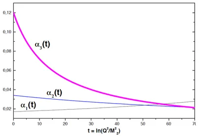
We should then study the evolution with scattering energy (Q2) starting from an initial value (µ2) as function of t = log(Q2/µ2).
Coefficients bi depend on the number of families of matter Nfam and of Higgs doublets NHiggsin the theory. Equations 1.6 admit the simple solu-tion
ai(t) = ai(0) 1 − bit
(1.8)
Considering, for the Standard Model, Nfam= 3 and NHiggs= 1, we imme-diately get each bi. As initial condition at t = 0 we can use the couplings at the Z-boson mass µ2 = MZ2, for which we have measurements from LEP[14].
α1(MZ) = 0.017 ± 0.001, α2(MZ) = 0.034 ± 0.001, α3(MZ) = 0.118 ± 0.003
Figure 1.3: Evolution of the gauge couplings in the Standard Model.
The evolution of the gauge couplings are shown in Figure 1.3. We first focus on the difference in behavior for α1 ∼ αQED and α3 = αs. The first function increases at large momenta, while the second one has very large values at small momenta and approaches zero at large momenta (small distances).
Another important thing we have to notice is a clear unification pattern shown by the evolution of the constants. The three gauge couplings seem in fact to unify at an energy of the order of 1015÷ 1016GeV, which can be seen as a hint of the existence of a great unified theory (GUT). In this scheme, MGU T ∼ 1016GeV should provide a natural and physically meaningful Λcutoff for renormalization scheme. However we have to warn about two issues:
• despite a qualitatively interesting unification pattern, the gauge cou-plings do not actually unify at exactly the same energy. The pa-rameters of the equations 1.6 should be tuned in order to give an
exact unification: this can be done only introducing other fields in the model, that is, admitting the existence of a physics beyond the Standard Model manifesting between MZ and MGU T;
• the unification scale pointed by the running couplings is very high compared to the electroweak symmetry breaking scale (∼ 102GeV). This creates a problem, called hierarchy problem, that will be now discussed.
Hierarchy problem
While the corrections to Higgs mass due to loops on SM fermions are maintained logarithmic by the chiral symmetry, the ones due to bosonic loops depend quadratically on the ultraviolet cutoff parameter. The one-loop corrected Higgs mass is than:
m2H(corr) ∼ m2H + cΛ2cutof f (1.9)
As just pointed, Λcutoff is of the same order of MGU T. This would drive the Higgs mass very far from the bare value. The theory is still renormal-izable, but the quantum corrections are several orders of magnitude larger than the the boson mass suggested by SM fits and measurements. This discrepancy is known as the hierarchy problem[15].
The only way to solve the problem without introducing any new physics beyond the SM is to imagine that every contribution to the correction at every loop level combines with the others in order to give acceptable mass values. Such a fine tuning however appears unnatural.
It should be noticed that bosonic and fermionic loops give rise to quadratic corrections whose c constants have opposite signs. We could
then imagine a fundamental boson-fermion symmetry, whose effect would be the cancellation of quadratic divergences at any level. If in fact there were equal numbers of fermions and bosons with the same couplings, equa-tion 1.9 would have the form:
δm2H ∼ −|c|(Λ2+ m2f) + |c|(Λ2+ m2b) = |c||m2b − m2f| (1.10)
Such correction has a value not larger than the Higgs bare mass (hence naturally small), if
|m2
b − m2f| < 1TeV2 (1.11)
This naturalness argument is of fundamental importance, since is the only hint that such a symmetry, called Supersymmetry, could manifest at TeV scale, then could be reachable by the Large Hadron Collider.
1.2
Supersymmetry
Supersymmetry is a space-time symmetry first introduced by Wess and Zumino in the early ’70s[16]. This symmetry transforms bosonic states into fermionic ones and vice-versa.
Q | B⟩ =| F⟩ (1.12)
Q†|F⟩ =| B⟩
The operatorQ transforms scalar wave functions into spinors, which means it behaves like an anti-commutative spinor[17]. The commutation rules for Q are:
{Q, Q†} = Pµ (1.14)
{Q, Q} = {Q†,Q†} = 0 (1.15)
[Pµ,Q] =Pµ,Q†= 0 (1.16)
being Pµ the generator of Poincar´e translations. From the last equation for µ = 0, we deduce:
Ef |F⟩ = P0(Q | B⟩) = QP0 |B⟩ = EbQ | B⟩ = Eb|F⟩ (1.17) then:
Ef = Eb (1.18)
i.e. supersymmetric partners must have the same mass if the symmetry is conserved.
1.2.1 Minimal Supersymmetric Standard Model
The Minimal Supersymmetric Standard Model (MSSM) is the supersym-metric extension which adds the minimum number of new fields to the Standard Model. The minimal hypothesis consists of giving a single super-partner to every standard model particle, that is, more formally, replacing
Superfield Fermions Bosons Particles Q (uL, dL) ( ˜uL, ˜dL) UC uR u˜∗R quarks/squarks DC dR d˜∗R L (νL, lL) ( ˜νL, ˜lL) leptons/sleptons EC lR ˜l∗R Φu ( ˜hu + , ˜hu 0 ) (φ+u, φ0u) higgsinos/higgs Φd ( ˜hd 0 , ˜hd − ) (φ0d, φ−d) Gi ˜g g gluinos/gluons Wi W˜ W winos/W’s B B˜ B bino/B
Table 1.3: List of the MSSM superfields.
every SM field with a single superfield. In particular we introduce a chiral supermultiplet for every fermionic and Higgs field in the Standard Model and a gauge supermultiplet for every gauge field in the Standard Model. The MSSM fields content is summarized in table 1.3.
The super-partners of fermions are spin=0 particles and are named by placing an s (from scalar) before the particle names (squarks, sleptons...). Bosons’ super-partners are spin=1/2 fermions named gauginos and hig-gsinos. The super-partner of the hypothetical graviton is called gravitino and has an important role in many supsersymmetric models.
While within the SM only one Higgs doublet is necessary to give mass to all particles, for the MSSM things are more complicated. It can be demonstrated[17] that two different doublets are necessary. This lead to 5 different Higgs bosons
The first two are neutral and scalar (in particular the lightest one, h, would be very similar to a SM higgs boson), A is a pseudo-scalar, and H± are charged and scalar.
The spontaneous electroweak symmetry breaking projects the two Higgs doublets in two different vacua (v and v) whose ratio
tan β = v
v (1.19)
is a free parameter whose role will be discussed later.
Mixing of the neutral gauge particles (wino, bino, neutral higgsinos) results in four mass eigenstates, called neutralinos ( ˜χ01 , ˜χ02 , ˜χ03 , ˜χ04) with the index increasing with mass. In the same way four charged gauginos, called charginos ( ˜χ±1 , ˜χ±2), are obtained through mixing of the charged winos and charged higgsinos. Similar mixing happens between left and right squark and slepton states, although these mixing are often negligible, except for the pair (˜tR , ˜tL), which mixes in (˜t1 , ˜t2).
We can write a supersymmetric Lagrangian density invariant under the standard model group[18]:
L = i (DµSi)†(DµSi) + i 2 i ψi ̸ Dψi+ + i 2 A λA̸ DλA− 1 4 A FµνAFµνA+ −√2 i,A g S† itAλA 1 − γ5 2 ψi+ h.c. + +1 2g A tA i S† iSi 2 +L(W) (1.20)
where ψi and Si are the spinor and scalar components of the superfield labeled by i, FµνA is the kinetic tensor for the gauge field A and λ a cor-responding quantity for the gaugino, while tA are the generetors of the symmetry related to the gauge field A. The first two rows in (1.20) are kinetic terms for every superfield, the third row and the first term of the last row are trilinear and quadratic couplings of fields. The last term L(W) depends on the so-called textitsuperpotential W. In the MSSM the superpotential has form:
W = µφuφd+ λuU QΦu+ λdD QΦd+ λeE LΦd (1.21) While this particular superpotential respects both lepton and baryon number conservation, the most general form of superpotential can also contain elements contributing to lepton and baryion number violating in-teractions. This terms however would have important phenomenological consequences, leading, for example, to a proton lifetime many order of magnitude shorter than the actual exclusion limits. In order to forbid such terms a new multiplicative quantum number, called R-parity is in-troduced, and its conservation is imposed. The R-parity is defined as
R = (−1)L+3B+2s (1.22)
with L and B the lepton and baryon number and s the spin of the particle. Clearly, according to this definition, SM particles have R = +1 while supersymmetric particles have R = −1. The conservation of R-parity has some important consequences:
• no mixing between SM and SUSY particles is permitted, which im-plies that baryon and lepton number violating interactions are for-bidden;
• in a collider experiment, SUSY particles can only be produced in pairs;
• once produced, a SUSY particle will decay into lighter particles fol-lowing a chain containing at least one SUSY particle per step;
• the lightest supersymmetric particle (LSP) must be stable.
LSP as cold dark matter candidate
The last item implies that the cosmological relic of LSP could be a good cold dark matter candidate. Since dark matter particles have to be only weakly interacting, good SUSY candidates are sneutrinos and lightest neu-tralinos ( ˜χ10). The firsts are ruled out by direct searches, so ˜χ10, which in-deed is the LSP in quite extended areas in the parameter spaces of many SUSY model, remains the only good candidate.
If the LSP is a neutralino, moreover, when produced in a collision experi-ment it could not be directly seen in detectors but, like a heavy neutrino, it should produce high amount of missing energy.
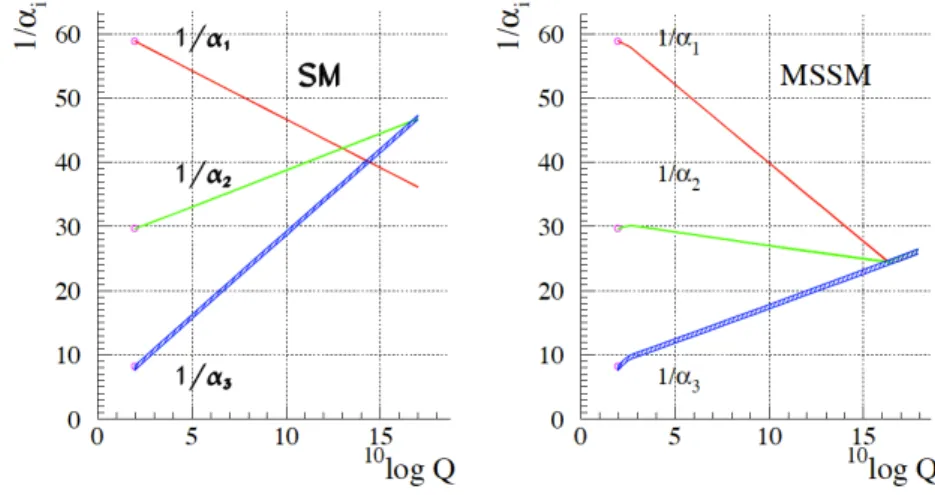
Evolution of gauge couplings in the MSSM
RGEs for gauge couplings have still form 1.6 with different biand NHiggs= 2. Evolution of the coupling constants are shown in figure 1.4. Since super-symmetric particles cannot contribute to the evolution of gauge couplings at low energies (under their masses), the curves will show a change in slope at energy MSUSY[19]
Figure 1.4: Evolution of the gauge couplings in the Standard Model.
MSUSY= 103.4±0.9±0.4GeV
Moreover, as we can see in figure, in a MSSM scheme the three gauge couplings actually unify at the same point
MGU T ∼ 1016GeV
that is compatible with many GUTs, like the Georgi-Glashow SU(5)[20]. It should be noticed that the unification of the three curves in a single point is absolutely not trivial because when introducing new particles all three curves are simultaneously influenced, leading to strong correlations between the slopes of the three lines. It can be shown, for example, that adding new generations or new Higgs doublets never yield unification[21].
1.2.2 Supersymmetry breaking and free parameters
Since the masses of the SM particles and their super-partners are not degenerate, equation 1.18 suggests that supersymmetry has to be a broken
symmetry. The solution of the hierarchy problem however points to mass differences not greater than the TeV scale. It is indeed the only theoretical limit we have about SUSY masses.
Up to now we do not know anything about the supersymmetry break-ing mechanism. We then use to parametrize our ignorance addbreak-ing an explicit soft breaking term to the MSSM Lagrangian
Lsoft= − i m2iS∗iSi− 1 2 j MjG˜jG˜j+ −auU ˜˜QH2− adD ˜˜QH1− aeE ˜˜LH1 (1.23) containing
• scalar mass terms (m2SS), in which m are 3x3 matrices; • gaugino mass terms;
• trilinear scalar interactions (aSSS), being a 3x3 coupling matrices. The full MSSM Lagrangian density contains then three terms:
LMSSM=Lgauge+LW+Lsoft (1.24) The first two terms do not introduce new free parameters with respect to the SM, since even SUSY particles interactions are ruled by the usual gauge couplings. The only new parameter is the additional VEV related to the second Higgs doublet (or, the more frequently used tan β). The soft term instead contains many new parameters (every M , m and a). Within the MSSM the total number of free parameters turns out to be 124[22]. It is a dramatically high number of degrees of freedom, since it introduce an unacceptable arbitrariness in the theory.
Constrained MSSM
A significant reduction of the number of free parameters can be performed introducing some constrains in the MSSM. A constrained MSSM (cMSSM) is a model in which is assumed that the symmetry breaking takes place in a ”hidden sector” having no direct relation to the MSSM sector. The breaking is mediated to the observable sector by a particular heavy me-diator X. The nature of the mediation is the distinctive feature of dif-ferent models. Between the most studied we enumerate gauge-mediated (GMSB), anomaly-mediated (AMSB)and gravity-mediated.
In the last case the gravity is the mediation interaction, so that MX = MPlank. The minimal of gravity-mediated models is called minimal super-gravity (mSUGRA).
In cMSSM, soft breaking parameters are assumed to be unified at GUT scales. In particular for mass terms and trilinear coupling:
M1= M2= M3 = m1/2 m2Q= m2U = m2D = m2E = m2L= m201 m2H1 = mH22 = m20 ai = A0yi
(1.25)
Thus there are only five free parameters left:
• m0: Universal scalar mass;
• m1/2: Universal gaugino mass;
• A0: Trilinear coupling at GUT scale;
Figure 1.5: RGEs solutions for scalar and gaugino masses in a mSUGRA scenario.
• signµ: Sign of the higgsino mass parameter.
Driving the RGEs for m and a down to the TeV scale (fig. 1.5) permits to build SUSY mass spectra as function of these five parameters[23]. In the mSUGRA scenario:
Charginos and neutralinos mχ˜0 2 ≈ mχ˜±1 ≈ mχ˜0 1 ≈ 0.8m1/2 (1.26) mχ˜0 3 ≈ mχ˜±2 ≈ mχ˜ 0 4 ≈O(|µ) (1.27) Gluino m˜g ≈ 2.4m1/2 (1.28) Sleptons m2˜l L ≈ m 2 0+ 0.54m1/2+ −1 2 + sin 2θ W m2Zcos 2β (1.29) m2ν˜ ≈ m20+ 0.54m1/2+ 1 2m 2 Zcos 2β (1.30) m˜2l R ≈ m 2 0+ 0.15m1/2− m2Zsin2θW cos 2β (1.31) Squarks m2u˜L ≈ m20+ (c + 0.5)m1/2+ 1 2− 2 3sin 2θ W m2Zcos 2β (1.32) m2d˜ L ≈ m 2 0+ (c + 0.5)m1/2+ −1 2 + 1 3sin 2θ W m2Zcos 2β (1.33) m2u˜R ≈ m20+ (c + 0.07)m1/2+ 2 3sin 2θ Wm2Zcos 2β (1.34) m2d˜ R ≈ m 2 0+ (c + 0.02)m1/2− 1 3sin 2θ Wm2Zcos 2β (1.35)
where 4.5 < c < 6.5.
The masses of gluino and lightest gauginos depend only on the universal gaugino mass m1/2, while the mass scale for scalar supersymmetric par-ticles are mainly ruled by m0. m1/2 also determines the mass splitting between right and left-handed scalars. These two parameters are then the most important in developing any search strategy and that is why exclu-sion limits are often shown in the m0 − m1/2 plane (also called cMSSM plane).
It has also to be noticed (from figure 1.5) that the parameter µ2+ m2 H2
runs to a negative value providing a natural way of generating a right shaped Higgs potential for the electroweak symmetry breaking.
Figure 1.6: h mass value in a mSUGRA scenario represented in the mSUGRA plane (left) and in the squark average - gluino mass plane. In these plots tan β = 30 and A0= −2m0 are imposed.
Notes on SUSY lightest Higgs boson
If the boson recently discovered at CERN is actually a Higgs boson, under the hypothesis of the existence of supersymmetry it would have to be the lightest supersymmetric scalar neutral boson h. Although it is absolutely premature, it is very interesting to notice that this discovery should lead to strong constrains on the cMSSM parameter space (Figure 1.6) and on the SUSY breaking model itself (Figure 1.7). In fact since many super-symmetric models require a light h (. 120GeV/c2), it seems that for this models the one just discovered should be a “border-line boson”. Some theoretical studies[24] show that a h boson with mass mh = 126GeV vir-tually rules out many constrained MSSM models, leaving mSUGRA as the most promising candidate.
O
VER
VIEW
Figure 1.7: The maximal h mass value, as function of tan β and of the universal scalar mass (here indicated with MS), for minimal Anomaly Mediated, Gauge Mediated, mSUGRA and some non minimal extensions.
The CMS detector at LHC
2.1
The Large Hadron Collider
The Large Hadron Collider (LHC)[25] is a two-ring collider installed at CERN (European Center for Nuclear Researches) in the ∼ 27km un-derground tunnel originally hosting the Large Electron-Positron collider (LEP) which operated there until 2000. The tunnel is situated under the French-Swiss border near the city of Geneva at a depth between 45m and 170m (figure 2.1).
The collider has been designed to provide p − p collisions at a center-of-mass energy√s = 14 TeV with a peak luminosity of L = 1034cm−2s−1, and P b − P b collisions at√s = 2.8 TeV/A.
The proton beams are pre-accelerated in the Proton Sincrotron (PS) and in the Super Proton Sincrotron (SPS) to an energy of 450 GeV and then injected to the LHC for the final acceleration, performed using RF electric fields of maximum frequency of 400 MHz. Beams are maintained in orbit by 1232 superconducting magnets providing a peak dipole field of 8.3T . The dipoles are operated at a temperature of 1.9K. At design
Figure 2.1: A scheme of LHC underground tunnel with interaction points and main experiments.
luminosity each beam will be made of 2835 bunches, of ∼ 1011 protons each, crossing every 25ns.
The luminosity delivered by a collider is based only on the beam pa-rameters. For gaussian-shaped bunches, it is given by:
L = kN
2f 4πσxσy
F (2.1)
where k is the number of colliding bunch pairs, N the number of pro-tons per bunch, f is the revolution frequency, σs are the beam sizes at interaction point and F is a factor related to the crossing angle. Lumi-nosity is a very important quantity since it is strongly related to the rate of a particular process:
Design July 2012
Beam Injection Energy (TeV) 0.45 0.45
Beam Energy (TeV) 7 4
Bunches per beam 2808 1374
Beam size (µm) 16 18
Protons per bunch 1.15×10¹¹ 1.5×10¹¹
Stored beam energy (MJ) 362 110
Table 2.1: LHC operation conditions.
R = L × σ. (2.2)
This means that having a high luminosity permits to investigate low cross sections processes. The luminosity integrated over the operation time (integrated luminosity, L) is usually measured as the inverse of a cross section.
LHC operation started in late 2009 with a pilot run at the injection beam energy of 450 GeV. In 2010 the center of mass energy was increased from 900 GeV to 2.36 TeV and then to half the design value, 7 TeV, reach-ing an integrated luminosity ofL ∼ 50pb−1 (Fig.2.2-a). During the whole 2011, LHC operated ad√s =7 TeV. TheL recorded by CMS experiment was 6.1 f b−1 (Fig.2.2-b). The 2012 p − p run is being performed at√s =8 TeV and will last till December. Up to August 2012 an integrated lumi-nosity L ∼ 7fb−1 has been delivered, that is expected to be about one third of the whole 2012 luminosity (Fig.2.2-c). After a technical stop in 2013, LHC will be driven at its design energy. A comparison between mid-2012 and design operation conditions is summarized in table 2.1[26]. Seven experiments are put along the tunnel at four interaction points
a)
b)
c)
Figure 2.2: LHC recorded luminosities in 2010 (a), 2011 (b) and first half of 2012 (c).
• ALICE (A Large Ion Collider Experiment): dedicated to studies of very high density strong interacting matter produced in heavy ion collisions[27];
• ATLAS (A Toroidal Lhc ApparatuS) and CMS (Compact Muon Solenoid): two general-purpose experiments with similar particle physics tasks, but adopting different experimental philosophies[28];
• LHCb: dedicated to studies of CP violating interaction in heavy quarks sector[29];
• LHCf (LHC-forward): two small electromagnetic calorimeters in the very forward regions of ATLAS interaction point, dedicated to π0 cross section measurements for cosmic rays physics[30];
• MoEDAL (Monopole and Exotic Detector At Lhc): specific pur-pose experiment for magnetic monopoles detection[31];
• TOTEM (TOTal Elastic and diffractive cross section Measurements): it shares the CMS interaction point. The detector is dedicated to measurement of total cross section and elastic scattering[32].
2.2
Compact Muon Solenoid
CMS (Compact Muon Solenoid ) is one of the four large experiments at LHC, dedicated, together with the ATLAS detector, to multi-purpose par-ticle physics measurements. It is located at Interaction Point 5, in France, 100 m below ground near the village of Cessy.
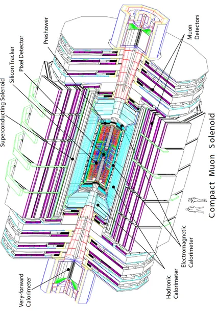
The detector (Figure 2.3) has a cylindrical shape with length of 21m and 15m of diameter. Its dimensions are more compact than the ATLAS ones but it is heavier (it weights approximately 12500t). The inner part of the
detector is put inside a solenoid producing a 4T magnetic field parallel to the beam lines. Outside the solenoid, the muon detectors are installed in the iron return joke frame. The experiment has almost a full solid angle coverage and it can be divided in three sectors: the central barrel and the two end-caps, installed at both sides of the barrel.
The design of the detector is motivated both by physics tasks and the specifications of the LHC. In order to accomplish the goals required by new physics, the experiment has been designed having:
• good inner tracking and pixel detection, with good τ and b-jet tag-ging;
• a very good, fast and redundant muon detector;
• high resolution and high granularity calorimeters;
• good missing transverse energy resolution.
Moreover, the challenging working conditions of the LHC make some char-acteristics mandatory:
• at design luminosity about 109 p − p collisions per second are ex-pected, thus a fast readout system and an efficient trigger are re-quired;
• high granularity and time resolution to handle with underlying events and pile-up;
• high resistance to radiation damage for sensors and readout elec-tronics.
The CMS sub-detectors are deeply described in ref. [33]. We now introduce just the main features of each sub-detector, from the interac-tion point to outer layers. We start with the tracking system (Pixel de-tector and Silicon Strip Tracker). We then describe the electromagnetic calorimeter (ECAL) and the hadronic calorimeter (HCAL). Outside the superconducting solenoid coil there is the muon system, made of Cathode Strip Chambers (CSC), Resistive Plate Chambers (RPC) and Drift Tubes (DT).
CMS conventions and important variables
A right-handed coordinate system is introduced with origin in the ge-ometrical center of the apparatus. The x-axis is oriented horizontally and points to LHC center. The y-axis is oriented vertically pointing upwards. The z-axis is then directed along the counterclockwise direc-tion of the LHC ring. With this frame definidirec-tion the azimuthal angle −π < φ ≤ π is determined in the x − y-plane while the polar angle 0 ≤ θ ≤ π is defined with respect to the positive z-axis. Once defined φ and θ we can build the transverse momentum and transverse energy:
pT = |p| sin θ ET = E sin θ
The missing transverse energy (MET) is defined starting from the measured energy of all visible particles:
MET = i Ei,x 2 + i Ei,y 2
A very useful variable in particle physics is the pseudo-rapidity η de-fined as η = −ln tanθ 2 .
A pseudo-solid angle ∆R is defined as a distance in the η − φ-plane:
∆R =
2.2.1 Tracking system
The innermost sub-detector is the tracking system. It consists of a pixel detector, whose main task is to define the position of the vertices, and a silicon strip tracker which performs precise measurements of momentum of charged particles, starting from their bending due to a homogeneous 3.8T magnetic field.
The system is totally based on solid state technology. It represents indeed one of the most massive ever usage of silicon detectors[34].
Near the interaction vertices a huge track multiplicity is recorded due to & 1000 minimum bias charged particles produced per crossing. High granularity, large hit redundancy and powerful track reconstruction algo-rithms are then necessary, together with materials resistant to high radi-ation doses.
The material budget moreover has to be as as thin as possible, in or-der to avoid photon conversions and bremsstrahlung that could affect the ECAL performances. The thickness encountered by the particle obviously depends on η, as shown in figure 2.4. This last requirement leads to con-strains on material budget and on the number of active layers.
The design adopted is shown in figure 2.5. The inner part is occupied by the pixel detector, while the Silicon Strip detector is divided in inner and outer regions along the radial coordinate and in barrel and end-caps (or disks) along η.
Pixel Detector
A vertex detector gives the position of primary and secondary vertices and the first seeds for track reconstruction. The technology adopted in CMS is that of pixels. Every pixel has a surface of 100 × 150µm2 and gives a
Figure 2.4: The tracker’s material thickness in radiation lengths as function of pseudo-rapidity. Contributions from active materials and other materials are shown.
digital signal related to the hit of a particle leaving an amount of energy over a threshold, fixed to a signal-to-noise ratio of 5. The total active area of 1m2 has in total 66 millions of pixels arranged in 1440 modules distributed over three barrel layers (|η| < 1.5) with radii 4cm, 7cm and 10cm and two disks per side at z = ±34.5cm and z = ±46.5cm. At least 3 hits are guaranteed for particles with |η| < 2.4.
Figure 2.6: A 3D view of the pixel detector.
The space resolution in the barrel region is 10µm along the r − φ-plane and 15µm along z. In the end-caps regions is 15µm along the r − φ-plane and 20µm along z.
Silicon Strip Detector
Outside the pixel detector a silicon strip detector covers a length of 5.6m and a radius between 0.2m and 1.2m, with a total surface of 225m2. The barrel region is equipped with ten layers of microstrips (four of them are
Resolution φ r(double-sided)
TIB 23-34µm 230µm
TOB 35-52µm 530µm
TID/TEC 15µm (low-r)
50µm (high-r)
Table 2.2: Resolution of the SSD.
double-sided), while every end-cap region (1.5 < |η| < 2.5) has three inner mini-disks and nine outer disks. The detector is divided in four parts:
• Tracker Inner Barrel (TIB), containing the four innermost layers of the barrel region. Strips are 300µm tick with a length of 7÷12.5cm and are parallel to the beam pipe;
• Tracker Outer Darrel (TOB), with the outer six barrel layers. Strips are ∼ 20 cm long and 500µm tick;
• Tracker Inner Disks (TID), containing the three mini-disks. Each disk has radial strips with thickness 300µm;
• Tracker End-Caps (TEC), with nine external disks, each divided in seven rings. The first three rings are equipped with 300µm tick strips while the last four has 500µm strips.
The space resolutions for each region are summarized in table 2.2. The two faces of the double-side detectors are mounted back-to-back at a stereo angle of 100mrad, providing a 3D view of the impact point.
The minimum number of hits for a almost straight track is always > 9. The tracking efficiency has been measured[35] to be > 98% for muons from
J/ψ decays. The transverse momentum resolution depends on pT and η. δpT pT = (1.5pT/GeV + 0.5)%, for |η| < 1.6 (3.0pT/GeV + 0.5)%, for |η| > 1.6 (2.3) 2.2.2 Calorimetry
A calorimeter gives a signal proportional to the energy released by a parti-cles passing through it. For a complete energy detection the particle must be completely stopped in the active material. The energy loss by photon or electrons involves other processes than that for hadrons. Thus different kind of detectors are necessary: electromagnetic calorimeters (ECAL) for photons or electrons showers, hadronic calorimeters (HCAL) for baryons and mesons.
Between the tracker and the coil in CMS an homogeneous ECAL is placed, followed by a sandwich HCAL.
Electromagnetic calorimeter
The CMS ECAL[36] is an homogeneous calorimeter made of 61200 lead tungstenate (PbWO4) crystals in the barrel and 7324 crystals in the end-caps. Each crystal has a projective geometry: in the barrel region, they are arranged in towers with internal surface of 22x22mm2, external surface of 26x26mm2 and depth of 230mm, corresponding to 25.8X
0 (radiation lengths). In the end-caps, towers are 28.6x28.6mm2 inside, 30x30mm2 outside and 220mm deep (24.7X0). Towers are moreover arranged in 5x5 clusters.
In the region between 1.65 < |η| < 2.6 a 20cm thick preshower detector is placed between the tracker and the end-caps’ ECAL. It is made of two lead radiators interleaved with two silicon strip detectors. The preshower
add some radiation length to the ECAL and enhances the γ − π0 discrim-ination.
Figure 2.7: A scheme of the ECAL.
The lead tungstenate has been chosen because of its fast scintillation response and of its hardness to radiation damage. It has moreover a small Moliere radius.
The energy resolution follows the function:
δE E 2 ≈ a √ E 2 + b E 2 + c2 (2.4)
where the energy is expressed in GeV. The first term is a Poisson term, with a = 2.8% (barrel), 5% (end-caps). The second is a noise contribution with b = 125 MeV (barrel), 500 MeV (end-caps). The constant term
c = 0.18 is obtained from early measurements[37], and is lower than the expected value of 0.3.
Hadronic calorimeter
Between the ECAL and the solenoid (at 1.77m < r < 2.95m), the CMS HCAL is a sandwich calorimeter with layers of copper radiators and plas-tic scintillators[38]. Copper is a high radiation length material without ferromagnetic properties (so suitable for working in a strong magnetic field). In the barrel region the HCAL is divided in 16(η)x18(φ) towers of thickness 5.4λ (absorption lengths). This depth is not sufficient to fully contain an hadronic shower, so two other layers are placed outside the coil at |η| < 1.26, the so called Outer Hadron Calorimeter (HO).
A similar pattern (without HO) can be observed in the end-caps (1.3 < |η| < 3). The granularity is ∆η × ∆φ = 0.087 × 0.087 for |η| < 1.6 and ∆η × ∆φ = 0.17 × 0.17 for |η| > 1.6. The total λ in this region is 10.
The energy resolution can be parametrized as:
δE E 2 = 85% E 2 + (7.4%)2 (2.5)
for energies between 30GeV and 1TeV.
At ±11.15 m from the interaction point the Hadron Forward Calorime-ter (HF) covers a pseudo-rapidity up to 5. It is made of steel absorbers and quartz fibers as active material. Such a robust design is mandatory since in the forward region the hadron rate is very high.
2.2.3 Muon detectors
The region outside the coil is completely dedicated to muon identifica-tion. Muons are the less stopped in material between all charged particles and are the only which can trespass the calorimeters. CMS has a very challenging and redundant muon system[39]. It consists of three different kind of detectors: drift tubes (DT), cathode strip chambers (CSC) and resistive plate chambers (RPC). They are arranged as shown in figure 2.8. The overall active surface is 25000m2.
Figure 2.8: A sketch of the muon system in CMS.
At |η| < 1.2 four layers of DT are alternated to the iron wheels of the return yoke. The muon system is then still inside a return magnetic field of ∼ 2T, oriented backwards with respect to the inner field. Muons in this region are bended in the reverse direction drawing a characteristic S-shaped trajectory. The space resolution in the central region is ∼ 100µm. In the end-caps (0.9 < |η| < 2.4) CSCs are mainly used because of
their better performances in higher multiplicity environments. As in the central region, we count four layers of chambers perpendicular to the beam line. The space resolution is ∼ 200µm.
RPCs are used both in the barrel and in the end-caps. Their very fast response (time resolution is 3ns) makes them a perfect trigger system for the CSCs and DTs.
A combined determination of the muon momentum using the tracker and the muon system leads to a very good resolution:
δpT pT
= apT/TeV (2.6)
with a depending on pseudo-rapidity. In the barrel, for pT = 1 TeV a resolution of 4% is obtained, degrading to 10% in the end-caps. For pT = 10GeV, the central resolution is 0.5%. First data from cosmic rays and from collisions confirm that the muon system is working at design resolution[40][41].
2.2.4 Trigger and Computing
At design luminosity (1034cm−2s−1) about 109 collisions per second are expected, corresponding to a data-stream of ∼ 100TByte/s. By now, a computing system capable to manage such amount of data does not exist. Moreover not every event contains interesting information from a physical point of view, so the main task of the trigger system is to perform a rapid event selection reducing the event rate to 100Hz (a reduction of a factor 106). The CMS trigger consists of two steps: a hardware trigger (Level 1 - L1) and a software based high level trigger (HLT)[42].
Level 1 trigger
A first fast selection is preformed via hardware, analyzing only few topical information from muon system and calorimeters with reduced granularity. As result of this raw but very fast analysis some so called primitives (for example muons or calorimetry deposit over a threshold) are required for a positive trigger response. The level 1 trigger conditions are common to almost every analysis, so having a static hardware trigger does not rep-resent an unacceptable limit. On the other hand the gain in speed with respect to a more ductile software system is huge.
The trigger is made of a chain of electronic steps, each performing a par-ticular selection with rates compatible with the bunch-crossing time. The whole maximum decision time is 3.2µs and is limited by the maximum latency time of data in the pipeline memories integrated in the front-end electronics. The L1 output rate is limited to 30kHz, leaving a safety mar-gin from the 100kHz design value.
High level trigger
At such a lower rate, a flexible software trigger can be used. The high level trigger runs on a filter farm with over 1000 CPUs each processing a single event. At this level the trigger uses information from all the sub-detectors at full resolution (the full event information is built after L1 decision by a builder network with a maximum data flow of 100 GBytes/s). A HLT decision takes less then 40ms and the final event rate is 100Hz, which is sufficiently small to be recorded for the off-line analysis[43].
Computing
In CMS ∼ 1PByte of data is produced every year. The HLT output events are reconstructed at a CERN facility called Tier0. Data are then distributed to several computing servers all over the world (Tiers1 and Tiers2 ) for direct access. Every tier is connected to each other through the computing Grid. The access to any data in the grid can be done using the CRAB tool[44].
Supersymmetry at CMS
As discussed in Chapter 1, the hierarchy problem points to the existence of some new physics beyond the Standard Model at TeV scale, i.e. at energies reachable by the LHC. Moreover, at design luminosity, the production rate for supersymmetric particles could be high enough to permit a discovery1.
In this chapter a description of supersymmetry phenomenology at CMS is exposed, after a brief introduction about physics at hadron colliders and simulation of hard scattering processes. Different SUSY analyses are introduced together with their discovery power. A particular attention is dedicated to the opposite sign lepton searches, which are the main subject of this thesis.
3.1
Physics at Hadron Colliders
Hadron collisions are much more complex than electron ones, since protons are not elementary objects. A proton is made of gluons, valence quarks
1For example, assuming an inclusive cross section ofO(1)fb for a SUSY process, we
and sea quarks, each one carrying a fraction x of proton’s momentum. Given an energy scale Q2 the probability for a certain constituent i of carrying a momentum fraction x is given by a parton density function (PDF) fiP(x, Q2).
Proton PDFs can be obtained from experiments at other colliders, like HERA[45], and extrapolated to LHC energies[46] (Figure 3.1 a) and b)).
a)
b)
Figure 3.1: a) Gluon and parton PDFs measured by HERA at Q2 =
10GeV2. b) Scatter plot x vs. Q2for production of an object of mass M and
rapidity y at LHC design energy. Current experimental constrains are also shown.
Gluon and parton PDFs have to be taken into account when calculating the cross section of a hard process. We consider for example the squark-gluino production:
Hadronization
Decay chain
Figure 3.2: Full p − p scattering including the hard SUSY process q + g → ˜
q + ˜g.
q + g → ˜q + ˜g (3.1)
Its cross section in a collision between proton A and proton B at a certain Q2 can be expressed as function of PDFs fP
i (x, Q2) and of the cross section of the elementary process (dˆσ(q+g→˜q+˜g)):
dσ(A+B→˜q+˜g+X)= q,g 1 0 dxq 1 0 dxgfiP(xq, Q2)fiP(xg, Q2)dˆσ(q+g→˜q+˜g) (3.2)
In figure 3.2 a typical p − p process is schematized, including the hard scattering 3.1, that is the circled part. All the other processes occurring are called underlying event and their knowledge is fundamental to correctly understand and simulate the detector’s response.
The underlying event consists of
• Initial and Final State Radiation (ISR/FSR), also called parton showering. It is the radiation of gluons or quark pairs from any colored particle involved in the event. It is often studied developing perturbative QCD calculations.
• Beam remnants: partons that do not take part to the hard pro-cess produce color singlets giving an important contribution to the particle flux especially in the high-η/low-pT regions.
• Hadronization. Every colored particle produced in decay chains, in ISR/FSR, or in beam remnants will arrange with others, pro-ducing hadrons. The study of hadronization processes requires non-perturbative QCD models.
3.2
Monte Carlo simulation
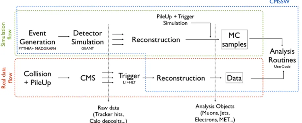
A full simulation of hard collisions consists of three steps: event genera-tion, simulation of detectors and event reconstruction. The whole simu-lation chain together with reconstruction of events in CMS is performed within a framework called CMSSW (CMS-SoftWare)[47], containing sev-eral thousands of packages, including generators, a GEANT4 simulation of the experiment[48], and several analysis kits.
Event generation
At generation level, hard scattering process, parton showering and hadroniza-tion are simulated. In CMSSW two different generators are used: PYTHIA6 [49] and MADGRAPH[50].
PYTHIA6 calculates the hard scattering process without additional par-tons. Radiated gluons or quark pairs are modeled as soft parpar-tons. This produces, under certain condition, simulated sub-leading jets softer than actually observed. Event generators like MADGRAPH solve this problem using a different approach called matrix element calculation, including ra-diated partons (up to 9) to the hard process simulation.
Hadronization is simulated in PYTHIA6 only, using a phenomenologi-cal model phenomenologi-called string fragmentation, where interactions between partons are modeled by colored string, whose breaking lead to the formation of hadrons.
Detector simulation
A detailed model of the CMS experiment (geometry and materials) is implemented in GEANT4. First of all every possible interaction of visible particles in a particular event is simulated, and the hits at sub-detectors are reproduced. In the second step, called digitalisation, the read-out electronic response to the hits is simulated. The final output has then the same form of any actual CMS data event and can be analyzed with the same tools.
For a complete simulation, two other effects have to be included: the trigger effect and the pile up interactions. They will be discussed in detail in the next chapter.
Figure 3.3: Simulation and data flow. The steps managed by CMSSW are underlined in blue.
3.3
Supersymmetry searches at CMS
3.3.1 Production
In a p − p collision at LHC, squark, gluinos, neutralinos and charginos can be directly produced. Under the hypothesis of R-parity conservation these particles would be produced in pairs. Since strong production are favored with respect to electroweak productions, if they are kinematically permit-ted, we mainly expect production of squarks and gluinos pairs. Three cases are possible (Figure 3.4):
• m˜g ≫ mq˜. The production of two squarks is dominant;
• m˜g ≪ mq˜. The production of two gluinos is dominant;
• m˜g ∼ mq˜. Diagrams involving the production of squark pairs, gluino pairs and squark-gluino pairs give similar contributions.
Figure 3.4: Diagrams of the production of squark and gluino pairs.
Figure 3.5: cMSSM plane with contour lines defining regions in which squarks are lighter than gluino, squarks are heavier than gluino, and mg˜∼
These possibilities define different regions in the cMSSM plane, as shown in figure 3.5.
If squark and gluinos are too heavy to be produced at LHC (Figure 3.6), electroweak production of neutralinos and charginos become impor-tant. The study of these processes is more complicated since neautrali-nos and chargineautrali-nos are mixed states of gaugineautrali-nos and higgsineautrali-nos. In a scan the cMSSM space then, even the matrix elements change, modifying the weights of different diagrams.
Figure 3.6: Production cross section for SUSY particles as function of the gluino mass. Are analyzed the conditions tan β = 3, signµ = +, and degeneration of squark masses. In the left side mg˜= mq˜is supposed, while
the in the right plot m˜q= 2m˜g is considered.
3.3.2 Decay Chains
Under R-parity conservation, once produced, squarks and gluinos decay following chains with a SUSY particle at every step and ending with the LSP ( ˜χ01 in the most area of cMSSM plane).
If squarks and gluinos are between the lightest SUSY particles, these chains are quite short. If instead they are heavier, cascades are
topo-logically more complex (figure 3.7). However, a generic SUSY signature involves:
• high jet multiplicity, especially in long chains, with high pT, due to the high mass of the parent particle. This leads to high scalar sum of the transverse momentum of the jets (high HT signature);
• large missing transverse energy, related to the escape of ˜χ01 (high MET signature);
• possibly, one or more hard leptons can be produced during the cas-cade (leptonic signature).
The last item is very important for our analysis and will be discussed in more detail in the next sections of this chapter.
A typical decay chain, involving all the signatures presented is shown in figure 3.8.
3.4
SUSY studies
3.4.1 mSUGRA Benchmark points
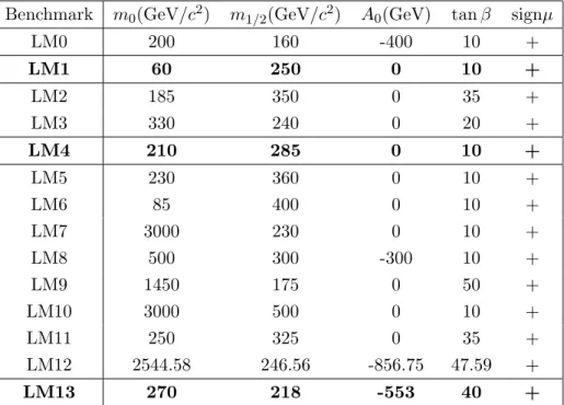
In order to develop search strategies covering different phenomenological scenarios, some benchmark points (i.e. some particular points in mSUGRA parameters space) have been chosen by the CMS collaboration. Focusing on one point (or on a small set of points), Monte Carlo analyses based on a detailed and precise detector simulation (fullsim) ca be performed. We count 14 low mass points (LM0-LM13), characterized by relatively low mass spectra (then suitable for an early discovery), and 4 high mass points (HM1-HM4). The parameters of the LM points are defined in table 3.1 and their position in the cMSSM plane is shown in figure 3.5.
Figure 3.7: Possible decay modes and branching ratios of a gluino in a high-mass test point of mSUGRA parameters space.
Figure 3.8: Feynman diagram of a chain starting from a squark, leading to the production of jets, leptons and high MET.
Benchmark m0(GeV/c2) m1/2(GeV/c2) A0(GeV) tan β signµ LM0 200 160 -400 10 + LM1 60 250 0 10 + LM2 185 350 0 35 + LM3 330 240 0 20 + LM4 210 285 0 10 + LM5 230 360 0 10 + LM6 85 400 0 10 + LM7 3000 230 0 10 + LM8 500 300 -300 10 + LM9 1450 175 0 50 + LM10 3000 500 0 10 + LM11 250 325 0 35 + LM12 2544.58 246.56 -856.75 47.59 + LM13 270 218 -553 40 +
Table 3.1: mSUGRA low mass benchmark points. In bold: the three points analyzed in this work.
Although these points cover a wide range of different mass spectra (and then production and decay scenarios), they are all characterized by having ˜χ01 as LSP and being compatible with cosmological measurements performed by WMAP, thus they all admit a SUSY particle as Cold Dark Matter candidate.
The three points underlined in table 3.1 (LM1, LM4, LM13) have been studied in this work. Given the benchmark point particle masses are cal-culated by a routine called SOFTSUSY[51]. In figure 3.9 the mass spectra for each point are shown. LM1 and LM4 are characterized by gluinos heav-ier than squarks, thus squark pair production is favored in these cases. In LM13 squark and gluino masses are similar so both productions occur with the same probability.
A particular feature of LM1 is that sleptons have masses intermediate be-tween those of the two lightest neutralino. This makes possible a particular sequence of two-body decays:
˜
χ02 → l + ˜l → l++ l−+ ˜χ01
leading to an opposite sign lepton pair whose invariant mass shows a characteristic end-point (Figure 3.8).
Is important to notice that two of these points (LM1, and LM4) have been already excluded by direct searches in CMS 1. This fact however has no importance for our work, since we do not aim to prove if SUSY exists at one of these benchmark points. They are actually used only as a set of different phenomenological possibilities on which our methods can be tested.
1
LM1
LM4
LM13
Figure 3.9: mSUGRA mass spectra for three benchmark points (LM1, LM4, LM13).
3.4.2 cMSSM scans
A scan of a large part of cMSSM plane is of fundamental importance in computing exclusion limits or evaluating the discovery potential of a certain analysis. It however requires the production of a very large
num-ber of samples. They cannot be produced with a full detector simulation (which takes on average some minutes per event for a complete simu-lation and reconstruction). For this purpose, a faster but less detailed simulation, called fastsim, can be made[56]. A fastsim, uses a simplified geometry model and some parametrization obtained from fullsims. The output samples are similar to those obtained with fullsim, hence the same analysis tools can be used. A typical SUSY event requires ∼ 1 second to be completely fast-simulated.
3.4.3 Simplified models
SUSY searches have been historically focused on particular constrained models. cMSSM however covers only a limited set of possible mass spec-tra and mass splitting, due to the strong relations between masses within these models. Moreover many production and decay channels contribute to each benchmark point in a strongly model-dependent way. There are two possible ways to go beyond the cMSSM. The first is to consider a more generalized model (e.g. pMSSM[57]), the second is to describe dis-covery potentials and exclusion limits in term of simplified models. The interpretation of CMS results using these more flexible models is an use-ful alternative and complementary approach to the traditional cMSSM analyses.
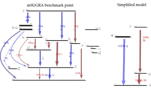
In a simplified model a limited set of hypothetical particles and decay chains is considered, matching to the experimental results of a specific search channel. The free parameters of these models are then the particle masses and the branching ratios. Each simplified model spectrum (SMS) consists of a small list of new hypothetical particles involving one or few more topologies. They can be seen as blocks of more complete models
Figure 3.10: (Left) Mass spectrum and branching ratios for a specific mSUGRA benchmark point. (Right) The SMS starting from the same par-ticles and involving the production of the same intermediate gaugino.
(Figure 3.10). Every topology has a codename which summarizes infor-mation about parent particles, chain length and, optionally, final states. For example, the topology:
T1bbbb
is characterized by the production of gluino pairs, directly decaying to LSP with two b-jets per leg in the final state (Figure 3.11).
In general, the first letter is always a “T” (for topology), followed by:
• 1,3,5 (odd numbers) when gluino-gluino are produced;
• 2,4,6 (even numbers) when squark pairs are produced;
Figure 3.11: Diagrams of a T1 simplified topology. In the right side the final states are specified (topology T1bbbb).
Other productions are not considered. Defined a production, the num-bers also specify intermediate states:
• 1,2: direct decay to LSP;
• 3,4: intermediate neutralino or chargino on one leg;
• 5,6: intermediate neutralino or chargino on both legs.
The CMS simplified models were chosen to cover a large part of the kinematic phase space of all considered final states. Limits are presented exclusively for each topology and the results are shown as a function of the masses of the particles involved (figure 3.12).
3.5
Dilepton analyses
3.5.1 Reference Analyses
Many different analysis strategies have been developed by the CMS SUSY group. Some of them look at events with jets and MET (hadronic searches), other make the more exclusive requirement of one or more leptons in the final state (leptonic searches). Depending on the final states involved, analyses are divided into groups called Reference Analyses (RA), orga-nized as follows
Hadronic Working group: • RA1 - Inclusive jet searches;
• RA2 - Exclusive jet searches (as subgroups: RA2b, RA2τ );
• Razor - This Analysis works with both hadronic and leptonic final states and is based on the construction of a dimensionless variable called razor (R)[59].