Modelling polymer-induced adhesion between charged membranes: theoretical and computational approach

MODELLING POLYMER-INDUCED ADHESION

BETWEEN

CHARGED MEMBRANES:

THEORETICAL AND COMPUTATIONAL APPROACH

A Thesis Presented to The Academic Faculty

by

Pannuzzo Martina

In Partial Fulfillment Of the Requirements for the Degree Doctor of Philosophy in Chemical Science

University of Catania

December 2011

INTRODUCTION 1

1. NUCLEATION THEORY WITH DELAYED INTERACTIONS 3

1.1. Schematic picture of the system 4

1.2. Formation energy of an adhesion patch 6

1.2.1. Bending Energy 6

1.2.2. Interaction energy 7

1.2.3. Bridging energy 8

1.3. Nucleation rate 9

1.4. Results and discussion 11

2. THERMODYNAMICS OF THE PSEUDO-TERNARY SYSTEM

POLYMER+IONS+ SOLVENT 14

3. POLYMER EFFECT ON THE ADHESION/FUSION RATE 20

3.1 Art state on PEG-mediated fusion: 20

3.2. Establishing new aspects of peg-mediated fusion 21

3.2.1. Approximate limiting cases 26

3.2.2. Self-regulating surface charges 27

3.2.3. Interaction between two charged surface in mixed

electrolyte-polymer-solvent fluid. 30

4. COMPUTATIONAL APPROACH 33

4.1 Coarse-Grained approach 33

4.1.1 Martini philosophy 34

4.1.2. The Model 35

4.2. Objective 36

4.3. Computational details 36

5. RESULTS AND DISCUSSION 40

5.2. Two charged membranes interacting with a pseudo-ternary system

polymer+ ions+ solvent 42

6. CATCHING THE FUSION EVENT 55

6.1 System evolution 55

6.1.1 Contact 55

6.1.2. Merging 58

7. Resume and CONCLUSION 62

ACKNOWLEDGEMENT 64

APPENDIX A 65

APPENDIX B 66

1

INTRODUCTION

Membrane fusion and fission are ubiquitous and fundamental processes in biological systems. Cells use them to transport material both between intracellular compartments and out of cells: this is the typical mechanism, e.g. for hormone secretion and for vesicle mediated synaptic transmission1,2,3,4.

Several chemical substances have an influence on the fusion rate. Most of them form tight ligand-receptor pairs between nearby membranes bringing them to contact distance from different membrane-anchored proteins1,2,3,4_{to simple divalent cations}4.

The addition of water soluble polymers that do not appreciably interact with the vesicles’ surfaces can dramatically enhance the adhesion/fusion rate5. The most common one is polyethylene glycol (PEG). If these same polymers are grafted to a vesicle’s surface they have, counterintuitively, the opposite effect6_{. The role of polymer-soluble}

polymers in triggering adhesion/fusion process between cells or vesicles has been explained in terms of osmotic forces related to the depletion of bulky polymer coils from the inter-membrane gap6. It is also well known that PEG condenses even charged macromolecules such as DNA7,8 _{, proteins}9_{, fibrils}10 _{and microtubules}11_.

The above scenario still remains complex even if we consider the mixing properties among ions, polymer and water alone, leaving aside their interactions with suspended particles like vesicles. The good solubility of ions in polymeric solutions or pure polymer melts is well documented due to its many technological applications12. However, it is also well-known that in polar solvents, such as water, ions might prefer the more polar aqueous environment. Studies of polymer-ion interactions in solvents of different polarity have been performed by several authors13,14.

When the solvation energy overcomes the polymer-solvent mixing entropy, ions induce a phase separation of the homogeneous solution leading to a polymer-rich phase coexisting with a polymer-poor solution in which most of the ions are dissolved. Such aqueous biphasic systems have been widely investigated due to their applicability as solvents in separation processes (for a recent review see, e.g., refs. 15 and 16) and proteins crystallisation17,18_.

2 depletion forces and polymers’ tendency to phase separate. The goal is to develop a self-consistent picture in which depletion, electrostatics and solvation forces are taken into account to determine the overall behaviour of membrane-membrane interactions in mixed solvents.

We do not explicitly investigate the outstanding polymer effect on the membrane fusion rate, rather we focus on the preliminary polymer-induced adhesion process which appears to be the clue for the following merging of the membrane leaflets. The rest of the thesis is organized as follows. In chapter 1 we discuss a semi quantitative theory to describe the adhesion kinetics between soft object via the nucleation and lateral growth of a localized adhesion site. In chapter 2, we develop a mean-field model to investigate the non-ideal mixing properties of polymer-containing electrolyte solutions. This calculation will provide the basis for the next chapter. In chapter 3 we extend the model by considering the interactions between two planar charged membranes in contact with a polymer-containing electrolyte solution. In chapter 4 we describe the computational approach. The main predictions of are summarized and compared with experimental and simulation data in chapter 5. In chapter 6 we extend the computational approach to follow the spontaneous evolution of the modelled system in different cases. In chapter 7 we draw the conclusions.

1. NUCLEATION THEORY WITH DELAYED INTERACTIONS

. NUCLEATION THEORY WITH DELAYED INTERACTIONS

3

4

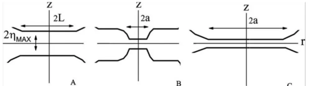
1.1. Schematic picture of the system

Consider two identical large vesicles brought in the initial state at the equilibrium distance

D

_(Fig.1).

Fig 1 Energy profile vs distance

Typically, the energy-distance curve exhibits two minima: a shallow long-distance minimum (the so-called secondary minimum) at

z

=

D

_{and a}

deep short-distance well at MAX

D

z= −2η _{(the primary minimum).}

The energy-distance curve arises from different contributions.

The classical DLVO theory19 of colloid particles considers a combination of repulsive electrostatic forces and attractive van der Waals interactions. Their combination may give rise to an energy double well profile. In biological membranes other contributions must be accounted for. For instance, the strongly hydrophilic membrane surface induces overwhelming short-range repulsive hydration forces due to water ordering at polar interfaces20,21

Besides, long-range repulsion forces arising from the protruding hydrophilic sugar residues of glycolipids and glycoproteins22 _{have to be considered. At short distance, the}

repulsive forces are generally stronger than the dispersion ones. However, specific molecules may form tight ligand-receptor bonds between nearby membranes yielding a sharp minimum at distances comparable with the ligand size23 (Fig.1). A common biomimetical system is the biotin-streptavidin couple, but also simple divalent cations are effective in bridging negatively charged membranes.

A cartoon of the process is given in Fig.2 where the evolution from loosely bound (left) to tight bound (right) large vesicles via the formation of a localised dimple is reported.

Fig 2 Evolution from loosely bound (left) to tight bound (right) large

For simplicity only the vesicles adhesion region has been drawn. The contact area of strongly (left) and weakly (right) bound states appreciably differs, the

weakly bound state depending on the adhesion energy and vesicle radius is much greater than the critical adhesion plaque radius

The mechanism sketched above

→_{short-distance transition of “soft” particles.}

and/or their size is large, this route is an efficient alternative to the undeformed approach mechanism (DLVO theory) still valid in modelling adhesion/fusion kinetics of very small vesicles

The picture described so far accounts for early stages of the fusion process that may further evolve through more steps. Let us consider in detail the

process among vesicles V

The first reversible step second one

tight loose

V

V₂ → ₂

approaching the undeformed membranes (as in the DLVO theory) or via a dimple formation like in the present model.

followed by a displacement of the lipid polar headgroups giving rise

patches. They attract each other until the external part of the contacting membrane bilayers merge forming a stalk.

... ...

2

1 →T → Tn →

T

, can be thought as a cascade of

merging of the tight adhering membranes into a new bigger vesicle Evolution from loosely bound (left) to tight bound (right) large vesicles

For simplicity only the vesicles adhesion region has been drawn. The contact area of strongly (left) and weakly (right) bound states appreciably differs, the

weakly bound state depending on the adhesion energy and vesicle radius is much greater than the critical adhesion plaque radius a*_.

The mechanism sketched above suggests an alternative route for the long

distance transition of “soft” particles. When the particles rigidity is small and/or their size is large, this route is an efficient alternative to the undeformed nism (DLVO theory) still valid in modelling adhesion/fusion kinetics of very small vesicles25

The picture described so far accounts for early stages of the fusion process that may further evolve through more steps. Let us consider in detail the

V _:

The first reversible step

loose

V V

V + ⇔ _{2 is diffusion-controlled} tight

is slow and basically irreversible. It may occur either by approaching the undeformed membranes (as in the DLVO theory) or via a dimple formation like in the present model. The transition to the short-distance minimum is followed by a displacement of the lipid polar headgroups giving rise

patches. They attract each other until the external part of the contacting membrane bilayers merge forming a stalk. Stalk formation and evolution,

, can be thought as a cascade of N intermediates describing the merging of the tight adhering membranes into a new bigger vesicle

5

vesicles (adapted from 31)

For simplicity only the vesicles adhesion region has been drawn. The contact area of strongly (left) and weakly (right) bound states appreciably differs, the size

L

_{of the}

weakly bound state depending on the adhesion energy and vesicle radius24, in any case

L

suggests an alternative route for the long-distance When the particles rigidity is small and/or their size is large, this route is an efficient alternative to the undeformed nism (DLVO theory) still valid in modelling adhesion/fusion

The picture described so far accounts for early stages of the fusion process that may further evolve through more steps. Let us consider in detail the whole fusion

controlled, while the . It may occur either by approaching the undeformed membranes (as in the DLVO theory) or via a dimple distance minimum is followed by a displacement of the lipid polar headgroups giving rise to hydrophobic patches. They attract each other until the external part of the contacting membrane Stalk formation and evolution, →

tight

V₂

intermediates describing the merging of the tight adhering membranes into a new bigger vesicle

P

. The

6 structure of the different fusion intermediates (stalk, hemi-fusion, pre-pore and connecting pore) has been postulated and/or observed.

In some cases, the short-distance adhesion might be the bottleneck to the whole fusion process because of the lateral tension developing in strongly adhering vesicles26. At tight adhesion, the tension is so strong that membranes destabilization and fracture is likely when they are stretched beyond a critical value27 _{(lipid membranes cannot be}

stretched beyond 2-4% without rupturing28. In other cases, vesicles strongly adhere but do not fuse because of the high energy of the stalk. In any case, the formation of tight adhering membrane patches is a fundamental step in the fusion process. The well-known fusogenic behaviour of hydrophilic polymers can be understood in term of enhanced adhesion, while it is hard to conjecture that the stalk energy, mainly related to the structure of the membrane inner core, is modified by polymer dissolved in the aqueous phase.

We focus on the initial process V +V ⇔V2loose→V2tight.

1.2. Formation energy of an adhesion patch

1.2.1. Bending Energy

Following Helfrich29 the bending energy of an isolated elastic membrane is

∫

      + − + = S G o M bend K C C C K C C dS E 1 2 2 2 1 ) ( 2 1

, where C1 and C are the principal 2

curvatures, Co the spontaneous curvature (Co =0 for planar membranes), KM is the bending rigidity per unit area and KG the elastic modulus of Gaussian curvature. The integration is extended over the whole membrane surfaceS_{. The elastic constants} KM and KG can be obtained from experiments or predicted from the membrane structure.

Typically30 KM ≈ erg

12

13 ₁₀

10− ₋ −

7 undergoing local deformations ηA and ηB, in the Helfrich approximation we re-write the above equation as dxdy y x y x K y x K E _M j j _G j j j S S B A j bend o                     ∂ ∂ ∂ − ∂ ∂ ∂ ∂ +             ∂ ∂ + ∂ ∂ =

∑

∫∫

> = 2 2 2 2 2 2 2 2 2 2 2 , 2 1 η η η η η ( 1 ) The integration is extended outside the adhesion site, S>So, while in the region o

S

S < _{the bending energy is zero because the adhesion plaque is planar.}

1.2.2. Interaction energy

The bending energy must be supplemented by the repulsion energy between the membranes. As said before, in the initial state the membrane stays in a shallow long-distance minimum (Fig.2, left panel). On approaching the membranes along their perpendicular z−_{axis the energy first increases, thereafter it falls inside a short-distance}

minimum (Fig.1). Adopting a phenomenological picture, we approximate the membrane-membrane interaction outside the plaque (S>So) by a quadratic function of the

deformation:

∫∫

> − = o S S B A rep F dxdy E ( )2 2 1 η η

. The coefficient

F

_{can be derived from}

experimental measurements or predicted from the membrane structure. Inside the plaque (S<So) the deformation takes its largest value (ηA(x,y)=−ηMAX ,ηB(x,y)= +ηMAX ),

then the above formula reduces to Erep F MAX So

2 ) 2 ( 2 1 η =

. Combining the two terms

        − + =

∫∫

>So S B A o MAX rep F S dxdy E 4 2 ( )2 2 1 η η η ( 2 )

8 1.2.3. Bridging energy

Inside the adhesion disk the membrane distance is short enough to allow the formation of Cis complexes tightly joining the opposite membranes. The bridging energy is written as Ebridge = −ECσCθCSo ( 3 )

where −EC is the sticking energy per complex,

σ

C the two-dimensional stickers concentration, So the adhesion plaque area and 0<

θ

C <1 the fraction of stickers that form Cis complexes.

Adding together contributions (1)-(3) ETOT = (2F MAX −EC C C)So+ 2 θ σ η         +       ∂ ∂ ∂ − ∂ ∂ ∂ ∂ +       ∂ ∂ + ∂ ∂ +       ∂ ∂ + ∂ ∂

∫∫

> 2 2 2 2 2 2 2 2 2 2 2 2 2 2 2 2 2 2 1 y x y x K K y x y x K A A A M G B B A A S S M o η η η η η η η dxdy K F y x y x M A B B B B     − +           ∂ ∂ ∂ − ∂ ∂ ∂ ∂ 2 2 2 2 2 2 2 ) (η η η η η ( 4 )

After some algebra given in ref.31 enabling us to express the optimized adhesion energy as a function of the adhesive disk radius a, Excess(a)≡ETOT(a)-EFLAT

(defined as the difference between the energy of the patch-forming membranes and that of the flat membranes at equilibrium distance), we find to the leading term:

E

EXCESS₌ A A a A1a 2 3 2 ) ( 2 1 + − µa>>1 _{( 5 )}

where: A2 ≡ 4πFηMAX2 ;A3 ≡ 2πEσCθC;A1 ≡ π27/4ηMAX2 F3/4K1M/4;B ≡

2 / 1 2 / 1 2 2 / 7 2 ηMAXF KM .

For that concerns biological membranes, when µa>>1 _{, the membranes pay a} huge energy cost to form an adhesion site. On the contrary, the less common case describes either slightly repelling membranes or extremely tight ligand-receptor bridges, where we may suppose the adhesion site to be pointlike.

It is worth discussing the energy behaviour. The first term of eq.(5),

2 3 2 2

1_{(A −A )a}

, accounts for the balance between adhesion and repulsion forces inside the adhesion disk, while A₁a _{describes the energy outside the disk. The linear dependence}

9 on a _{means that the elastic energy is located in a narrow strip around the disk periphery.} When A2 −A3 >0 _{(repulsive energy greater than adhesion), the energy monotonously}

grows with

a

, but when A2−A3 <0 _{(repulsive energy smaller than adhesion) the}

energy first reaches a maximum, then decreases (fig.3). In this nucleation process only nuclei bigger than a critical size further grow until full membrane adhesion is attained. The non-equilibrium concentration of the critical nuclei is calculated in the forthcoming section.

Fig. 3 Energy profile whenA2−A3 <0 _{(repulsive energy smaller than adhesion).}

1.3. Nucleation rate

Sudden ligand-receptor bridging (x→∞)

According to the classical non-equilibrium theory of nucleation processes, the time evolution of the nuclei distribution P( ta, ) in the space of nuclei size a _satisfies the continuity equation32

a J t P ∂ ∂ − = ∂ ∂ (6)

where J ≡ J( ta, ) _{is the flux of nuclei going from the size a to a+da.}

a*

10 The flux arises from competing condensation and dissolution processes, acontinuum picture yields

) / ( ) ( ) , ( eq P Peq a P a D t a J ∂ ∂ − = (7)

where the equilibrium distribution is: Peq(a)=Poexp

(

−Φ(a)/kT

)

. Po defines the concentration of the smallest nuclei (embryos) and Φ(a) is the minimal work needed to form a nucleus of radius a_{. We may identify} Φ(a) ₌EEXCESS, this latter being the energy of two nearby membranes connected through an adhesion patch given by eq.(5). D (a) plays the role of a “diffusion coefficient” in the space of nuclei sizes.

A compact expression for the steady rate of nuclei production is:

S J _≈     Φ         ∂ Φ ∂ − = kT a a kT a D P a a o *) ( exp 1 *) ( 2 1/2 * 2 2 π ₍₈₎

The model developed so far describes most nucleation processes like the formation of a solid from a fluid phase. Nevertheless, the adhesion/fusion process requires specific models to calculate:

a) The activation barrier to membrane adhesion Φ(a) which depends on the balance between adhesion forces, compression energy and bending energy.

b) The “diffusion coefficient”D (a), a measure of the adhesion plaque growth rate, is related to the membrane fluctuations near the plaque rim. It depends on viscous and elastic forces as well.

c) The probability Po to form the smallest embryos (a→0) which is all but nothing the collision probability between nearby fluctuating membranes.

Noninstantaneous bridging kinetics (χ → 0)

In the other relevant limit χ → 0 (extremely slow bridging kinetics) the number of bridges remains very small during the plaque growth preventing the formation of stable adhesion sites, thus limχ→0JS ≈0 _{( 9 )}

11

1.4. Results and discussion

By hypothesizing that the short-distance adhesion is the bottleneck to the whole fusion process, one may apply the model to rationalize real fusion events.

a) When large vesicles are considered, the model valid for deformable bodies predicts that the barrier to adhesion is independent of vesicle radius R . This result is in sharp contrast with the adhesion models of rigid spheres where the rate exponentially decreases with radius19 _{Therefore, cell-sized objects would never fuse together}

because R is too large.

b) According to our model for adhesion to occur a critical ligand concentration must be attained. Afterwards, the adhesion rate remains sensitive to the concentration c¯ of divalent cations bridging two negatively charged lipids. The following equation:

            >         − − >           − − < ≈ + _ _ 2 1 _ _ 2 / _ 1 _ ' exp exp 0 c high c c C E C c small c c C Ee c C c c rate crit crit kT E crit ( 10 ) evidencing a burst of the adhesion rate above a critical ion concentration.

c) The model highlights a strong sensitivity of the fusion rate on the bridging energy E and therefore a great ion specificity (at variance of DLVO theories). Experimentally, the ion specificity has been well established long time ago33 . It is worth mentioning the dramatic difference between Ca2+ and Mg2+, calcium being much more effective in triggering and enhancing the fusion rate.

d) The adhesion rate sharply decreases with the membrane repulsion F roughly as:

        − − ≈ F C F const rate 1 exp 2 / 3 .

12 High F are likely in charged membranes, but also neutral phosphatidylcholine (PC) vesicles, the most abundant component of living cells membrane, exhibit large F because of the overwhelming hydration forces20,21,34,35,36. This fact explains way PC vesicles do not spontaneously fuse, unless we consider strongly strained small unilamellar vesicles37 or vesicles squeezed together by depletion forces38.

e) For planar membranes approaching along their perpendicular axis, the long-distance

→ short-distance transition probability increases with the bending rigidity K . This M is due to the lowering of the undulation forces39 _{great at small K (M} ≈T2/K_M).

Conversely, in our model: rate≈exp

(

− const KM1/2

)

, showing a decrease of the adhesion with K . The effect, however, is weaker than that found by increasing the M repulsion F . Experimentally, the fusion rate is faster when the membrane is in the fluid phase (low bending rigidity) than in the gel phase where the bending rigidity is up to an order of magnitude higher40.

f) A pressure ℑ applied to the adhering membranes (e.g., osmotic forces induced by water soluble polymers sterically excluded from the inter-vesicles space, usually named as depletion forces) reduces the equilibrium interlamellar distance.

g) The temperature behaviour of the adhesion rate depends both on direct

(rate≈exp(−const /T) and indirect effects, these latter being related to the thermal variation of physical parameters. Among the indirect effects we mention the lowering of membrane rigidity above the thermotropic gel→_{fluid phase transition, often} accompanied by an increase in the fusion kinetics. Typically, fusion rate increases with T , with a sharp maximum near the membrane transition temperature T°41

h) An intriguing result is the behaviour of the fusion rate with solvent viscosity

ω

. Indeed, the nucleation kinetics depend on the balance between plaque growth v (proportional to 1/

ω

) and dissolution rates. Below a critical size, the dissolution rate

13 depends on the bridges concentration. In viscous fluids the longer life time of the adhesion enables the formation of more bridges with a consequent lowering of the “dynamic” barrier.

i) Adhesion is faster at high ligand-receptor bridging rateχ . In order to form Cis complexes, the charged lipids belonging to opposite membranes must diffuse along the membrane surface and encounter.

The model developed so far does not describe the truly fusion process (the merging of the two contacting membranes with the formation of an expanding pore). This fusion process has been fully investigated by other authors42 and it will not investigated in our thesis. Notwithstanding, the model addressed in the previous section (the formation of an ion-assisted stable adhesion plaque at contact distance, or, in biochemical language, the “de-hydration” step) probably accounts for the true kinetic transition state of the whole fusion process. This is a consequence the high energy required to form a local protrusion of a lateral critical size.

The overall fusion rate, however, do depend both on the transition state energy barrier, but it is also related to the number of weakly-adhering vesicles pairs contained in the sample. Most of the forthcoming calculations will address this relevant topic. They will describe the well-known polymer effect on the adhesion energy between two identical flat charged membranes set at equilibrium distance. The results will compared with the behaviour of neutral membranes.

14

2. THERMODYNAMICS OF THE PSEUDO-TERNARY SYSTEM

POLYMER+IONS+ SOLVENT

Before to investigate the polymer effect on a pseudo-ternary solution that contains solvent (water), ions and a neutral but soluble polymer. The mixing behavior of this ternary system is not trivial at all. Its properties will for the basis for understanding the polymer effect on the adhesion of charged membranes embedded in a polymer solution.

Let us begin by considering a dilute aqueous electrolyte solution in which a neutral polymer of lower dielectric permittivity is dissolved. We define c±(r) to be the

local dimensionless concentrations of positive and negative single-valent ions, each of them carrying a unit charge

±

e

, and cZ+(r) as the concentration of multi-valent ions of

valence Z . In biological systems, + c±(r) is typically ~10-1 M while cZ+(r) (mainly

Z=2) is about 10-6 M . We require, that the average concentrations (ci) of the different ions must satisfy the electroneutrality condition

Z M

Z c c Z c

c

c+ + + + − =2 +( + +1) ( 11 )

where cM and cZ are the macroscopic concentrations of monovalent and Z-valent salts, respectively. We define Φ(r) to be the local polymer volume fraction,

_

Φ the average polymer volume fraction and N _{the degree of polymerisation. In the}

following, we will explore the physically relevant case of semi-dilute polymer solutions defined over the concentration range 1

_ 5 / 4 << Φ << −

N 43_{. In this range, the polymer coils} overlap but the polymer fraction is still low. This is a situation that allows for a continuum treatment of polymer solutions. At lower concentrations (dilute regime), coils behave like an ideal gas of isolated spheres of the radius RG( N≈ 3/5). The energy of the polymer solution is the sum of contributions coming from polymer and electrolytes. We describe these contributions next.

15

a) Polymer contribution

In a mean-field picture the free energy of a polymer solution can be written as44,45 = POL E 

(

)

 Φ ∇ Φ − Φ

∫

2 2 3 _{24 (r)(1 (r))} (r) a a kT V + Φ Φ + N N ) ( log ) (r r + Φ − Φ − ( ))log(1 ( )) 1 ( r r χΦ(r)(1−Φ(r))   dV _{( 12 )}

where k _{is the Boltzmann constant and}

T

the absolute temperature. a _{denotes the} diameter of a single molecular unit (monomer, ion and solvent) that, for the sake of compactness, are assumed having the same size.

The first term accounts for the energy loss associated to spatial heterogeneities. In polymer solutions, perturbations due to chain-interface boundaries propagate deep inside the fluid. This is at variance with molecular fluids consisting of small molecules where the concentration gradients are localised near the interface. The remaining two terms in (12) describe the homogeneous component of the polymer energy in the Flory-Huggins approximation43. The second and third terms describe the polymer and the solvent mixing entropies. Strictly speaking, the solvent contains both solvent molecules and different kinds of ions (monovalent anions and cations and a small amount of Z-valent cations), but in semi-dilute solution we may safely assume:

) ( 1 ) ( ) ( 1 ) (r = −Φ r − r ≈ −Φ r Φ

∑

i i s c

. The fourth and final term accounts for the polymer-polymer, polymer-solvent and solvent-solvent interactions as described by the mean-field Flory interaction parameter χ =χ(T). The contributions arising from polymer-ion and solvent-ion interactions is added in the following section b.

b) Electrolyte contribution

The good solubility of ions in a melt of hydrophilic polymers is well-known46.

This property constitutes the basis of several technological applications such as electrolytic fuel cellsErrore. L'origine riferimento non è stata trovata.. On the other hand, in polar solvents, e.g. water, ions prefer more polar environment47. _{When the solvent}

16 polarization energy overcomes the entropy of mixing (low in polymer solutions because of chain connectivity), ions induce phase separation of homogeneous water/polymer mixtures and the formation of fluid phases.

In order to describe the contribution of the electrolyte in the ternary polymer + solvent + electrolyte system, we decompose the energy of the ions into a sum of two main terms:

i) A standard entropic contribution that for dilute electrolyte solutions takes the simple form:

dV c c c c c c a kT TS Z Z V

ION = 3 ( ( )(log ( )−1)+ ( )(log ( )−1)+ ( )(log ( )−1))

−

∫

₊ r ₊ r ₋ r ₋ r ₊ r ₊ r

ii) The solvent interaction contribution. In homogeneous fluids, the ion-solvent energy of an interaction can be calculated as a function of the fluid dielectric permittivity ( )

_

Φ ≡ε

ε _{and the electrolyte concentration}

c

_{. For a single ion of radius r,}

standard electrostatics yields a Born-like equation48: E_SOLV = _

    + − − ) 1 ( 1 1 2 2 2 r r e Z κ ε _,

where Ze _{is the ion charge and}

2 / 1 3 2 2 _/ 8       ≡ e

∑

Zici a kT i

ε

π

κ

is the inverse of the Debye length (the a−3 _{term appears because we use dimensionless concentration}

c

_{). In a cell} system where solvent and monomers have identical size, the ion radius r and cell size length a are trivially related:34πr3 =a3. Moreover, since

1

10− ≈

r

κ _{at physiological salt} concentration, we may approximate (1+κr)−1 ≈1−const⋅c1/2.

The above formula can be generalised to include a spatially inhomogeneous ion distribution. Up to terms proportional to O(c±3/2(r)), we obtain:

= SOLV E _{a a z} c z c z Z c z dV e Z V )) ( ) ( ) ( )( )) ( ( 1 1 ( ) ( 2 2 3 3 / 1 3 4 2 + + − + + + Φ − −

∫

ε π , where c±(r)

and cZ+(r) are local ionic concentrations. We have neglected the ion-ion interaction

energy given that it is proportional to O(c3±/2(r)). To a good approximation, the local

dielectric permittivity of a fluid can be described as the weighted average of solvent (

ε

s) and polymer (εp) permittivities

17 ) ( )) ( 1 ( )) ( (Φ r ≈ε_s −Φ r +ε_pΦ r ε ₍₁₃₎

This empirical formula has been experimentally verified for several water-polymer mixtures, including PEG solutions49,50,51,52. At low polymer concentrations it is consistent with the Maxwell-Garnett theoretical equation53,54.

Adding together the two above contributions, −TSION and ESOLV, we get a

simple formula for the electrostatic energy term of a dilute electrolyte solution

[

− + − + − −

= 3

∫

+(r)(log +(r) 1) −(r)(log −(r) 1) Z+(r)(log Z+(r) 1))

V ELECT c c c c c c a kT E

]

dV c Z c c B )( ( ) ( ) _Z ( )) )) ( ( 1 1 ( 2 r r r r + + − + + + Φ − ε _{( 14 )} with akT f e B 2 ) ( 1/3 3 4 2 _π ≡

, where f>1 is an empirical parameter that takes into account dielectric saturation effects near a strongly charged electrolyte surface55. This effect reduces the numerical value of the dielectric permittivity near the ion and, whence, the ion solvation energy. Other specific effects, such as the deviation of the ionic radii from the averaged molecular size a, can be also included into f. It is worth noticing that in (14) the coupling between polymer, solvent and electrolytes is related to the ion solvation energy through the variation of the dielectric permittivity with polymer concentration. Combining equations (12) and (14), the total energy is the sum of a polymer and

electrolyte contribution ELECT POL

TOT E E

E = + _{( 15)}

Ternary system stability

The response of a pseudo-ternary polymer+ions+solvent solution to small thermally-induced fluctuations of polymer and electrolyte concentration can be written as: Φ(r)=Φ+

δ

Φ(r), ci(r)=ci +

δ

ci(r). We inserted these expressions into (12)-(15) to

develop the total free energy as a function of the amplitudes δΦ(r) and

δ

ci(r) up to quadratic terms. We describe fluctuations as a linear combination of sinusoidal waves:

18 r q r q o q ⋅ Φ = Φ( )

∑

δ sin δ and r q r q o q ⋅ =

∑

sin ) ( i, i c c δ δ

. Integrating over r, the linear terms vanish and we obtain

+ = o TOT TOT E E         Φ + + Φ _Φ Φ Φ

∑∑

∑

∑

o c c j j o j c c j j o j j j j c c A c A A a kTV q o q o q q q q , ,' , ' 2 3 ( ) ' 4 δ δ δ δ δ ( 16 )

The coefficients A are easily found with the aid of the electroneutrality jj'

condition (11): ) ) 1 ( 2 ( ) ( ) ( 2 2 1 1 1 ) 1 ( 24 3 2 2 2 Z M s p c Z Z c B N q a A + + Φ − − − Φ − + Φ + Φ − Φ = _{+ +} Φ Φ _ε ε ε χ M c c c A = 1 + + , M Z c c c Z c A + + = − − 1 , Z c c c A_{Z Z} = 1 + + = + Φc A = − Φc A 2_(Φ) − − ε ε ε_{p s} B , AΦcZ+ = ( ) 2 2 Φ − − ₊ ε ε ε_{p s} B Z , Ac+c− = Ac+cZ+ = 0 = + −cZ c A

The system is stable against concentration fluctuations when det A >0. The condition det A =0 defines the so-called spinodal curve that divides the phase diagram into stable and unstable regions. Focusing our attention onto macroscopic phase separation, q → 0, we obtain 0 ) ( 2 1 1 1 = Φ − Φ − + Φ eff N χ _{( 17 )}         = − Φ + − Φ − + = − Φ Φ − + = Φ + + + + 1) 0 ) ( 2 ) 1 (( ) ( ) ( ) 1 ( 0 ) 1 ) ( 2 ( ) ( ) ( 2 ) ( 2 3 2 3 2 M Z s p Z M s p eff c c B Z Z Z BZ c c B B ε ε ε ε ε ε ε ε χ χ ( 18 ) Equation ( 18 ) shows that multi-valent ions are more effective in inducing phase

19 separation. Figure 4 shows the spinodal curve as a function of the Flory interaction parameterχ = χ(T) calculated at different monovalent, cM, or multi-valent, cZ, salt concentrations.

Fig-4 Phase diagram for a polymer-solvent system in the absence (full line) and in the presence (dashed

lines) of a constant salt concentration . Curve a) refers to a 0.15 M salt formed by both monovalent anions and cations. Curve b) refers a 0.15 M salt formed by monovalent anions and divalent cations. The sizes of anions and cations were assumed to be identical. In the region below the curves the polymer is homogeneous, while above the curves the system phase separates. Setting N=100 and χ ≈0.49, we find that that the fluid becomes unstable to concentration fluctuations in the presence of divalent ions.

We can now make the following conclusions from our simple model:

a) upon increasing the salt concentration (c or M c ), the compatibility between a Z soluble non-ionic polymer and a polar solvent becomes worse56,57_.

b) the ion effect is larger when solvent and polymer have strongly different dielectric permittivity.

c) Z-valent ions (neutralized by mono-valent counter-ions) are much more effective (about one order of magnitude) than single-valent ions. Experimental data show that trivalent ions, like citrate or phosphate, easily induce phase separation in aqueous polymer solutions51,52.

d) By maintaining constant ion charge but varying the radius, it can be easily seen that small ions are more effective than big in inducing polymer phase separation (this effect is contained in the coefficient −1

∝a

B _{). This is in qualitative agreement with} experiments51,52_.

N

χ

Φ

a

20

3. POLYMER EFFECT ON THE ADHESION/FUSION RATE

3.1 Art state on PEG-mediated fusion:

Several mechanisms were suggested for how PEG accomplish the fusion process, including: increasing surface tension, absorbing to and crosslinking bilayers, altering the structure and dielectric properties of bulk water, altering the molecular order of the bilayer at the point of contact, producing volume-exclusion-induced aggregation and dehydration, induction of non-bilayer structures, acting as a detergent to disrupt bilayer structure, inducing phase separation that destabilizes the bilayer, producing compressive and then, upon dilution, expansive osmotic stress on membrane vesicles, and containing impurities that disrupted membranes. These proposals and their origins were previously reviewed in detail58_{. PEG was known to aggregate membranes, as}

demonstrated quantitatively by electron microscopy59 _{and X-ray scattering}60_{. Some}

explained this according to surface absorption and cross-linking. Arnold showed that low molecular weight PEG covalently attached to an alkyl chain that would insert into bilayers, pushed bilayers apart61_{, rather than drawing them together. This suggested that}

absorption of PEG to membrane surfaces was not likely to explain PEG-mediated membrane aggregation, as was confirmed by the observation that PEG could be separated from lipid vesicles by a dialysis membrane and still drive membranes into closer contact60.

In addition, Arnold demonstrated that water was excluded from regions of contact between PEG aggregated vesicles using NMR62 and electrophoretic mobility63.

A theoretical treatment supported these experiments by showing that surface exclusion would be expected to provide a membrane aggregating attraction64_{, as was then confirmed}

by direct experiment65_{. Today we know that, aside from producing a thermodynamic}

force driving close contact between membranes, PEG also promotes fusion via a positive osmotic pressure that likely helps stabilize fusion intermediates66. The main

effect of PEG on membrane vesicles is believed to be a volume- exclusion aggregation of membranes and dehydration in areas of contact.

21

3.2. Establishing new aspects of peg-mediated fusion

Consider two identical large vesicles brought at distance

D

_{as shown in}

Fig.1. When their radii are large, we may neglect curvature effects and consider two parallel surfaces. Classical DLVO (Derjaguin-Landau-Verwey-Overbeek) theory of colloids67considers a combination of repulsive electrostatic forces and attractive van der

Waals interactions. In biological membranes, other contributions must also be accounted for. For instance, the strongly hydrophilic membrane surface induces short-range repulsive hydration forces due to water ordering at polar interfaces35,36,68,69,34 and at short distances ligand-receptor bonds may be formed between certain membrane proteins1,2,3,4 or even by simple divalent cations5.

We consider the effect of uncharged soluble polymers and focus our attention on the screened electrostatic forces associated with the membrane surface charges. Other forces (like van der Waals and hydration ones) are rather insensitive to polymer addition, constituting a constant background that will be separately added to the total energy.

The system interchanges matter with an external infinite reservoir and after equilibration, the inter-membrane space and the bulk reach different polymer and electrolyte compositions. For the sake of simplicity, we restricted our analysis to temperatures and concentration ranges (low salt and polymer concentrations) , see section 2 ensuring in order avoid any phase separation of polymer and solvent in the bulk fluid. components do not phase-separate. We considered only laterally homogeneous membranes.

Letting r= z be the distance of a generic point inside the inter-membrane gap from the membrane surface and

D

_{to be the gap width, the free energy in the gap region}

can be partitioned into bulk and surface contributions. Part of the contributions is outlined in the previous section and new contributions will derive by the broader framework that includes the presence of membranes.

a) Bulk contribution

22 a) an energy term related to the electrostatic interactions between the electrolyte’s charge distribution and the electrostatic potential:

= ) ( ) (rψ r ρ (e/a3)(Z₊c_Z+(r)+c₊(r)−c₋(r))

ψ

(r) _and

b) an energy loss (per unit volume) due to the gradient of the electric field: 8 ( ) 2( )

1_{ε r E r}

π −

, where E(r)= −∇ψ(r) _{is the electric field and} ε(r)≡ε(Φ(r)) _{the dielectric permittivity} of the fluid mixture given by ( 13 ).

Adding the two terms and integrating over the inter-membrane space, we have

[

a Z c c c

]

dV e EFIELD _V ( ( ))( ( )) 3 ( Z ( ) ( ) ( )) ( ) 2 81πε Φ r ∇ψ r + + + r + + r − − r ψ r − =

∫

( 19 ) The local ion densities ci(r) and the potential ψ(r) must be calculated self-consistently.

b) Surface contribution

At the membrane-solution interface (z = 0) the free energy contains additional terms:

a) a term describing the interaction between the charged lipid heads and the surface

potential: b e z dS X

z

S 0

2

∫

ψ( ) =

, where X is the (charged lipids)/(total lipids) fraction, b is 2 the surface area of a lipid and e the unit charge (σ =eX / b2 _{defines the membrane’s} charge density),

b) a term accounting for the interfacial energy of the polymeric solution dS z a z S 0 2 ( ) 1 = Φ

∫

γ

,

γ

being the polymer-membrane adhesion energy. Combining these

two gives ESUP ≈

[

2 a S 0 2 _{( )} ) / (a b Xeψ z _z= + Φ( ) ₌₀

]

z z γ _{( 20 )}

Next, we combine volume and surface energies and introduce a new variable to describe the polymer volume fraction

) ( ) ( 2 z z =Φ

τ

_{( 21 )}

23 = S E_TOT/ 2

[

1 a 0 2 2 _{/ ) ( )} ( ₌ z z Xe b a ψ 2_{( ) 0}

]

= + z z τ γ ₊ + +          ∂ ∂

∫

( ) ( ( )) 6 2 2 2 / 0 3 F z z z a a kT FH D τ τ ) 1 ) ( )(log ( ) 1 ) ( )(log ( + − + − − − + z c z c z c z c ) 1 ) ( )(log ( − +cZ+ z cZ+ z +       ∂ ∂ − 2 3 _{( )} )) ( ( 8 z z z kT a ψ τ ε π ) ( )) ( ) ( ) ( (c z c z Z c z z kT e Z+ ψ + − + − + dz z c Z z c z c z _{Z }   + + Ω − (ε(τ( )))( ₊( ) ₋( ) ₊2 ₊( )) ( 22 ) where FFH( zτ( )) is the Flory-Huggins component of the polymer energy:

≡ )) ( ( z FFH τ )) ( 1 )( ( )) ( 1 log( )) ( 1 ( ) ( log ) ( 2 2 2 2 2 2 z z z z N z N z τ χτ τ τ τ τ − + − − + , and       − ≡ Ω )) ( ( 1 1 ))) ( ( ( z B z τ ε τ ε .

Inside the gap, electroneutrality imposes a slight charge excess of electrolyte solution to balance the surface charge density σ =eX / b2_{. Hence, the concentrations}

) (z

cj must satisfy the constraint

(

)

b X e dz z c z c z c Z a e Z D 2 2 / 0 3

∫

+ +( )+ +( )− −( ) = ( 23 )

The equilibrium distribution of the different species is attained when their chemical potentials are identical both in the gap and in the reservoir. This implies a constrained energy minimization procedure as outlined in Appendix A. Specifically, variation of the total free energy with respect to ci(z) gives

0 ))) ( ( ( ) ( ) ( log _± ± ψ z −Ω ε τ z −µ_± = kT e z c ( 24a ) 0 ))) ( ( ( ) ( ) ( log _{+ −} 2_{Ω − =} + + + + Z Z z Z z kT e Z z c ψ ε τ µ ( 24b )

24

j

µ _{being undetermined Lagrange multipliers. Since these relationships must be} valid independent of z, we set z → ∞ _{(bulk solution). Recalling that:} limz→∞ψ(z) =0,

j j

z→∞c (z)=c

lim

, and limz→∞ε(τ(z))=ε , we can easily calculate the Lagrange’s multipliers j

µ _{. The final result reads}

(

)

      ∆Ω = _± ± kT z e z c z c ( ) exp (

τ

( )) exp m

ψ

( ) ( 25a )

(

)

      − ∆Ω = + + + + kT z e Z z Z c z cZ Z ) ( exp )) ( ( exp ) ( 2 ψ τ ( 25b ) ±

c and cZ+ being the ion concentrations in the bulk and

      − ≡ ∆Ω )) ( ( 1 1 )) ( ( z B z τ ε ε τ

. Lastly, minimization of H with respect to τ(z) and ψ(z), together with use of explicit expressions for ε( zτ( )) (eq.(13)) and ci(z) (eqs.(25)), yields a pair of coupled differential equations. By introducing dimensionless potential and polymer concentrations ψ*=eψ(ς)/kT _,

τ

*=

τ

(

ς

)/Φ1/2 _{and dimensionless distance}

a z/ =

ς _{, the final equations read}

(

( *) ( *, *)

)

* 0 6 * 1 2 2 = + + ∂ ∂ τ τ ψ τ ς τ G Go (26a )

(

*

)

sinh *) ( 1 1 exp * *) ( 2 2 ψ τ ε ε κ ε ς ψ τ ε ς _            − =       ∂ ∂ ∂ ∂ B a ( 26b )

where

κ

≡

(

8

π

e2c/a3

ε

kT

)

1/2 is the Debye length of a homogeneous mixed solvent and * log 2 ) 1 * ( 2 1 * 1 log *) ( 2 2 0 χ τ τ τ τ N G _+ Φ − −      Φ − Φ − ≡ ( 27a ) The term

25

[

( )

]

_       −               − +       ∂ ∂ − ≡ cosh * 1 *) ( 1 1 exp *) ( 2 * 8 ) ( *) *, ( _{2 2} 2 2 2 1 ψ τ ε ε τ ε ε ε ς ψ π ε ε τ ψ Bc B e akT G p s M (27b ) describes the is a coupling term between the electrostatic potential and polymer

concentration. Specifically, the gradient term in (27b) is related to the dielectric inhomogeneities of the medium, while the B- dependent term describes salting-out effects linked to the different solvent and polymer dielectric permittivities. The salting-out effect appears also in the second term of the right-hand side of equation (27b).

In (27b) we disregarded terms depending on cZ+(ς). Despite the relevant role

of multivalent ions in screening the electrostatic potential, the ratio between the mono- and divalent ion concentration in biological fluids is as small as 10-5, enabling us to neglect the role of cZ+(ς) on ψ * and

τ

*. This approximation, however, is no longer

permissible at the membrane-water interface ς =0 because of the large binding constant of multi-valent ions with charged membranes. This point will be thoroughly discussed in the next section where the effect of bound ions on the electrostatic and polymer profiles will be investigated.

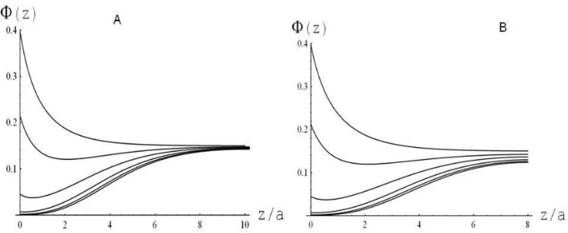
With (26a) we can calculate the inhomogeneous polymer distribution

2 * )

(

ς

=Φ

τ

Φ _{. If we omit in (26a) the ion-polymer coupling term} G1(ψ*,τ*) , in (27a), develop the Flory-Huggins polymer energy up to _*4

τ _{and neglect the small term} proportional to −1

N , we recover the de Gennes equation for the concentration profile of a semi-dilute polymer near a wall43: (1 * ) * 0

* 2 2 2 = − + ∂ ∂ τ τ ς τ A , with A≡6(1−2

χ

)Φ. Equation (26b) is nothing but a generalized Poisson-Boltzmann equation and at constant polymer concentration (

τ

*→1) it reduces to the familiar expression:

(

*

)

sinh * 2 2 2 ψ κ ς ψ = ∂ ∂ .

The above equations must satisfy proper boundary conditions. In the case of two identical surfaces, (4Ab) of Appendix A gives

26 More interesting is the behaviour of ψ * and τ * at the interface ς =0. From (4Aa) we get X b a kTa e2 2 0 0 4 * ) * (       = ∂ ∂ ⋅ = = π ς ψ τ ε ς ς ( 28b ) 2 / b eX =

σ _{being the membrane surface charge density. Analogously, from (4Aa)} we obtain a boundary to the polymer profile at ς =0

0 0 * 6 * = = = ∂ ∂ ς ς τ γ ς τ kT _{( 28c )}

a formula connecting the interfacial polymer concentration to the adhesion energy

γ

_{. The differential equations (26a,b), subjected to the boundary conditions (28a-c), are} the basic tools to explore the effect of neutral polymers on the ion distribution and membrane-membrane interactions.

3.2.1. Approximate limiting cases

The procedure developed so far yields two coupled non-linear differential equations. They can be solved only numerically as will be shown in the next section. Asymptotic formulas are obtained in a few relevant cases.

Long-distance limit

When the distance D between the two opposing surfaces is much larger than

G

R ( N≈ 3/5_{), the polymer concentration in the central region of the membrane gap is} similar to that of the bulk. So, when ς ≈ D/2a_{>>1 we can write the scaled polymer} concentration as τ*=1−η(ς), with η(ς)<<1_{. The same reasoning applies to the}

potential ψo* that must be very small. Inserting τ*=1−η(ς) into (26a,b) and neglecting

higher order terms in η2(ς), we may decouple the system of equations. Proceeding as shown in the Appendix B, we obtain

27 ) ( )) ( 1 ( ) ( 2Az/a 2A(Dz)/a 2 2z e O e e z − − − −κ + + Θ − Φ ≈ Φ _{( 29 )} Θ _{being of order} M D s p c e B /2 2 ₁ 2 ) 2 1 ( 48 κ

ε

χ

ε

ε

ε

−       − Γ Φ − −

. Physically, the polymer profile in the distal region of the gap reaches a maximum and decays with a characteristic length of a/A≡1/ 6(1−2

χ

)Φ that depends on the polymer properties alone (mean concentration Φ _{and non-ideal mixing parameter}

χ

_{). Near the walls the polymer profile}

is mainly ruled by the dimensionless Debye length 1/

κ

a_.

Short-distance limit

When D<RG the situation becomes simpler. According to the Asakura-Oosawa

theory70, polymer chains ought to be totally excluded from the gap because of the chains’ entropy-driven deformation energy.

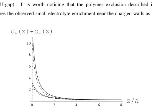
However, there is a concomitant migration of ions from the bulk to the gap due to the combined effects of electrostatic attraction by the charged walls coupled to a dielectric-mediated ionic flux from low (bulk) to high (gap) dielectric permittivity. Therefore, the equilibrium ion concentration inside the gap is given by (26b), provided the dielectric permittivity within the gap is replaced by that of the pure solvent. Accordingly, the modified Poisson-Boltzmann equation (26b) reduces to

(

)

* sinh * 2 2 2 2 ψ κ ς ψ ⋅ = ∂ ∂ a eff ( 30 )

where the effective Debye length has been properly renormalized to account for

salting-out effects: κeff2 ≡

              − ε ε ε ε κ2 exp 1 1 s s B .

3.2.2. Self-regulating surface charges

We have seen that, despite the greater effectiveness of multi-valent ions in screening the electrostatic potential and disfavouring the solvent-polymer compatibility,

28 they should have a modest role in polymer-assisted membrane fusion because of their smaller concentration at physiological conditions. The situation is reversed when we consider the membrane surface. Here the local concentration of cations such as calcium and magnesium is high and comparable to that of monovalent ions because divalent cations form tight complexes with the phosphate or carboxylic groups of lipid heads71,72,73,74_.

Regulation of the surface charges is described by introducing a few additional contributions to the surface energy:

Ion binding energy. Binding of a Z-valent ion to a charged membrane neutralizes

+

Z lipid heads. Letting

θ

_{to be the unknown fraction of neutralized sites (}0<

θ

<1_{), the}

surface concentration of a Z-valent ion is

θ

2

b Z

X

+ , where X is the fraction of charged

lipids and b the lipid surface area. Therefore, the binding energy reads: 2

dS EZ b Z X S + +

∫

− ₂

θ

, where

−

E

is the ion-lipid binding energy per single bond.

Entropy term. The entropy of mixing among occupied and vacant sites over the

membrane surface takes the standard form:

dS kT b Z X S )) 1 log( ) 1 ( log 2

∫

θ

θ

+ −

θ

−

θ

+ .

Surface electrostatics. Due to the partial neutralization of the charged lipids by tightly adsorbed ions, the membrane surface density is lowered from the initial value σ to σ(1−θ) (with _{/ b}2

eX

≡

σ _{). Thus, the electrostatic energy variation upon ion binding}

reads: z z dS S 0 ) ( ) 1 ( − ₌

∫

σ θ ψ .

Summing up, the energy terms a)-c), and introducing the polymer-surface interaction, we generalize equation ( 20 ) obtained for non-adsorbing membrane surfaces

= SUP E

[

0 2 2 2 (a /b )Xe(1− )⋅ (z)z= a S ψ θ _{( ) ( )}

_]

0 2 θ τ γ z _z +F + = ( 31 ) where:

[

log (1 )log(1 ) 2 2

θ

θ

θ

θ

+ − − +b Z XkTa

]

θ kT E Z+ −

. Calculating the chemical potential of an adsorbed ion by minimizing ( 31 ) with respect to

θ

, equating the surface

29 and bulk chemical potentials and introducing the dimensionless variables

kT e ( )/ * ψ ς ψ = _,

τ

*=

τ

(

ς

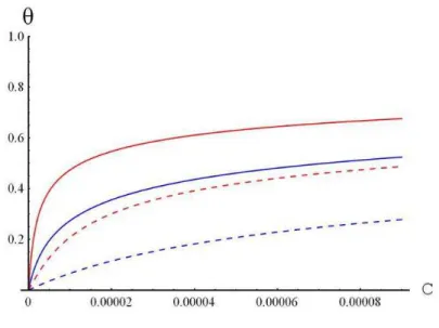
)/Φ1/2 _and ς = z/a_{, we get} ) ( 1 * θ θ θ eff zK c = − _{( 32 )}

From (32) we can obtain

θ

numerically. It is convenient to write the effective binding constant of a Z-valent ion as

≡ ) (θ eff K               − + + = + s o Z Z B K ε ε ψ*_ς 1 1 exp 2 0 ( 33 )

where Ko>1 is the intrinsic ion-membrane binding constant measured in pure

solvent at zero surface potential (Ko can be assimilated to the experimental ion binding

constant when the charged sites are dissolved into a sea of neutral lipids). The exponential term in (33) describes the electrostatic effect of the charged lipid headgroups on the ion binding. Unfortunately, no analytical expressions are available for the surface potential ψ * in mixed solvents. However, by numerically calculating

ψ

*ς=0 for different

values of the fraction of charged lipids concentration X, and interpolating the obtained curves with the expansion = = + + +

2 3 2 1 0 *

θ

θ

ψ

_ς A A A

…, we obtain the unknown coefficients A . This procedure transforms (32) into a Frumkin type equationj 75.

...)) ( exp( 1 2 3 2 1 * + + + = − + θ θ θ θ A A A Z K cz o ( 34 )

which is numerically solved for

θ

. Using these values for surface charge neutralization, we can use (26a,b) to calculate the polymer concentration and the electrostatic potential by replacing the fraction of charged lipids X by X(1−θ) _{in the} boundary condition (28b). Numerical results will be briefly described in section 5.

Although the bulk concentration of multivalent ions is much smaller than that of monovalent ones, their relative concentrations near the membrane surface are similar because of the stronger binding of multivalent cations.

30 3.2.3. Interaction between two charged surface in mixed electrolyte-polymer-solvent fluid.

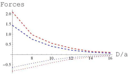
Once the electrolyte and polymer concentration profiles inside the gap have been calculated, we can derive the inter-membrane pressure. The total pressure P between two identical planar charged surfaces embedded in a multi-component fluid has been calculated by several authors. Andelman and co-workers obtained

i M i _i i M i _i n n h h n n P

∑

∑

= = ∂ ∂ − +       ∂ ∂       ∂ ∂ + = − 1 2 1 * 8 1 ς ψ ε ε π _{( 35 )}

for a mixture that contains M different species89 .ni is the concentration of each

component, h is the grand potential without any explicit ψ *-dependent electrostatic interactions (in our notation h=ψlim(z)→0H/S, with

H

given by (1B)). Here ni are polymer

concentration Φ(z)=τ2(z) and electrolyte concentrations c±(z). Using the analytical

expression for the dielectric permittivity given by (11), we find

[

1 2 3 4

]

2 P P P P a kT P= + + + − ( 36 )

(

)

2 1 ₈ 2( ) 1       ∂ ∂ Φ − + = z P s p s

ψ

ε

ε

ε

π

1 2 3 =Φ(1−N)+log(1−Φ)+

χ

Φ P P2 =−(c+ +c−) ) ( ) ( 2 4 Φ + + − Φ − =B c c P p s

ε

ε

ε

The first term, P , is the electrostatic pressure arising from the Maxwell stress 1

tensor, the second one, P , originates from the entropy of mixing of positive and 2

negative ions. This term is basically the Van’t Hoff osmotic pressure originating from a gas of charged particles. The third term, P3, describes the Van’t Hoff osmotic pressure of

a polymer solution. Finally, the last term, P4, describes an explicit coupling term

between electrolyte and polymer concentrations.

To find the net interaction between the plates, we subtract the reservoir pressure from the total pressure (36)

P P

P= −